Assessing Spatial and Temporal Distribution of Algal Blooms Using Gini Coefficient and Lorenz Asymmetry Coefficient

Algal bloom in an inland lake is characterized by significant spatial and temporal dynamics. Accurate assessment of algal bloom distribution and dynamics is highly required for tracing the causes of and creating countermeasures for algal bloom. Satellite remote sensing provides a fast and efficient way to capture algal bloom distribution at a large scale, but it is difficult to directly derive accurate and quantitative assessment based on satellite images. In this study, the Gini coefficient and Lorenz asymmetry coefficient were introduced to examine the spatio-temporal algal bloom distribution of Chaohu Lake, the fifth largest inland lake in China. A total of 61 remote sensing images from three satellite sensors, Landsat, Gaofen, and Sentinel were selected to obtain algal bloom distributions. By dividing remote sensing images into 0.01°*0.01° grid cells, the normalized difference vegetation index (NDVI) for each grid cell was derived, forming a spatial and time series database for quantitative analysis. Two coefficients, Gini coefficient and Lorenz asymmetry coefficient, were used to evaluate the overall intensity, unevenness, and attribution of algal bloom in Chaohu Lake from 2011 to 2020. The Gini coefficient results show a large variety of algal bloom in the spatial and temporal scales of Chaohu lake. The lake edge and northwestern part had longer lasting and more severe algal bloom than the lake center, which was mainly due to nutrient import, especially from three northwestern tributaries that flow through the upstream city. The Lorenz asymmetry coefficient revealed the exact source of the unevenness. Spatial uncertainties were mostly caused by the tiny areas with high NDVI values, accounting for 53 cases out of 61 cases. Temporal unevenness in northwestern and northeastern parts of the lake was due to the most severe breakout occurrences, while unevenness in the lake center was mainly due to the large number of light occurrences. Finally, the advantage of Gini coefficient and Lorenz asymmetry coefficient are discussed by comparison with traditional statistical coefficients. By incorporating the two coefficients, this paper provides a quantitative and comprehensive assessment method for the spatial and temporal distribution of algal bloom.

1 Introduction

Algal bloom in water areas has been a critical worldwide environment issue for the past several decades (Haag, 2007). Many studies have tracked long-term algal bloom outbreaks of various inland lakes in China (Wang et al., 2012; Yan et al., 2012; Huang et al., 2015; Zhang et al., 2015; Kang et al., 2016), U.S. (Hambright et al., 2010; Winston et al., 2014), India (Kamerosky et al., 2015), Mexico (Stumpf et al., 2003), and Canada (Hecker et al., 2012; Sorichetti et al., 2014). Since algal bloom is highly sensitive to various factors such as nutrients, temperature, wind speed, air pressure, and human controlling (Ahlgren, 1988; Vedernikov et al., 2007; Klemencic and Toman, 2010; Ribeiro et al., 2015; Wang et al., 2017), its spatial and temporal distribution is characterized as highly uneven and fluctuating, especially for inland lakes where the water flow and regeneration rate are lower. Therefore, an accurate description of spatial and temporal distribution is an important prerequisite for analyzing and controlling algal bloom outbreaks.

Satellite remote sensing has significant advantages for its large-scale and periodic observation, providing an efficient manner to observe large-scale algal blooms. Since the 1990s, the Landsat satellite has been used to monitor lake algal blooms and their dynamics (Galat and Sims, 1990; Richardson, 1996). Today there are several satellites that are widely used in algal bloom observation, i.e., the Landsat satellite (Ho et al., 2019), Sentinel satellite (Moita et al., 2016; Pirasteh et al., 2020), MODIS satellite (Lu and Tian, 2012; Zhang et al., 2015), Gaofen satellite (Hu et al., 2019), and GOCI satellite (Choi et al., 2014; Lou and Hu, 2014). Algal bloom indicators derived from satellite remote sensing bands include normalized difference vegetation index (NDVI) (Van Der Wal et al., 2010; Lin et al., 2016), FAI (Hu, 2009; Zhang et al., 2014; Page et al., 2018), Chla (Hu, 2009; Zhang et al., 2014; Page et al., 2018; Guan et al., 2020; Pompeo et al., 2021), etc. On this basis, various analyses are conducted on algal bloom distribution from spatio-temporal (Lu and Tian, 2012; Zhang et al., 2015; Page et al., 2018; Zabaleta et al., 2021) and vertical (Bosse et al., 2019) points of view. In 2019, a global spatio-temporal algal blooms analysis covering 71 large lakes from 33 countries based on Landsat five satellite images (Ho et al., 2019) revealed that algal bloom in over 2/3 of lakes had been increasing during the last 30 years. These studies show that the application of satellite remote sensing is a useful and efficient way to observe, track, and evaluate long-term and large-scale algal bloom distribution.

Although remote sensing images inversion can display the general coverage, severity, and evolution trend of algal bloom, the evaluation of distribution based on numerous images, especially for time series analysis, is subjective. Since algal bloom may grow and fade rapidly, its characteristics may be highly diverse in a couple of days (Lu and Tian, 2012; Zhang et al., 2020). Current research focuses less on the quantitative assessment method of algal bloom distributions. Using hotspots is one of the quantitative assessment methods that has been applied in spatial distribution analysis (Wei et al., 2021; Zabaleta et al., 2021). Generally, a quantitative description of temporal and spatial distribution of algal blooms is still lacking. Indices that accurately and briefly abstract the key information of algal bloom distribution features are highly needed. This requirement is more important when incorporating long-term temporal analysis in analysis.

In this paper, we focus on the assessment method of algal bloom distribution of Chaohu Lake from 2011 to 2020. Two indices, the Gini coefficient and Lorenz asymmetry coefficient, which are originally proposed to assess citizen income inequality, are applied to spatial and temporal distribution analysis of algal bloom. These two indices have been adopted to analyze river flow variability and biological species variability in previous studies (Damgaard and Weiner, 2000; Zhen-Xiang et al., 2004; Jawitz and Mitchell, 2011; Masaki et al., 2014; Zhang et al., 2020). It is considered suitable to use these two indices to measure and explain this variability. The Gini coefficient is used to measure the spatial or temporal distribution inequality (unevenness) of algal blooms, while the Lorenz asymmetry coefficient explains whether the unevenness is caused by a small number of large NDVI values or a large number of small NDVI values. To be specific, for spatial analysis, the two coefficients indicate the extent of lake-wide variability of algal bloom and which area contributes to the unevenness; for temporal analysis, the two coefficients indicate the temporal variability of algal bloom in each grid cell, and which occurrences contribute most to the unevenness.

The study site and data of Chaohu Lake are described in section 2. The application of the Gini coefficient and Lorenz asymmetry coefficient in assessing algal bloom spatial and temporal distribution are explained in section 3. Section 4 presents the result of spatial and temporal distribution with discussion. A conclusion is given in section 5.

2 Study Area and Data

2.1 Chaohu Lake

Chaohu Lake (31°25' ∼ 31°42′N, 117°17' ∼ 117°50′E), located in central-eastern China, is the fifth largest inland freshwater lake of China. The lake covers an area of 780 km², with a length of 55 km in longitude and a width of 21 km in latitude (Shang and Shang, 2005). A total of 90% of the Chaohu Lake is supplied by surface runoff (Yang et al., 2013), consisting of 10 major inflow-tributaries entering the lake. The location and distribution of Chaohu Lake is shown in Figure 1.

FIGURE 1

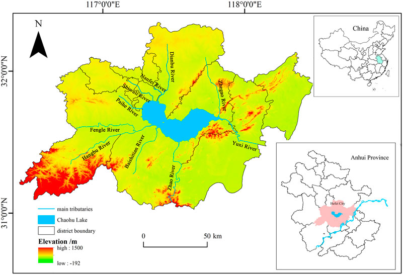
FIGURE 1. Location and distribution of Chaohu Lake.

Algal bloom of Chaohu Lake has occurred almost every summer in the past several decades (Shang and Shang, 2005). Since the 1970s, with rapid industry and population development, nutrients and organic matter such as nitrogen and phosphorus in the lake have rapidly increased, resulting in the frequent occurrence of algal bloom (Kong et al., 2013). Satellite remote sensing data showed that algal bloom in Chaohu Lake has broken out almost every year in the past 30 years, with an average annual outbreak frequency of six times (Damgaard and Weiner, 2000). In the early 1980s, the algal blooms were mainly distributed in the northwest and northeast lake areas. During 1983–1990, the algal bloom gradually moved to the lake center. In 1990, the algal bloom occurred throughout the lake. From 1999 to 2017, algal bloom began to shrink gradually, with most algal blooms concentrated in the northwest lake area (Li S M, 2019). The initial time of algal bloom outbreak in each year is gradually getting earlier, and the duration is gradually increasing (Damgaard and Weiner, 2000).

2.2 Data Sources

In this study, three types of satellite sensors, the Landsat 5/7/8 satellite, GF-1 satellite, and Sentinel-2 satellite are used to obtain the algal distribution of Chaohu Lake. Table 1 lists the main parameters of the three sensors. All candidate images from May to October between the years 2011–2020 were examined, and only cloud-free images with algal bloom areas greater than 50 km² were considered. A total of 61 remote sensing images were obtained with significant algal bloom coverage and almost no cloud coverage. Table 2 shows the date and source of selected images. The number of images varies widely from year to year due to the different severity of algal bloom and image quality.

TABLE 1

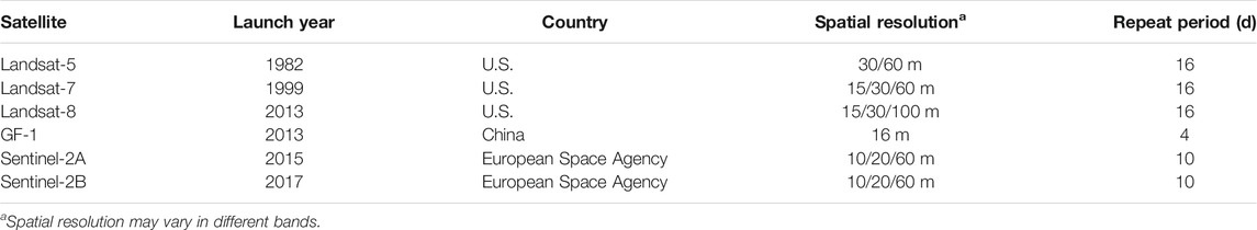
TABLE 1. Parameters of Landsat satellite, GF-1 satellite, and Sentinel satellite.

TABLE 2

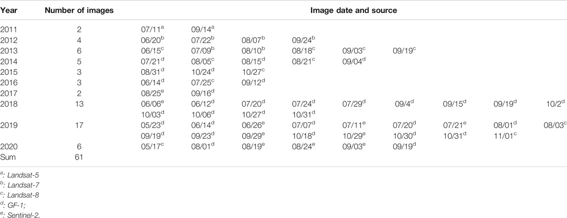
TABLE 2. Satellite images dates and sources .

All the images were checked or preprocessed to make sure atmospheric correction was applied. The aim of atmospheric correction is to eliminate the influence of atmospheric and illumination factors on the reflection of ground objects. In this study, the Landsat-5, Landsat-7, and Landsat-8 data were L2 grade and corrected by the Landsat official production system including radiometric and geometric correction (https://www.usgs.gov/faqs/does-landsat-level-1-data-processing-include-atmospheric-correction). The Sentinel-2 data (L2A level) used in this paper were generated from 1C products based on scenario classification and atmospheric correction algorithms. (https://sentinels.copernicus.eu/web/sentinel/technical-guides/sentinel-2-msi/level-2a-processing). The GF-1 data were pre-processed using FLAASH mode in ENVI 15.3 software.

2.3 NDVI Indicator

Since green algae has similar spectral characteristics with terrestrial vegetation, some indicators that reflect vegetation are widely adopted to characterize algal bloom coverage of a water area, such as FAI and NDVI (Zhu et al., 2020). In this study, due to the lack of short-wave infrared band data in the GF-1 sensor, the NDVI index was adopted as an indicator of algal bloom. The derivation of NDVI is:

$NDVI=\frac{NIR-R}{NIR+R}(1)$

where NIR is the reflectance of the near-infrared band and R is the reflectance of the red band. The NDVI value ranges from -1 to 1. Positive NDVI denotes the existence of algal bloom, and higher NDVI indicates higher algal bloom severity. Bands of NIR and R for each satellite used in this study are listed in Table 3.

TABLE 3

TABLE 3. NIR and R bands for Landsat-5, Landsat-7, Landsat-8, GF-1, and Sentinel-2 satellites.

3 Materials and Methods

3.1 Extraction of Lake Cells

Although the distribution of algal bloom can be roughly seen and analyzed from the NDVI distribution map of remote sensing inversion, it is still very important to divide the lake area into grid cells for quantitative assessment, because appropriate cell division can facilitate further calculation and make the spatial and temporal evaluation results closer to the real value. Grid cell division has been used in various spatial analyses for quantitative analysis. Masaki et al. (2014) extracted major river channel cells to analyze the variability of inflow regimes for different parts of rivers; Guevara-Escobar et al. (2007) used grid-divided data to evaluate rainfall distribution patterns; Raziei and Pereira (2013) and Das et al. (2014) interpolated and gridded rainfall distributions to 0.5°*0.5° and 1°*1° grid cells respectively for spatial analysis. With this consideration, the Chaohu Lake area was divided into equidistant grids for quantitative spatial and temporal analysis. First, the shape of Chaohu Lake was clipped using DEM contours. To avoid the confusion of lake edge caused by water level fluctuation, the DEM contour latitude was set slightly lower than the normal water level. The clipped lake area was then taken as the “uniform lake shape” for all images, assuring the location of grids was consistent in every image. Second, the lake area was divided by horizonal and vertical parallel lines with 0.01° distance, generating 850 0.01°*0.01° grid cells. In this way, the distribution of algal bloom was represented by uniform grid data of mean NDVI. The grid data were regarded as the regularized vector for quantitative spatial and temporal analysis. Figure 2 shows an example of the NDVI distribution from 2014.08.15 with grid cell division.

FIGURE 2

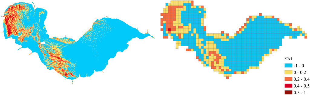
FIGURE 2. NDVI distribution with grid cell division from 2014.08.15.

Based on grid cell division, spatial and temporal distribution can be analyzed quantitatively and comprehensively. Figure 3 shows an illustration of the spatial and temporal analysis based on grid cells. Spatial analysis is based on grid cells of each image, while temporal analysis is derived by the NDVI time series of each grid cell from different images.

FIGURE 3

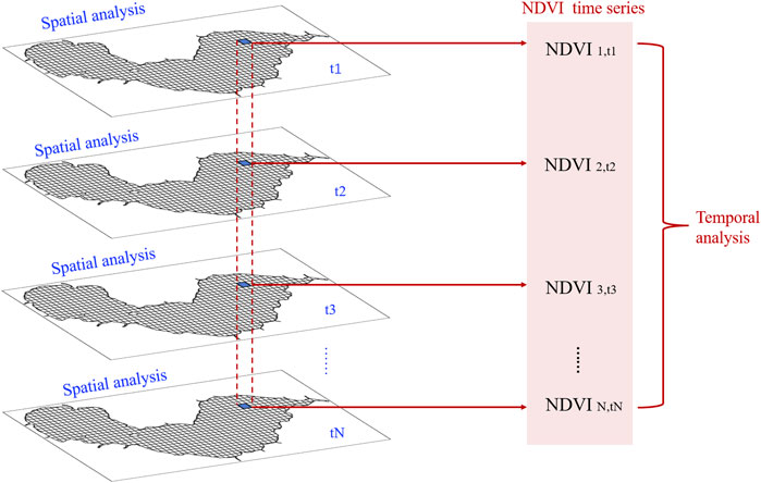
FIGURE 3. Illustration of spatial and temporal analysis based on grid cells.

3.2 Gini Coefficient and Lorenz Asymmetry Coefficient

In this paper, the Gini coefficient and Lorenz asymmetry coefficient are adopted to evaluate the shape of NDVI-area curve. The advantage of such coefficients is that they can describe not only the variability of NDVI over different areas but also the attribution of variability. As mentioned above, the algal bloom distribution, which is represented by NDVI, varies largely in different areas and different years in Chaohu Lake. The two indices help the interpretation of spatial and temporal inequality of algal bloom. The Gini coefficient provides the total inequality degree, while the Lorenz asymmetry coefficient interprets whether the inequality is caused by high-NDVI elements or low-NDVI elements. Considering these features of indices, we attempted to give a comprehensive description and attribution of algae distribution inequality.

3.2.1 Gini Coefficient

The Gini coefficient was first introduced by Corrado Gini in 1912 (Gini, 1912) to quantify inequality of household incomes. In the past decades, the Gini coefficient has been extended to environment sciences, such as inequality of plant species distribution (Ma et al., 2006; Shi et al., 2012), precipitation inequality (Shi et al., 2012), and river flow temporal distribution (Masaki et al., 2014), etc. Hereafter, we apply the Gini coefficient to spatial and temporal distribution inequality of Chaohu Lake.

The Gini coefficient G is given by (Eytan, 1972; Kimura, 1994)

$G=\frac{{{\displaystyle \sum }}_{i=1}^n{{\displaystyle \sum }}_{j=1}^n|y_i-y_j|}{2n^2\overline{y}}(2)$

where n is the number of individuals, $y_i$ is the income of individual i, and $\overline{y}$ is average income of all individuals. Note that $y_1$ ≤ $y_2$ ≤…≤ $y_n$. A higher Gini coefficient reflects a higher income diversity, and vice versa. When applying the Gini coefficient to assess the unevenness of algal bloom, n represents the number of total grids, $y_i$ denotes algal bloom amount which is represented by NDVI in grid i.

The Gini coefficient is more widely interpreted using a graphical manner, known as the Lorenz curve. The Lorenz curve is obtained by aggregating the percentage of individuals (horizonal axis) and the percentage of incomes (vertical axis). In this study, the horizonal and vertical axes of the Lorenz curve are the cumulative percentage of the grid area and the cumulative percentage of algal blooms, as shown in Figure 4. The graphical interpretation of the Gini coefficient is the ratio of area A to the triangle (A + B) in Figure 4. Note that (A + B) = $\frac{1}{2}$, and the relationship between G and A is:

$G=\frac{A}{A+B}=2A(3)$

FIGURE 4

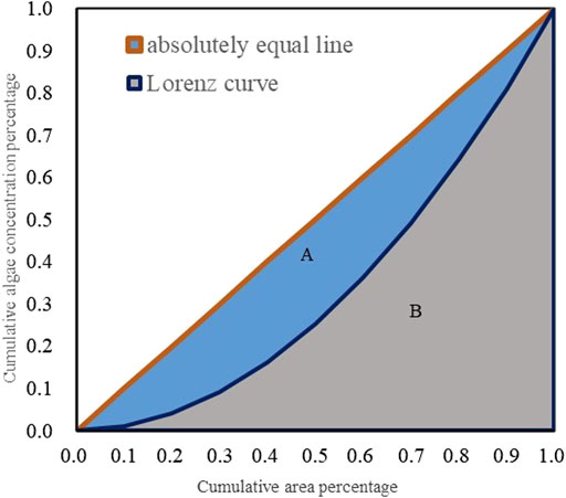
FIGURE 4. Sketch of the Lorenz curve and Gini coefficient.

The slope of the Lorenz curve reveals the inequality degree of algal bloom spatial distribution. Imagining a perfectly even distribution of algal bloom where a 1% increase in area corresponds to a 1% increase in algal cumulation, the Lorenz curve is a line with slope 1 (y = x), which is called the “absolutely equal line”. For unevenly distributed algal bloom area distribution, the Lorenz curve is under the absolutely equal line. The farther the Lorenz curve is from the y = x line, the more uneven the algal bloom distribution is, and the higher the G value is.

3.2.2 Lorenz Asymmetry Coefficient

Although the Gini coefficient presents an efficient indicator to describe the unevenness of algae distribution, it also has some limitations. Since G = 2A, it is possible that different Lorenz curves may have the same Gini coefficient. Figure 5 shows NDVI distributions from 2016.06.14 to 2018.09.19. Both Gini coefficients are 0.12, however their algal bloom intensity and distribution are quite diverse, also the shape of the Lorenz curves is different. This indicates that the Gini coefficient is insufficient to describe algal bloom distribution, and the Lorenz asymmetry coefficient is then adopted.

FIGURE 5

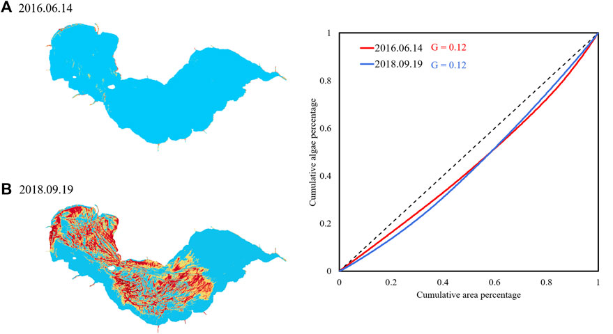
FIGURE 5. Example of images with the same G but different algal bloom distribution and Lorenz curve.

The Lorenz asymmetry coefficient, denoted as S, is given by (Damgaard and Weiner, 2000):

$S=F+L(4)$

$\delta =\frac{\overline{x}-x_m}{x_{m+1}-x_m}(5)$

$F=\frac{m+\delta }{n}(6)$

$L=\frac{{{\displaystyle \sum }}_{i=1}^m{x}_i+\delta x_{m+1}}{{{\displaystyle \sum }}_{i=1}^n{x}_i}(7)$

where m is the number of pixels with a value less than $\overline{x}$. In this paper, x denotes NDVI series for each grid. The graphical explanation to F and L is the x-coordinate and the y-coordinate of the point with slope one of the Lorenz curve. If S = 1, the coordinate (F, L) lies exactly on line x + y = 1. If S > 1, the coordinate (F, L) lies above line x + y = 1; if S < 1, the coordinate (F, L) lies below line x + y = 1. Figure 6 shows three types of Lorenz curve with S < 1, S = 1, and S > 1. Triangular marks denote points with slope = 1. Note that S=F + L for the three curves in Figure 6: 0.59 = 0.47 + 0.12, 1 = 0.56 + 0.44, 1.11 = 0.65 + 0.46.

FIGURE 6

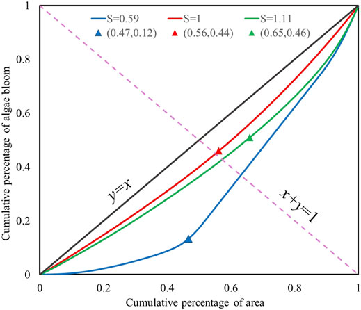
FIGURE 6. Examples of Lorenz curves with different S values. Blue, red, and green colors indicate results for algal bloom distribution on 08/01/2020, 09/04/2014, and 10/31/2018, respectively.

The significance of the Lorenz asymmetry coefficient S is that when S > 1, the inequality of algal bloom distribution is mostly due to the small amount of high NDVI values, which is also shown in the upper-right tail of the Lorenz curve; when S < 1, the inequality of algal bloom distribution is mostly due to large amounts of low NDVI values, which is shown in the lower-left tail of the Lorenz curve; S = 1 denotes that both parts have the same contribution to algal bloom inequality. Therefore, we can infer from Figure 6 that algal bloom unevenness on 2018.10.31 was mostly due to large NDVI elements, and unevenness on 2020.08.01 was mostly due to small NDVI elements. This provides clear notice about areas with great diversity, and, if the diversity is due to large elements (S > 1), it is an explicit warning of algal concentration.

4 Results and Discussion

4.1 Spatial Distribution of NDVI in Chaohu Lake

4.1.1 General Spatial Distribution Based on Mean NDVI

The 61 remote sensing images listed in Table 1 were processed to obtain the NDVI distribution in grid cells. Figure 7 shows the monthly maximum NDVI from May to October. It can be clearly indicated that the algal bloom develops from May, reaching its peak in September, and then slightly decreases in October. This trend is highly accordant with the temperature trend of the Chaohu Lake area. The algal bloom first concentrates at the northwestern part of the lake (June), and then spreads to the lake center (July and August) and the whole lake (September). Besides, the lake edge and tributaries have relatively higher NDVI values than the lake center, even in May when there is almost no algal bloom throughout the lake. This indicates that algal bloom of Chaohu Lake originates from the lakeside, and is mainly imported from lake tributaries. The upper reaches of the three northwestern tributaries, Nanfei river, Paihe river, and Shiwuli river (Figure 1), flowing through Hefei City, which is the capital city of Anhui province with a population over 5.7 million, brings massive nutrients that trigger algal bloom at the northwestern lake area. This inference is also proved in relative studies. It is concluded that nutrient and climate conditions are two dominant issues for algal blooms of Chaohu Lake (Li et al., 2019), while Chen and Liu (2014) stated that tributaries bring 68.5% and 76.5% of nutrients (TN and TP) into Chaohu Lake; three northwestern rivers: Nanfei river, Paihe river, and Shiwuli river have the highest comprehensive pollution index among all tributaries.

FIGURE 7

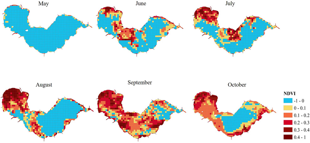
FIGURE 7. Monthly maximum NDVI distribution of Chaohu Lake, 2011-2020.

4.1.2 Gini Coefficient and Lorenz Asymmetry Coefficient

1) Gini coefficient and Lorenz asymmetry coefficient results

The Gini coefficients (G) and Lorenz asymmetry coefficients (S) of 61 images are shown in Figure 8. G varies from 0.04 to 0.2, indicating a diverse unevenness of algal bloom. There are 53 cases with S > 1, accounting for 87% of the total 61 cases. Recalling that S implies the source of unevenness, this reveals that the algal bloom unevenness of Chaohu Lake is mostly due to the small amount of high NDVI value areas, in other word, the tiny severe algal-concentrated areas.

2) Comprehensive discussion using mean NDVI and G

FIGURE 8

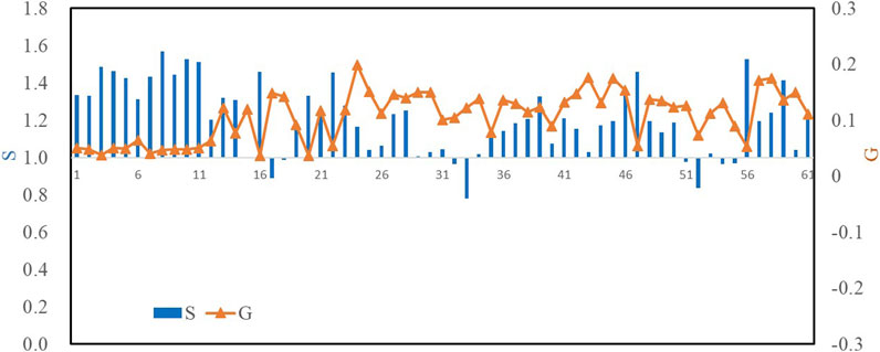
FIGURE 8. Gini coefficients and Lorenz asymmetry coefficients from 2011 to 2020.

By coupling mean NDVI and G, we can categorize the spatial distribution of algal bloom into four types: heavy and uneven type, heavy and even type, light and uneven type, and light and even type. Figure 9 shows the four types with representative examples for each type. The heavy and even type and light and uneven type are in the majority, accounting for 53 cases among all 61 cases. In addition, it can be clearly found that G can be diverse in different cases even if they have the same mean NDVI, and mean NDVI can be diverse in different cases even if they have the same G. This demonstrates that univariate assessment is insufficient to describe the distribution of algal bloom. These four types of algal bloom distribution characterized by mean NDVI and G are helpful in identifying the distribution patterns of algal bloom and taking targeted measures.

3) Comprehensive discussion using mean NDVI, G, and S

FIGURE 9

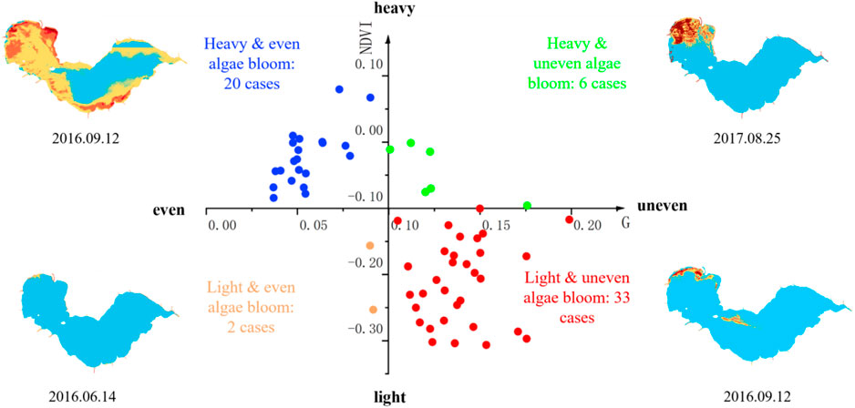
FIGURE 9. Four types of algal bloom characterized by mean NDVI and G with example images.

In order to analyze the integrated assessment of mean NDVI, G, and S, four distribution maps are chosen from 61 images as examples: 1. minimum G (2014.08.21); 2. maximum G (2017.08.25); 3. minimum mean NDVI value (2019.05.23); and 4. maximum mean NDVI value (2019.10.29). Their NDVI distributions, Lorenz curves, mean NDVI, G, and S are shown in Figure 10.

FIGURE 10

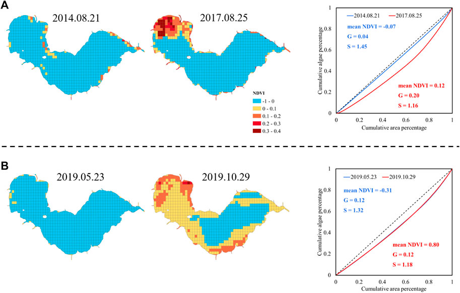
FIGURE 10. Examples of algae distribution with (A) maximum and minimum G, and (B) maximum and minimum mean NDVI.

The lowest and highest G (Figure 10A) occurred on 2014.08.21 and 2017.08.25, respectively. The NDVI map from 2014.08.21 has only sporadic high NDVI cells, emerging with an even algae distribution. In contrast, NDVI on 2017.08.25 is quite diverse as the northwestern part of the lake and lake side had significantly high NDVI, while NDVI in the lake center kept at a low level. This diversity is the reason for the high G value.

The minimum and maximum mean NDVI, (Figure 10B) which is −0.31 and 0.80, occurred on 2019.05.23 and 2019.10.29, respectively. Note that the NDVI value ranges within [−1,1], thus an average of 0.80 in NDVI indicates severe algal bloom. Algae coverage on 2019.10.29 reached 69%, while on 2019.05.23 was only 10%. However, it is interesting that their Gini coefficients are indeed the same although the NDVI difference is huge, because the Gini coefficient is related to the percentage quantiles but not the NDVI value itself.

Lorenz asymmetry coefficients (S) of the four cases are greater than 1, revealing that the unevenness of the algal bloom distribution of four cases is mainly due to the small amount of large NDVI grid cells. S value on 2014.08.21 was the greatest among the four images, revealing that the very small areas with highest NDVI in the map, are the reason for unevenness. In conclusion, mean NDVI, G, and S form a comprehensive description indicator system describing the severity and spatial distribution of algal bloom, thus providing an alternative way to quantitatively assess multiple remote sensing images.

4.2 Temporal Analysis of Algal Bloom

4.2.1 General Temporal Distribution Based on Frequency Analysis

By deriving the NDVI time series data of each grid cell, temporal analysis is carried out to reveal the change trend of algal bloom distribution for each grid cell. Here, the occurrence frequency map that consists of the frequency of each grid is derived. The frequency of grid i, $F_i$, is denoted by:

$F_i=\frac{T_i}{T}(8)$

where $T_i$ represents counts of images with $\overline{NDVI}$ >0 for grid i; $T$ represents the number of total images, which is 61 in this study. $\overline{NDVI}$ >0 is regarded as the indication of algal bloom occurrence. The frequency map is calculated and drawn, as shown in Figure 11.

FIGURE 11

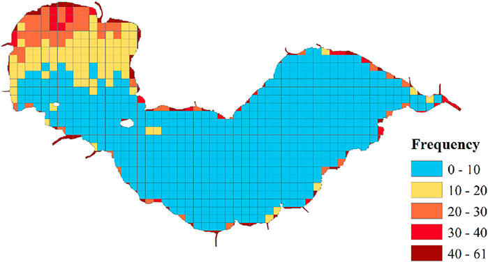
FIGURE 11. Algal bloom frequency map for each grid cell (number of grid cells: 850).

It is clearly indicated from Figure 11 that the northwestern part of the lake and lake edge have significantly high frequency in algal bloom. In addition, almost all tributary estuaries (tiny branches at the lake sides) have a much higher frequency than the lake center. Similar conclusions are inferred in Zhang et al. (2015) and Liu et al. (2017) where the northwestern part of the lake has the highest frequency of algal bloom during 2000–2013, and the primary source of algal bloom is tributary and lakeshore imports.

In the northwestern part of the lake, algal bloom frequency gradually decreases from the lake side to the lake center. By reviewing NDVI distribution images, the reason is the occasional spread of algal bloom from the lake side to the lake center. Severe algal bloom may spread from the northwestern lake edge to the lake center, and the nearby northwestern lake area suffers.

4.2.2 Gini Coefficient and Lorenz Asymmetry Coefficient

1) Gini coefficient and Lorenz asymmetry coefficient results

The Gini coefficients and Lorenz asymmetry coefficients for each grid are shown in Figure 12A indicates that the Gini coefficient varies from 0.03 to 0.15 throughout the lake. In contrast with results of mean NDVI and frequency, the lake edge, where both frequency and mean NDVI are high, has the lowest G. This is because the lake edge area has a “stable and high” NDVI value during 2011–2020, and a stable NDVI level means low variance and low G. In contrast, the lake center has a relatively mixed G value, which is due to a high variance of NDVI values caused by occasional algal bloom occurrences.

FIGURE 12

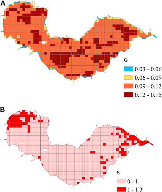
FIGURE 12. Map of (A) Gini coefficient and (B) Lorenz asymmetry coefficient for each grid cell.

Lorenz asymmetry coefficient S is divided and presented into two categories: S > 1 and S < 1, shown in Figure 12B. It can be clearly observed from Figure 12B that grid cells with S > 1 concentrate in the northwestern and northeastern areas, with a total of 124 grid cells. It means that the unevenness of these areas is due to the most severe occurrences among the 61 occurrences. In other words, these areas had a few extraordinarily severe algal bloom events, and these events caused the distribution unevenness in the temporal dimension.

2) Discussion on the sources of unevenness with S > 1.

Areas with S > 1 are more concerning in this study, as they imply the unevenness is due to high NDVI value occurrence which indicates severe algal bloom occurrences. Therefore, for the 124 grid cells with S > 1, the occurrences that contribute most to the unevenness of each grid cells are singled out. If one occurrence is responsible for multiple grid cells, the frequency is recorded by counts. We found that 39 occurrences were responsible for the unevenness of S > 1, as shown in Figure 13. Let us only take the occurrences with highest count for example, where the occurrence on 2019.10.29 involved 82 counts of all 124 grid cells. It implies that the algal bloom event on 2019.10.29 was a significant outlier that was responsible for the temporal unevenness of 2/3 grid cells. It is not surprising because the occurrence on 2019.10.29 was also mentioned in Figure 10B as the highest mean NDVI during 2011–2020. Also, this event was reported by the Department of Ecology and Environment of Anhui Province, and described as a “partial bloom”, which is much rarer and more serious than “sporadic bloom” that often occurs (Department of Ecology and Environment of Anhui Province).

FIGURE 13

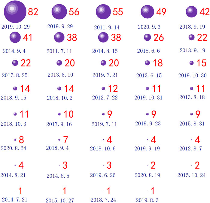
FIGURE 13. Counts of dates that contribute to unevenness of grid cells with S > 1.

It can be inferred from the above analysis that the Gini coefficient combined with the Lorenz asymmetry coefficient is able to quantify algal bloom distribution spatially and temporally and examine the origination of unevenness by “overlapping” numerous algal bloom events. Therefore, it provides a quantitative and useful guideline for researchers and operators to rank or evaluate numerous algal bloom occurrences over time, and track influence factors for algal blooms in specific lake areas.

4.3 Comparison of the Gini Coefficient and Lorenz Curve With Other Statistical Coefficients

Since the Gini coefficient and Lorenz curve are descriptions of unevenness of distribution, there are some existing coefficients that also describe the degree of data variations, such as variance and standard deviation. As analyzed in Masaki et al. (2014) and Milanovic (1997), the Gini coefficient is proportional to the coefficient of variation and standard deviation. Also, the Lorenz curve has similarities with cumulative distribution curve (CDF) in statistics, but they have not been compared as far as we know. Hereby, the relationship and distinction between these variables are explored using the dataset in this study.

4.3.1 Comparison Between Gini Coefficient With Other Statistical Coefficients

Fitting performance between G ∼ variance and G ∼ standard deviation based on spatial and temporal results are derived and shown in Figure 14 and Figure 15, respectively. The results show that the Gini coefficients in this study also have fine relationships with variance and standard deviation. The regression function type is the same as the results from Masaki et al. (2014), that is, a linear relationship between G and standard deviation, and polynomial relationship between G and variance. Nevertheless, the coefficient G has an outstanding feature over the other two coefficients: the G value is normalized to [0,1] regardless of the value of samples data, which allows it to be used as a universal indicator for all cases.

FIGURE 14

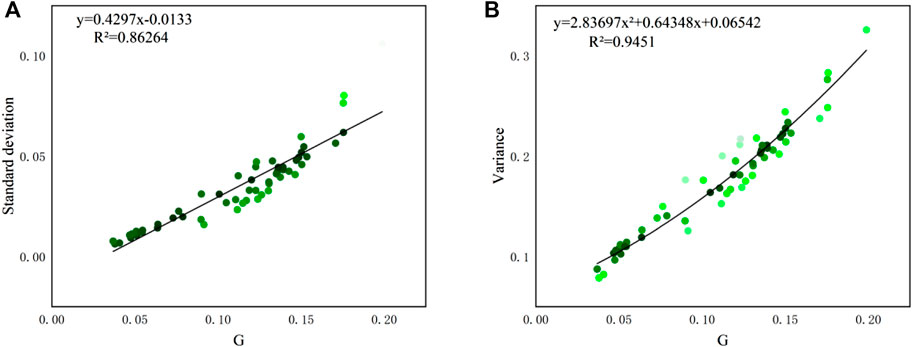
FIGURE 14. Relationships between (A). G ∼ variance and (B). G ∼ standard deviation of spatial distribution (sample size: 61).

FIGURE 15

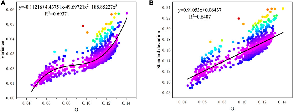
FIGURE 15. Relationships between (A). G ∼ variance and (B). G ∼ standard deviation of temporal distribution (sample size: 850).

4.3.2 Comparison Between Lorenz Curve With CDF Curve

The CDF curve, which is derived by aggregating the NDVI value in ascending order and its corresponding non-exceedance probability, can also ascertain the variability of samples in the form of curves. Here, the four NDVI distributions in Figure 10 are taken as a study example to compare the performances of CDF and Lorenz curves. Figure 16 shows the results of CDF and Lorenz curves for each distribution.

FIGURE 16

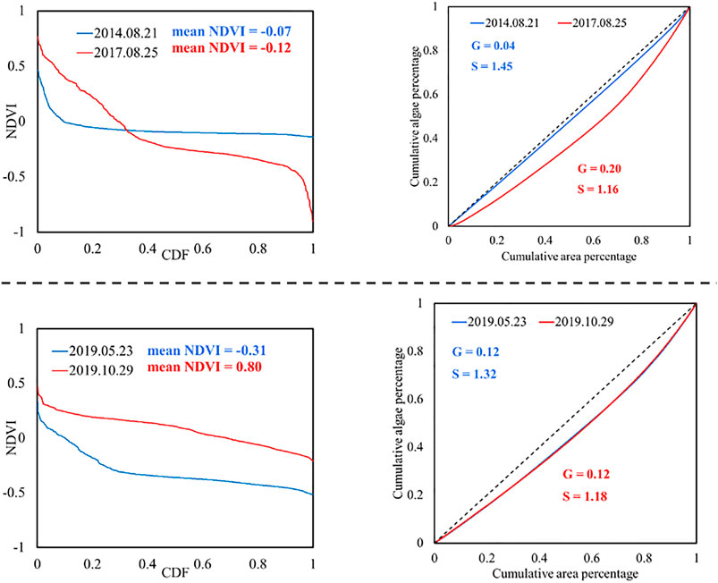
FIGURE 16. Comparison between CDF curve and Lorenz curve.

Figure 16 shows that both the CDF curve and Lorenz curve can reveal the variability features of spatial distributions. However, the CDF curve has similar limitations with variance and standard deviation in that it is not a universal coefficient, for its vertical axis (NDVI) varies with the NDVI values. The Lorenz curve, however, has an axis of cumulative percentage that is restricted within [0, 1]. Besides, the features of the Lorenz curve can be interpreted by the Gini coefficient and Lorenz asymmetry coefficient. By these two coefficients we can easily judge various distributions without comparing the curves. However, it is not convenient to compare various CDF curves as there is no such scalar coefficient to describe curve features. Although the CDF curves in Figure 16 are very diverse and it is easy to tell the difference, it could be confusing in comparing various sample sets with similar distributions. In conclusion, the Lorenz curve outperforms the CDF curve in assessment analysis for its regularization and comparability.

5 Conclusion

This paper examined the characteristics of algal bloom distribution between 2011 and 2020 using mean NDVI, Gini coefficient, and Lorenz asymmetry coefficient of Chaohu lake, China. By dividing 61 remote sensing images into equidistant grid cells, statistical analysis can be carried out based on grid cell data to explore spatial and temporal distribution and trend in a quantitative way. Results suggest that algal bloom is severe at the lake edge and northwestern part of Chaohu Lake owing to tributary and lakeside nutrient imports. Lorenz asymmetry coefficient is applied to detect the source of unevenness, and the primary source of spatial distribution unevenness is the small area with very high NDVI values. Temporal analysis shows that the northwestern part and lake edge has very high algal bloom frequency but low Gini coefficient, indicating a stable and severe algal bloom situation. Lorenz asymmetry coefficient reveals that unevenness in the 124 grid cells concentrated in the northwestern and eastern parts of the lake is due to the most severe algal bloom occurrences.

Analysis in this paper indicates that mean NDVI, Gini coefficient, and Lorenz asymmetry coefficient can comprehensively and quantitively describe the distribution characteristics of lake algal bloom, while any single coefficient is one-sided and insufficient to accurately depict the distribution information. The algal bloom distribution may be different even if they have the same mean NDVI or Gini coefficient. The compound assessment method could allow researchers to identify algal bloom distribution patterns as well as sources to the unevenness. Possible extensions of this work will include the analysis of connections between algal booms and meteorological factors for the selected extreme occurrences, and the application of the methodology to assessment in other spatial distributions.

Data Availability Statement

The original contributions presented in the study are included in the article/supplementary material, further inquiries can be directed to the corresponding author.

Author Contributions

TZ wrote the paper and analyzed the results. CN and MZ calculated the Gini coefficients and Lorenz asymmetry coefficients, and concluded literature review for this paper. PX designed the research idea and layout of paper.

Funding

This research was funded by the National Science and Technology Major Project of China (grant no. 2017ZX07603-002) and the Natural Science Fund of Anhui Province (grant nos. 2008085ME158 and 2008085ME159).

Conflict of Interest

The authors declare that the research was conducted in the absence of any commercial or financial relationships that could be construed as a potential conflict of interest.

Publisher’s Note

All claims expressed in this article are solely those of the authors and do not necessarily represent those of their affiliated organizations, or those of the publisher, the editors and the reviewers. Any product that may be evaluated in this article, or claim that may be made by its manufacturer, is not guaranteed or endorsed by the publisher.

References

Ahlgren, G. (1988). Phosphorus as Growth-Regulating Factor Relative to Other Environmental Factors in Cultured Algae. Hydrobiologia 170, 191–210. doi:10.1007/bf00024905

CrossRef Full Text | Google Scholar

Bosse, K. R., Sayers, M. J., Shuchman, R. A., Fahnenstiel, G. L., Ruberg, S. A., Fanslow, D. L., et al. (2019). Spatial-temporal Variability of In Situ Cyanobacteria Vertical Structure in Western Lake Erie: Implications for Remote Sensing Observations. J. Great Lakes Res. 45, 480–489. doi:10.1016/j.jglr.2019.02.003

CrossRef Full Text | Google Scholar

Chen, Y.-Y., and Liu, Q.-Q. (2014). On the Horizontal Distribution of Algal-Bloom in Chaohu Lake and its Formation Process. Acta Mech. Sin. 30, 656–666. doi:10.1007/s10409-014-0078-x

CrossRef Full Text | Google Scholar

Choi, J.-K., Min, J.-E., Noh, J. H., Han, T.-H., Yoon, S., Park, Y. J., et al. (2014). Harmful Algal Bloom (HAB) in the East Sea Identified by the Geostationary Ocean Color Imager (GOCI). Harmful Algae 39, 295–302. doi:10.1016/j.hal.2014.08.010

CrossRef Full Text | Google Scholar

Damgaard, C., and Weiner, J. (2000). Describing Inequality in Plant Size or Fecundity. Ecology 81, 1139–1142. doi:10.1890/0012-9658(2000)081[1139:diipso]2.0.co;2

CrossRef Full Text | Google Scholar

Das, P. K., Chakraborty, A., and Seshasai, M. V. R. (2014). Spatial Analysis of Temporal Trend of Rainfall and Rainy Days during the Indian Summer Monsoon Season Using Daily Gridded (0.5° × 0.5°) Rainfall Data for the Period of 1971-2005. Met. Apps 21, 481–493. doi:10.1002/met.1361

CrossRef Full Text | Google Scholar

Department of Ecology and Environment of Anhui Province (2019). Monitoring results of emergency prevention and control of cyanobacteria in Chaohu Lake from October 28 to November 3, 2019. Available at: https://sthjt.ah.gov.cn/public/21691/110831651.html (Accessed November 13, 2019) (In Chinese).

Eytan, S. (1972). Relation between a Social Welfare Function and the Gini index of Income Inequality. J. Econ. Theor. 4, 98–100. doi:10.1016/0022-0531(72)90167-6

CrossRef Full Text | Google Scholar

Galat, D. L., Verdin, J. P., and Sims, L. L. (1990). Large-scale Patterns of Nodularia Spumigena Blooms in Pyramid Lake, Nevada, Determined from Landsat Imagery: 1972?1986. Hydrobiologia 197, 147–164. doi:10.1007/bf00026947

CrossRef Full Text | Google Scholar

Gini, C. (1912). Variabilità e mutabilità. Contributo allo Studio delle Distribuzioni e delle Relazioni Statistiche. Bologna: C. Cuppini

Google Scholar

Guan, Q., Feng, L., Hou, X. J., Schurgers, G., Zheng, Y., and Tang, J. (2020). Eutrophication Changes in Fifty Large Lakes on the Yangtze Plain of China Derived from MERIS and OLCI Observations. Remote Sens. Environ. 246, 111890. doi:10.1016/j.rse.2020.111890

CrossRef Full Text | Google Scholar

Guevara-Escobar, A., González-Sosa, E., Véliz-Chávez, C., Ventura-Ramos, E., and Ramos-Salinas, M. (2007). Rainfall Interception and Distribution Patterns of Gross Precipitation Around an Isolated Ficus Benjamina Tree in an Urban Area. J. Hydrol. 333, 532–541. doi:10.1016/j.jhydrol.2006.09.017

CrossRef Full Text | Google Scholar

Haag, A. L. (2007). Algal Bloom Again. Nature 447, 520–521. doi:10.1038/447520a

PubMed Abstract | CrossRef Full Text | Google Scholar

Hambright, K. D., Zamor, R. M., Easton, J. D., Glenn, K. L., Remmel, E. J., and Easton, A. C. (2010). Temporal and Spatial Variability of an Invasive Toxigenic Protist in a North American Subtropical Reservoir. Harmful Algae 9, 568–577. doi:10.1016/j.hal.2010.04.006

CrossRef Full Text | Google Scholar

Hecker, M., Khim, J. S., Giesy, J. P., Li, S.-Q., and Ryu, J.-H. (2012). Seasonal Dynamics of Nutrient Loading and Chlorophyll A in a Northern Prairies Reservoir, Saskatchewan, Canada. J. Water Resource Prot. 04, 180–202. doi:10.4236/jwarp.2012.44021

CrossRef Full Text | Google Scholar

Ho, J. C., Michalak, A. M., and Pahlevan, N. (2019). Widespread Global Increase in Intense lake Phytoplankton Blooms since the 1980s. Nature 574, 667–670. doi:10.1038/s41586-019-1648-7

PubMed Abstract | CrossRef Full Text | Google Scholar

Hu, L., Zeng, K., Hu, C., and He, M.-X. (2019). On the Remote Estimation of Ulva Prolifera Areal Coverage and Biomass. Remote Sensing Environ. 223, 194–207. doi:10.1016/j.rse.2019.01.014

CrossRef Full Text | Google Scholar

Hu, C. (2009). A Novel Ocean Color index to Detect Floating Algae in the Global Oceans. Remote Sensing Environ. 113, 2118–2129. doi:10.1016/j.rse.2009.05.012

CrossRef Full Text | Google Scholar

Huang, C., Shi, K., Yang, H., Li, Y., Zhu, A.-x., Sun, D., et al. (2015). Satellite Observation of Hourly Dynamic Characteristics of Algae with Geostationary Ocean Color Imager (GOCI) Data in Lake Taihu. Remote Sensing Environ. 159, 278–287. doi:10.1016/j.rse.2014.12.016

CrossRef Full Text | Google Scholar

Jawitz, J. W., and Mitchell, J. (2011). Temporal Inequality in Catchment Discharge and Solute export. Water Resour. Res. 47, W00J14. doi:10.1029/2010wr010197

CrossRef Full Text | Google Scholar

Kamerosky, A., Cho, H., and Morris, L. (2015). Monitoring of the 2011 Super Algal Bloom in Indian River Lagoon, FL, USA, Using MERIS. Remote Sensing 7, 1441–1460. doi:10.3390/rs70201441

CrossRef Full Text | Google Scholar

Kang, L., He, Q.-S., He, W., Kong, X.-Z., Liu, W.-X., Wu, W.-J., et al. (2016). Current Status and Historical Variations of DDT-Related Contaminants in the Sediments of Lake Chaohu in China and Their Influencing Factors. Environ. Pollut. 219, 883–896. doi:10.1016/j.envpol.2016.08.072

PubMed Abstract | CrossRef Full Text | Google Scholar

Kimura, K. (1994). A Micro-macro Linkage in the Measurement of Inequality: Another Look at the Gini Coefficient. Qual. Quant. 28, 83–97. doi:10.1007/bf01098727

CrossRef Full Text | Google Scholar

Klemencic, A. K., and Toman, M. J. (2010). Influence of Environmental Variables on Benthic Algal Associations from Selected Extreme Environments in Slovenia in Relation to the Species Identification. Period. Biol. 112, 179–191. doi:10.4028/www.scientific.net/AMM.481.235

CrossRef Full Text | Google Scholar

Kong, X.-Z., Jørgensen, S. E., He, W., Qin, N., and Xu, F.-L. (2013). Predicting the Restoration Effects by a Structural Dynamic Approach in Lake Chaohu, China. Ecol. Model. 266, 73–85. doi:10.1016/j.ecolmodel.2013.07.001

CrossRef Full Text | Google Scholar

Li, S. M., Song, K. S., Liang, C., and Gao, J. (2019). Analysis on Spatial and Temporal Character of Algae Bloom in lake Chaohu and its Dring Factors Based on Landsat Imagery. Resouces Environ. Yangtze Basin 28, 1205–1213.

Google Scholar

Lin, Y., Ye, Z., Zhang, Y., and Yu, J. (2016). Spectral Feature Analysis for Quantitative Estimation of Cyanobacteria Chlorophyll-A. Int. Arch. Photogramm. Remote Sens. Spat. Inf. Sci. XLI-B7, 91–98. doi:10.5194/isprsarchives-xli-b7-91-2016

CrossRef Full Text | Google Scholar

Liu, C., Zhang, L., Fan, C., Xu, F., Chen, K., and Gu, X. (2017). Temporal Occurrence and Sources of Persistent Organic Pollutants in Suspended Particulate Matter from the Most Heavily Polluted River Mouth of Lake Chaohu, China. Chemosphere 174, 39–45. doi:10.1016/j.chemosphere.2017.01.082

PubMed Abstract | CrossRef Full Text | Google Scholar

Lou, X., and Hu, C. (2014). Diurnal Changes of a Harmful Algal Bloom in the East China Sea: Observations from GOCI. Remote Sensing Environ. 140, 562–572. doi:10.1016/j.rse.2013.09.031

CrossRef Full Text | Google Scholar

Lu, C., and Tian, Q. (2012). Extracting Temporal and Spatial Distributions Information about Algal Glooms Based on Multitemporal Modis. Anim. Genet. 46, 220–223. doi:10.5194/isprsarchives-xxxix-b7-131-2012

CrossRef Full Text | Google Scholar

Ma, Z., Shi, J., Wang, G., and He, Z. (2006). Temporal Changes in the Inequality of Early Growth of Cunninghamia Lanceolata (Lamb.) hook.: A Novel Application of the Gini Coefficient and Lorenz Asymmetry. Genetica 126, 343–351. doi:10.1007/s10709-005-1358-y

PubMed Abstract | CrossRef Full Text | Google Scholar

Masaki, Y., Hanasaki, N., Takahashi, K., and Hijioka, Y. (2014). Global-scale Analysis on Future Changes in Flow Regimes Using Gini and Lorenz Asymmetry Coefficients. Water Resour. Res. 50, 4054–4078. doi:10.1002/2013wr014266

CrossRef Full Text | Google Scholar

Milanovic, B. (1997). A Simple Way to Calculate the Gini Coefficient, and Some Implications. Econ. Lett. 56, 45–49. doi:10.1016/s0165-1765(97)00101-8

CrossRef Full Text | Google Scholar

Moita, M. T., Pazos, Y., Rocha, C., Nolasco, R., and Oliveira, P. B. (2016). Toward Predicting Dinophysis Blooms off NW Iberia: A Decade of Events. Harmful Algae 53, 17–32. doi:10.1016/j.hal.2015.12.002

PubMed Abstract | CrossRef Full Text | Google Scholar

Page, B. P., Kumar, A., and Mishra, D. R. (2018). A Novel Cross-Satellite Based Assessment of the Spatio-Temporal Development of a Cyanobacterial Harmful Algal Bloom. Int. J. Appl. Earth Obs. Geoinf. 66, 69–81. doi:10.1016/j.jag.2017.11.003

CrossRef Full Text | Google Scholar

Pirasteh, S., Mollaee, S., Fatholahi, S. N., and Li, J. (2020). Estimation of Phytoplankton Chlorophyll-A Concentrations in the Western Basin of Lake Erie Using Sentinel-2 and Sentinel-3 Data. Can. J. Remote Sensing 46, 585–602. doi:10.1080/07038992.2020.1823825

CrossRef Full Text | Google Scholar

Pompêo, M., Moschini-Carlos, V., Bitencourt, M. D., Sòria-Perpinyà, X., Vicente, E., and Delegido, J. (2021). Water Quality Assessment Using Sentinel-2 Imagery with Estimates of Chlorophyll a, Secchi Disk Depth, and Cyanobacteria Cell Number: the Cantareira System Reservoirs (São Paulo, Brazil). Environ. Sci. Pollut. Res. 28, 34990–35011. doi:10.1007/s11356-021-12975-x

CrossRef Full Text | Google Scholar

Raziei, T., and Pereira, L. S. (2013). Spatial Variability Analysis of Reference Evapotranspiration in Iran Utilizing fine Resolution Gridded Datasets. Agric. Water Manag. 126, 104–118. doi:10.1016/j.agwat.2013.05.003

CrossRef Full Text | Google Scholar

Ribeiro, F., Gallego-Urrea, J. A., Goodhead, R. M., Van Gestel, C. A. M., Moger, J., Soares, A. M. V. M., et al. (2015). Uptake and Elimination Kinetics of Silver Nanoparticles and Silver Nitrate byRaphidocelis Subcapitata: The Influence of Silver Behaviour in Solution. Nanotoxicology 9, 686–695. doi:10.3109/17435390.2014.963724

PubMed Abstract | CrossRef Full Text | Google Scholar

Richardson, L. L. (1996). Remote Sensing of Algal Bloom Dynamics: New Research Fuses Remote Sensing of Aquatic Ecosystems with Algal Accessory Pigment Analysis. Bioscience 46, 492–501.

CrossRef Full Text | Google Scholar

Shang, G.-p., and Shang, J.-c. (2005). Causes and Control Countermeasures of Eutrophication in Chaohu Lake, China. Chin. Geograph. Sc. 15, 348–354. doi:10.1007/s11769-005-0024-8

CrossRef Full Text | Google Scholar

Shi, W. L., Yang, Q. K., Li, X. F., Chen, A., and He, X. J. (2012). Study on Temporal Inequality of Precipitation in the Loess Plateau Based on Lorenz Curve. Agric. Res. Arid Areas 30, 172–177. doi:10.3969/j.issn.1000-7601.2012.04.031

CrossRef Full Text | Google Scholar

Sorichetti, R. J., Mclaughlin, J. T., Creed, I. F., and Trick, C. G. (2014). Suitability of a Cytotoxicity Assay for Detection of Potentially Harmful Compounds Produced by Freshwater Bloom-Forming Algae. Harmful Algae 31, 177–187. doi:10.1016/j.hal.2013.11.001

PubMed Abstract | CrossRef Full Text | Google Scholar

Stumpf, R. P., Culver, M. E., Tester, P. A., Tomlinson, M., Kirkpatrick, G. J., Pederson, B. A., et al. (2003). Monitoring Karenia Brevis Blooms in the Gulf of Mexico Using Satellite Ocean Color Imagery and Other Data. Harmful Algae 2, 147–160. doi:10.1016/s1568-9883(02)00083-5

CrossRef Full Text | Google Scholar

Van Der Wal, D., Wielemaker-Van Den Dool, A., and Herman, P. M. J. (2010). Spatial Synchrony in Intertidal Benthic Algal Biomass in Temperate Coastal and Estuarine Ecosystems. Ecosystems 13, 338–351. doi:10.1007/s10021-010-9322-9

CrossRef Full Text | Google Scholar

Vedernikov, V. I., Bondur, V. G., Vinogradov, M. E., Landry, M. R., and Tsidilina, M. N. (2007). Anthropogenic Influence on the Planktonic Community in the basin of Mamala Bay (Oahu Island, Hawaii) Based on Field and Satellite Data. Oceanology 47, 221–237. doi:10.1134/s0001437007020099

CrossRef Full Text | Google Scholar

Wang, S., Zhang, M., Li, B., Xing, D., Wang, X., Wei, C., et al. (2012). Comparison of Mercury Speciation and Distribution in the Water Column and Sediments between the Algal Type Zone and the Macrophytic Type Zone in a Hypereutrophic lake (Dianchi Lake) in Southwestern China. Sci. Total Environ. 417-418, 204–213. doi:10.1016/j.scitotenv.2011.12.036

PubMed Abstract | CrossRef Full Text | Google Scholar

Wang, L., Wang, X., Jin, X., Xu, J., Zhang, H., Yu, J., et al. (2017). Analysis of Algae Growth Mechanism and Water Bloom Prediction under the Effect of Multi-Affecting Factor. Saudi J. Biol. Sci. 24, 556–562. doi:10.1016/j.sjbs.2017.01.026

CrossRef Full Text | Google Scholar

Wei, X. D., Wang, N., Luo, P. P., Yang, J., Zhang, J., and Lin, K. L. (2021). Spatiotemporal Assessment of Land Marketization and its Driving Forces for Sustainable Urban-Rural Development in Shaanxi Province in China. Sustainability 13, 7755. doi:10.3390/su13147755

CrossRef Full Text | Google Scholar

Winston, B., Hausmann, S., Scott, J. T., and Morgan, R. (2014). The Influence of Rainfall on Taste and Odor Production in a South-central USA Reservoir. Freshw. Sci. 33, 755–764. doi:10.1086/677176

CrossRef Full Text | Google Scholar

Yan, Q., Li, Y., Huang, B., Wang, A., Zou, H., Miao, H., et al. (2012). Proteomic Profiling of the Acid Tolerance Response (ATR) during the Enhanced Biomethanation Process from Taihu Blue Algae with Butyrate Stress on Anaerobic Sludge. J. Hazard. Mater. 235-236, 286–290. doi:10.1016/j.jhazmat.2012.07.062

PubMed Abstract | CrossRef Full Text | Google Scholar

Yang, L., Lei, K., Meng, W., Fu, G., and Yan, W. (2013). Temporal and Spatial Changes in Nutrients and Chlorophyll-α in a Shallow lake, Lake Chaohu, China: An 11-year Investigation. J. Environ. Sci. 25, 1117–1123. doi:10.1016/s1001-0742(12)60171-5

CrossRef Full Text | Google Scholar

Zabaleta, B., Achkar, M., and Aubriot, L. (2021). Hotspot Analysis of Spatial Distribution of Algae Blooms in Small and Medium Water Bodies. Environ. Monit. Assess. 193, 221. doi:10.1007/s10661-021-08944-z

PubMed Abstract | CrossRef Full Text | Google Scholar

Zhang, Y., Ma, R., Duan, H., Loiselle, S. A., Xu, J., and Ma, M. (2014). A Novel Algorithm to Estimate Algal Bloom Coverage to Subpixel Resolution in Lake Taihu. IEEE J. Sel. Top. Appl. Earth Obs. Remote Sensing 7, 3060–3068. doi:10.1109/jstars.2014.2327076

CrossRef Full Text | Google Scholar

Zhang, Y., Ma, R., Zhang, M., Duan, H., Loiselle, S., and Xu, J. (2015). Fourteen-Year Record (2000-2013) of the Spatial and Temporal Dynamics of Floating Algae Blooms in Lake Chaohu, Observed from Time Series of MODIS Images. Remote Sensing 7, 10523–10542. doi:10.3390/rs70810523

CrossRef Full Text | Google Scholar

Zhang, Y., Luo, P., Zhao, S., Kang, S., Wang, P., Zhou, M., et al. (2020). Control and Remediation Methods for Eutrophic Lakes in the Past 30 Years. Water Sci. Technol. 81, 1099–1113. doi:10.2166/wst.2020.218

PubMed Abstract | CrossRef Full Text | Google Scholar

Zhen-Xiang, H., Pei, Q., Cheng-Jiang, R., Min, X., and Mopper, S. (2004). Lorenz Curve and its Application in Plant Ecology. J. Nanjing For. Univ. 28, 37–41. doi:10.17521/cjpe.2004.0086

CrossRef Full Text | Google Scholar

Zhu, Y. H., Luo, P. P., Zhang, S., and Sun, B. (2020). Spatiotemporal Analysis of Hydrological Variations and Their Impacts on Vegetation in Semiarid Areas from Multiple Satellite Data. Remote Sensing 12, 4177. doi:10.3390/rs12244177

CrossRef Full Text | Google Scholar