A new method for classifying maize by combining the phenological information of multiple satellite-based spectral bands

Introduction: Using satellite data to identify the planting area of summer crops is difficult because of their similar phenological characteristics.

Methods: This study developed a new method for differentiating maize from other summer crops based on the revised time-weighted dynamic time warping (TWDTW) method, a phenology-based classification method, by combining the phenological information of multiple spectral bands and indexes instead of one single index. First, we compared the phenological characteristics of four main summer crops in Henan Province of China in terms of multiple spectral bands and indexes. The key phenological periods of each band and index were determined by comparing the identification accuracy based on the county-level statistical areas of maize. Second, we improved the TWDTW distance calculation for multiple bands and indexes by summing the rank maps of a single band or index. Third, we evaluated the performance of a multi-band and multi-period TWDTW method using Sentinel-2 time series of all spectral bands and some synthetic indexes for maize classification in Henan Province.

Results and Discussion: The results showed that the combination of red edge (740.2 nm) and short-wave infrared (2202.4 nm) outperformed all others and its overall accuracy of maize planting area was about 91.77% based on 2431 field samples. At the county level, the planting area of maize matched the statistical area closely. The results of this study demonstrate that the revised TWDTW makes effective use of crop phenological information and improves the extraction accuracy of summer crops’ planting areas over a large scale. Additionally, multiple band combinations are more effective for summer crops mapping than a single band or index input.

1 Introduction

Identifying and monitoring the distribution of crops at high spatial resolution over large regions can help improve food security and achieve sustainable development (Vintrou et al., 2013; Inglada et al., 2015). Crop planting area maps can be used as a direct input to crop production prediction models (Fu et al., 2021) and can be potentially used to predict future planting maps (Zhang C. et al., 2019). Operational cropland mapping can also serve as an important input for modeling greenhouse gas emissions in agro-ecosystems, which plays an important role in determining regional carbon budgets (Crane-Droesch, 2018; Mohammadi et al., 2020). At present, agricultural statistics are collected by censuses and other sampling efforts to update the agricultural information on a regular basis but do not provide the detailed spatial patterns of croplands; moreover, the data collection process is time-consuming, labor-intensive, and expensive (Carletto et al., 2015). Therefore, more reliable and cost-effective methods are needed to identify crop planting area over regional scales.

The prevailing identification methods based on satellite data are machine learning methods such as supervised classifiers, including maximum likelihood classifier (MLC) (Arvor et al., 2011), support vector machine (SVM) (Löw et al., 2013), random forests (RF) (Chen H. et al., 2021) and deep learning (Chew et al., 2020; Xu et al., 2020); and unsupervised classifiers such as k-means (Hamada et al., 2019) and gaussian mixture model (GMM) (Wang et al., 2019). It is difficult for machine learning methods to extend classifier rules and parameters to regions outside of the areas for which they were trained (Rodriguez-Galiano et al., 2012) as all these methods are region- and phase-dependent due to period and region spectral variability. In addition, machine learning methods usually require a large amount of training data consisting of ground-truth observations obtained during the satellite overpass period (Millard and Richardson, 2015; Valero et al., 2016). For instance, the Cropland Data Layer (CDL) released by the United States Department of Agriculture (USDA) uses a decision tree classification method based on satellite observations to provide a 30-m resolution annual map of crop types in the United States (Boryan et al., 2011). The product relies on a large number of ground-truth samples collected each year during the growing season as training datasets (Boryan et al., 2011). In 2009, Nebraska alone used 251,016 Common Land Unit (CLU) polygon records for training (Boryan et al., 2011). Providing such large-scale data for crop mapping is expensive and time-consuming (Carletto et al., 2015). Also, the farm-level land use in the Farm Service Agency’s CLU dataset can only be accessed internally and is not publicly available. Therefore, machine learning algorithms that require as many training samples as possible are limited because of the lack of training datasets (Petitjean et al., 2012).

Another approach is to use a phenology-based classification algorithm, which usually extracts the growth calendar of crops and uses specific spectral features of the phenological period to distinguish crops (Fan et al., 2015; Ashourloo et al., 2019; Rad et al., 2019). Satellite-based vegetation index time-series data are commonly used to retrieve phenological indicators, such as season length, seasonal amplitude, and the number of effective peaks to identify crops (Geerken, 2009; Son et al., 2014; Liu J. et al., 2018; Guo et al., 2022). For example, Salehi Shahrabi et al. (2020) used the normalized difference vegetation index (NDVI) to define two parameters, i.e., the length of season and the slope from peak green to harvest, to identify maize. Some studies use different indexes to detect the unique phenological characteristics of crops within a certain time period (Dong et al., 2015). Several recent studies used the time-weighted dynamic time warping method (TWDTW) to quantify the differences of time series of satellite-based bands or indexes to distinguish various crops (Pan et al., 2021; Zheng et al., 2022a; Huang et al., 2022; Shen et al., 2022). Especially, this method requires a small volume of training samples, and it has shown better performance than commonly used machine learning algorithms (e.g., SVM and RF) for crop and forest classification (Belgiu and Csillik, 2018; Cheng and Wang, 2019).

However, there are large challenges for phenology-based classification algorithms to identify summer crops because of their common developmental patterns and similarity in growth calendars (Rao, 2008; Peña-Barragán et al., 2011; Vuolo et al., 2018). Among the summer crops, maize and rice dominate the cereals produced and consumed globally, and play an important role in ensuring food security. According to the Food and Agriculture Organization (FAO) of the UN, maize and rice accounted for 12% and 8% of the global production of primary crops in 2019, respectively (FAO, 2021). China is the largest producer of rice (FAO, 2021), the second largest producer of maize, and a major global importer of maize (FAO, 2017). Due to the very similar phenology of maize to many other summer crops, its spectral characteristics differ little from those of other crop types, making it difficult to ensure accurate classifications (Zhong et al., 2014; Tian et al., 2021). Skakun et al. (2016) found that maize and soybean share a common crop calendar and have highly similar spectral characteristics, which led to confusion in classification. Sibanda and Murwira (2012) used NDVI to distinguish summer crops and found there were no significant differences in the average NDVI among maize, cotton, and sorghum from the beginning of greening to late senescence. Moola et al. (2021) also found that maize showed low separability from vegetables such as peppers, tomatoes, and cucumbers, leading to classification confusion. In addition, maize has also been found to be indistinguishable from peanuts and sugar beets, and may need to be identified by subtle differences in its specific planting time and general growth patterns (Hoekman and Vissers, 2003; Qiu et al., 2021).

It should be noticed that current studies mostly used a single satellite-based spectral band or index input to identify summer crops (Sun et al., 2019; Zhang S. et al., 2019; Zhong et al., 2019). A single spectral index may not be able to characterize complex crop development, making it difficult to distinguish differences in summer crops (Gella et al., 2021; Shen et al., 2022). For example, Belgiu et al. (2021) found similarities in the curves of NDVI for maize, potatoes, carrots, cereals, soybeans, and cauliflower, leading to a large misclassification. In recent years, the application of multi-source data has received wide attention (Liu W. et al., 2018; Wang S. et al., 2020; Chen H. et al., 2021). An increasing number of studies used multiple satellite-based spectral bands or indexes to identify jointly summer crops (Dong et al., 2015; Wang Y. et al., 2020). For example, Pan et al. (2021) identified paddy rice by detecting a decreased signal of SAR when paddy rice was irrigated and a decreased vegetation index during the harvest periods. However, these methods do not adequately account for differences between similar crops or natural vegetation types, and quantitative measures of phenological changes are limited (Silva Junior et al., 2020). To classify complex summer crops, it is necessary to combine multiple bands or indexes and find important spectral characteristics for identifying these crops.

To deal with the challenges mentioned above, here we developed a new phenology-based method to identify the planting areas of maize, one of the most important summer crops, by combining the phenological characteristics of multiple spectral bands and indexes. Specifically, we revised the TWDTW method by adding the rank maps of each band or index in different phenological periods to combine multiple bands or indexes for classifying. Therefore, the overall goals of this study are to: 1) select different spectral bands or indexes, and determine their own optimal phenological period for maize identification; 2) Based on the revised TWDTW algorithm, combine multiple bands or indexes to extract maize planting area, compare and select the best combination, and extend to other years. The optimal combination will enable timely mapping of maize planting areas with the help of a simple, robust, and automated TWDTW algorithm and is expected to be applied to the identification of other crops. At the same time, it also provides ideas to further explore the use of multi-band combinations for phenology-based classification.

2 Materials and methods

2.1 Study area

Our study area is Henan Province, one of the largest planting areas of maize in China. Henan is located between approximately 31°N and 36°N latitude and 110°E and 117°E longitude, with an area of 1,67,000 km². In 2019, the planting area of maize accounted for 25.83% of China’s total area. The summer crops in Henan are dominated by maize, peanut, rice, and soybean, with maize occupying more than 65% of the area (Figure 1), which provides a good opportunity to examine the method accuracy for summer crops classification. The planting area of maize is mainly distributed in Zhoukou, Shangqiu, Zhumadian, and Nanyang City (Figure 2). Maize is usually planted from May to October, and the length of the growing season is about 4 months. The planting and harvesting times of peanut, soybean, and rice in Henan are very similar to maize.

FIGURE 1

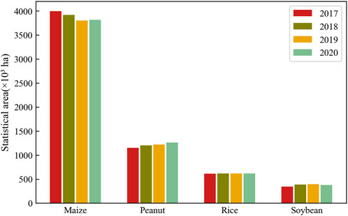
FIGURE 1. Statistical area of maize, peanut, rice, and soybean from 2017 to 2020 in Henan Province.

FIGURE 2

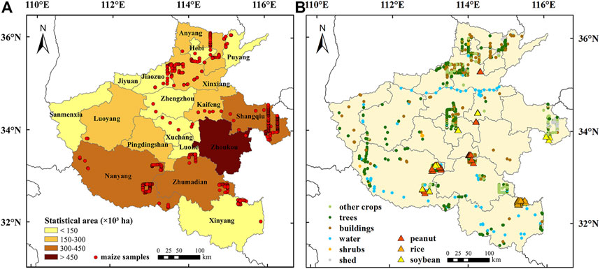
FIGURE 2. Location of the study area and the ground truth samples. (A) Map of statistical areas at the city level. The red dots indicate maize samples. (B) The other non-maize samples. The red, orange, and yellow triangles indicate peanut, rice, and soybean samples, respectively. Those samples collected through field surveys in 2019.

2.2 Data

2.2.1 Satellite data

The 30-m spatial resolution bands and indexes for the entire study area were obtained from the Sentinel-2 (S2) TOA product. S2 provides over 13 spectral bands with high temporal and spatial resolution. All bands and indexes used in the study had a spatial resolution of 30-m, with a median composite of 8-day temporal resolution. The cloud probability product provided by the Sentinel Hub (https://developers.google.com/earth-engine/datasets/catalog/COPERNICUS_S2_CLOUD_PROBABILITY) was used in the research to eliminate the impact of clouds on the S2 product. Pixels with a cloud probability higher than 50% were removed to obtain a cloud-free image. The data covered the entire maize growing season (137–289 days of year) in Henan Province from 2017 to 2020. Data filtering and gap filling were performed according to the following procedure. Linear equations were used to interpolate missing data based on adjacent observations to ensure that all pixels in the study area had the same length of time series (Zheng et al., 2022b). Then, a Savitzky-Golay (SG) filter with order set to 2 and window size set to 5 was applied in this study to capture the seasonal cycle of vegetation greenness to construct a smoothed time series (Chen et al., 2004). All pre-processing was done on the Google Earth Engine platform.

2.2.2 Field data and agriculture census data

The study used survey samples to obtain a standard curve for maize and other summer crops, which was also used to assess the accuracy of the distribution map. Survey samples obtained from field surveys. In 2019, field investigations were conducted in Henan Province, and various samples including maize, rice, peanut, soybean, other crops, forests, shrubs, water, buildings, and sheds were collected (Figure 2). The total number of samples was 2,481, including 890 maize samples and 1,591 non-maize samples. The county-level statistical data of Henan Province from 2017 to 2020 were obtained from the statistical yearbook of each city-level city (https://data.cnki.net/Area/Home/Index/D16). The study collected all county-level statistics that could be collected, including acreage in 104 counties in 2017–2018, 148 counties in 2019, and 113 counties in 2020.

2.3 Method

2.3.1 Revised time-weighted dynamic time warping

In this study, the method TWDTW proposed by Maus et al. (2016) and Dong et al. (2020) was used to generate the maize distribution map. TWDTW is an improved method of DTW, and the original DTW algorithm measures the dissimilarity between time series by aligning the minimum accumulated distance of two non-linear time series (we assume time series X is known maize pixel and series Y is unknown land cover pixel) to adjust the time dimension by warping the Y series to find the minimum modified path of the series X, which indicates the degree of dissimilarity between the two series. TWDTW is an improved method of DTW, which forces a time-weighted penalty to dissimilarity based on DTW and performs better classification accuracy. The logical TWDTW with open boundaries was used for time-weighted penalty in this study, which had a low penalty for small time warps and a significant cost for large time warps.

In this study, we created a mask based on NDVI that only the pixels with a value of NDVI greater than .3 at any time from 137 to 289 days of year (DOY) were used to classify. Then, 50 survey samples of maize (Figure 2) were randomly selected and averaged to obtain the standard curve for the seasonal variation of maize in Henan. The TWDTW method was used to calculate the dissimilarity of the time series from the standard curve for each pixel. When the dissimilarity was low, it indicated that the time series of the pixel was more similar to the standard curve and more likely to be planted maize. The dissimilarity values were calculated for all the pixels, and the pixels with dissimilarity values smaller than the threshold were identified as maize, and the area of all identified maize pixels was the same as the province-level statistical area (Dong et al., 2020; Zheng et al., 2022a).

On this basis, we revised the TWDTW method by combining two or more bands or indexes to classify. The details are shown in Figure 3. First, each identification got a distance matrix and a time weight matrix, summed up to get the cumulative distance matrix. Then, through the cumulative distance matrix, we calculate the minimum modified path of the time series Y (unknown land cover pixel) to the time series X (known maize pixel) to obtain the minimum distance value. The smaller the distance value, the more likely the unknown pixel planted maize. After all pixels were calculated, a minimum distance map was generated. Each band or index obtained a minimum distance map at their respective optimal phenological period (see Section 2.3.2). We sorted each minimum distance map to obtain a rank map, which can be considered as normalized dissimilarity map. Two or more rank maps were added together to obtain a new combined rank map. Finally, a new maize map identified from multiple bands or indexes was obtained through the threshold determined by the province-level statistical area.

FIGURE 3

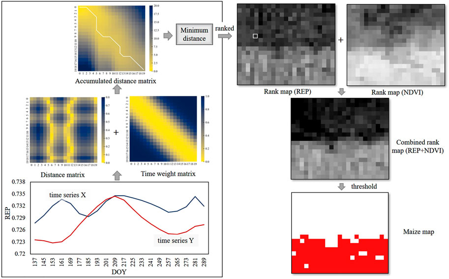
FIGURE 3. Process of the revised time-weighted dynamic time warping, using REP and NDVI as an example. The time series X is known maize pixel and the time series Y is unknown land cover pixel. The white line in the accumulated cost matrix is the optimal warping path between two sequences.

In this study, a total of ten spectral bands and three indexes derived from the S2 data were selected for maize identification (Figure 4). The ten bands of S2 included blue, green, red, red edge1 (RE1), red edge2 (RE2), red edge3 (RE3), red edge4 (RE4), near infrared (NIR), short wave infrared1 (SWIR1), and short wave infrared2 (SWIR2) (Table 1). The three spectral indexes were LSWI, red edge position index (REP), and NDVI, calculated using the following equation:

$\begin{array}{c}\mathit{L}\mathit{S}\mathit{W}\mathit{I}=\frac{{\mathit{\rho }}_{\mathit{N}\mathit{I}\mathit{R}}-{\mathit{\rho }}_{\mathit{S}\mathit{W}\mathit{I}\mathit{R}}}{{\mathit{\rho }}_{\mathit{N}\mathit{I}\mathit{R}}+{\mathit{\rho }}_{\mathit{S}\mathit{W}\mathit{I}\mathit{R}}}\end{array}(1)$

$\begin{array}{c}\mathit{R}\mathit{E}\mathit{P}=\mathbf{705}+\mathbf{35}\times \frac{\mathbf{0.5}\times \left({\mathit{\rho }}_{\mathit{R}\mathit{E}\mathbf{3}}+{\mathit{\rho }}_{\mathit{R}\mathit{e}\mathit{d}}\right)-{\mathit{\rho }}_{\mathit{R}\mathit{E}\mathbf{1}}}{{\mathit{\rho }}_{\mathit{R}\mathit{E}\mathbf{2}}-{\mathit{\rho }}_{\mathit{R}\mathit{E}\mathbf{1}}}\times \mathbf{100}\%\end{array}(2)$

$\begin{array}{c}\mathit{N}\mathit{D}\mathit{V}\mathit{I}=\frac{{\mathit{\rho }}_{\mathit{N}\mathit{I}\mathit{R}}-{\mathit{\rho }}_{\mathit{R}\mathit{e}\mathit{d}}}{{\mathit{\rho }}_{\mathit{N}\mathit{I}\mathit{R}}+{\mathit{\rho }}_{\mathit{R}\mathit{e}\mathit{d}}}\end{array}(3)$

where ${\rho }_{NIR}$, ${\rho }_{SWIR}$, ${\rho }_{Red}$, ${\rho }_{RE1}$, ${\rho }_{RE2}$, and ${\rho }_{RE3}$ are the top-of-atmosphere (TOA) reflectance values of the NIR, SWIR1, red, RE1, RE2, and RE3 of the S2 Multispectral Instrument (MSI).

FIGURE 4

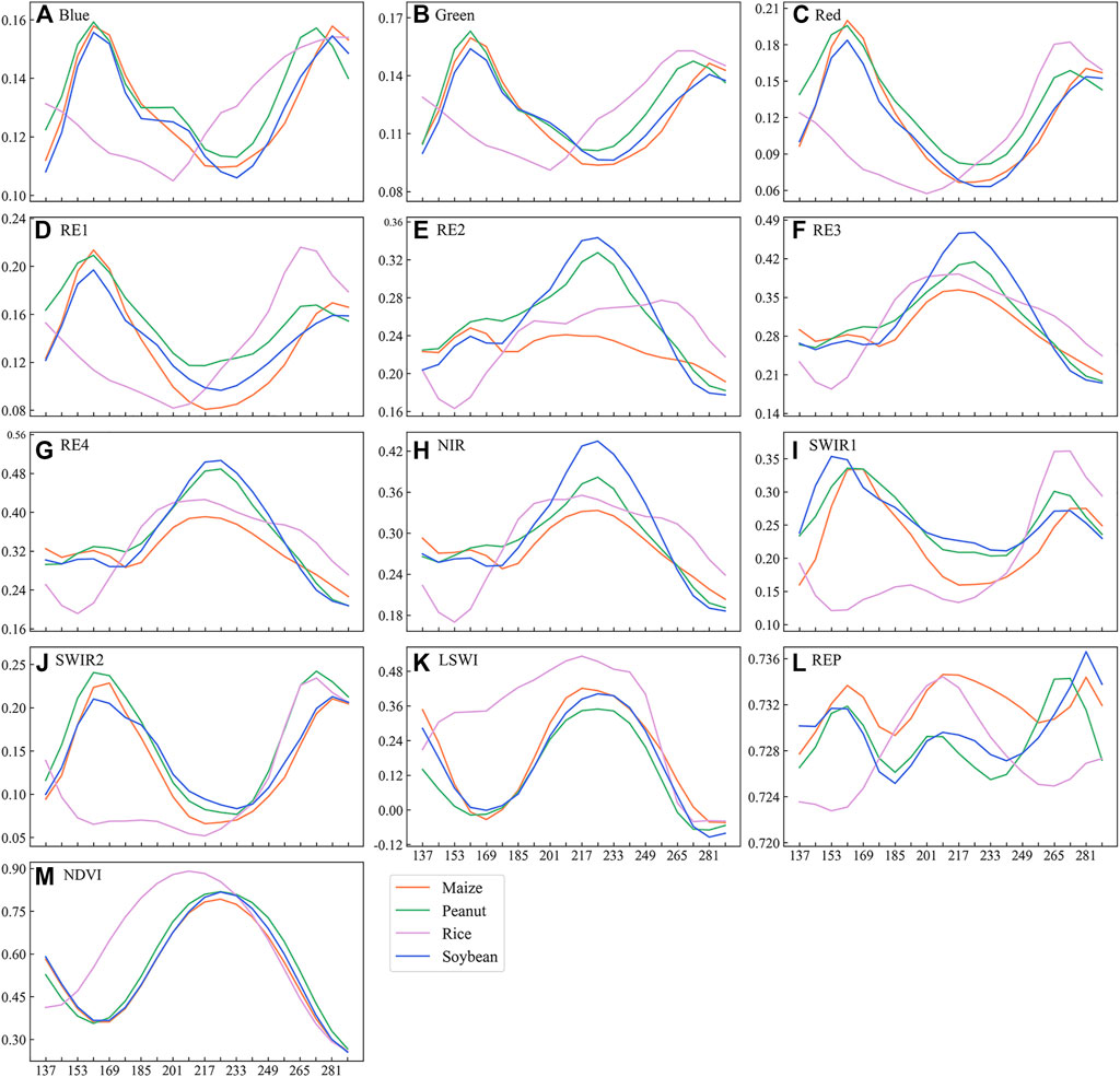
FIGURE 4. Standard seasonal curves of (A) blue, (B) green, (C) red, (D) RE1, (E) RE2, (F) RE3, (G) RE4, (H) NIR, (I) SWIR1, (J) SWIR2, (K) LSWI, (L) REP, and (M) NDVI for maize, peanut, rice, and soybean in Henan Province in 2019.

TABLE 1

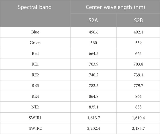
TABLE 1. Specifications of the Multispectral Instrument (MSI) bands on the Sentinel-2 A and B satellite systems.

2.3.2 Determination of phenology periods

We examined the key phenological periods of all ten bands and three indexes for distinguishing maize from the other summer crops. This study initially set the start date of the key phenological phase on the 137th day (May 5th), and the end date on the 289th day (October 10th). We used a time-sliding approach to investigate the best phenological periods of each band and index to classify maize with other summer crops. For each test, based on the standard curve of each band and index individually, we used the TWDTW method to identify maize planting area (see Section 2.3.1) and compare it with the county-level statistical area for verification. After comprehensively evaluating the R² and RMAE for each band or index during all potential phenological periods, we obtained the optimal time period of each band or index for maize mapping.

Taking REP as an example, the detailed steps are as follows (Figure 5): The size of the initial window (window₁ in Figure 5) is 8, with a total length of 64 days, and is slid from the left (DOY: 137–193) to the right (DOY: 233–289). The standard curve and the unknown time series in the corresponding time window are used to calculate the minimum distance value by TWDTW, and then derive a maize map based on a dissimilarity threshold. The size of the second window (window₂ in Figure 5) is 9, with a total length of 72 days, and the sliding steps are the same as above. The window size increases sequentially. The size of the last window (window₁₃ in Figure 5) is 20, a total of 160 days, covering the entire time period (DOY: 137–289). Each band or index experiences a total of 91 swipes, and each slide produces a maize map. Finally, a comprehensive evaluation by county-level validated R² and RMAE yields the optimal identification of the phenological period for each band and index.

FIGURE 5

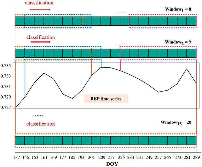
FIGURE 5. Time sliding taking REP as an example. The smallest window’s size is 8 (i.e., 64 days, window₁), and the largest window’s size is 20 (i.e., 160 days, window₁₃, DOY 137–289).

2.3.3 Accuracy assessment

First, we evaluated the coefficient of determination (R²) and relative mean absolute error (RMAE) of every band or index or combination. The calculation equations of R² and RMAE are as follows:

$\begin{array}{c}{\mathit{R}}^{\mathbf{2}}=1-\frac{{\displaystyle \sum }_{\mathit{i}=\mathbf{1}}^{\mathit{n}}{\left({\mathit{I}\mathit{A}}_{\mathit{i}}-{\mathit{S}\mathit{A}}_{\mathit{i}}\right)}^{\mathbf{2}}}{{\displaystyle \sum }_{\mathit{i}=\mathbf{1}}^{\mathit{n}}{\left(\overline{\mathit{S}\mathit{A}}-{\mathit{S}\mathit{A}}_{\mathit{i}}\right)}^{\mathbf{2}}}\end{array}(4)$

$\begin{array}{c}\mathit{R}\mathit{M}\mathit{A}\mathit{E}=\frac{{\displaystyle \sum }_{\mathit{i}=\mathbf{1}}^{\mathit{n}}\left|{\mathit{S}\mathit{A}}_{\mathit{i}}-{\mathit{I}\mathit{A}}_{\mathit{i}}\right|}{{\displaystyle \sum }_{\mathit{i}=\mathbf{1}}^{\mathit{n}}{\mathit{S}\mathit{A}}_{\mathit{i}}}\end{array}(5)$

where SA_i and IA_i are the statistical area and identified area of the ith county, and n indicates the amount of the counties in the given province.

Second, the classification accuracy was assessed based on field survey samples from 2019. Fifty random field samples were used to calculate the standard curve for maize, and the remaining 2,431 samples were set aside and used to calculate four accuracy metrics, including producer accuracy (PA), user accuracy (UA), overall accuracy (OA) and Kappa coefficient. PA represents the percentage of maize samples surveyed that are correctly identified as maize; UA represents the percentage of maize on the classification map that is actually confirmed by fieldwork; OA quantifies the overall effectiveness of the method and is calculated as the percentage of correctly identified samples. The Kappa coefficient (Congalton and Green, 1999) considers all samples of the confusion matrix and is used to analyze the level of consistency between the classification and the reference data. The four accuracies can be calculated as:

$\begin{array}{c}\mathbf{P}\mathbf{A}=\frac{\mathit{T}\mathit{P}}{\mathit{T}\mathit{P}+\mathit{F}\mathit{P}}\times \mathbf{100}\%\end{array}(6)$

$\begin{array}{c}\mathbf{U}\mathbf{A}=\frac{\mathit{T}\mathit{P}}{\mathit{T}\mathit{P}+\mathit{F}\mathit{N}}\times \mathbf{100}\%\end{array}(7)$

$\begin{array}{c}\mathbf{O}\mathbf{A}=\frac{\mathit{T}\mathit{P}+\mathit{T}\mathit{N}}{\mathit{T}\mathit{P}+\mathit{T}\mathit{N}+\mathit{F}\mathit{P}+\mathit{F}\mathit{N}}\times \mathbf{100}\%\end{array}(8)$

$\begin{array}{c}\mathbf{K}\mathbf{a}\mathbf{p}\mathbf{p}\mathbf{a}=\frac{{\mathit{P}}_{\mathit{o}}-{\mathit{P}}_{\mathit{e}}}{\mathbf{1}-{\mathit{P}}_{\mathit{e}}}\times \mathbf{100}\%\end{array}(9)$

where TP is the number of maize samples that are correctly classified. TN is the number of non-maize samples that are correctly classified. FP is the number of non-maize samples that are classified as maize. FN is the number of maize samples that are classified as non-maize. $P_o$ is the proportion of observed accuracy and $P_e$ is the proportion of expected accuracy.

3 Results

First, we examined the performance of a single satellite-based spectral band or index for identifying maize. In order to detect the best phenological periods of each band and index, we used a running window to generate all possible phenological periods starting from DOY 137 and ending to DOY 289 (see Section 2.3), and we compared the performance of each band and index with all potential phenological periods by comparing the identified areas with statistical area at county level. The results showed that almost the performance of all spectral bands and indexes largely varied during the different periods (Figure 6). For example, REP containing the DOY 233–289 showed the best performance than those during other periods (Figure 6L). Therefore, we compared the performance of each band and index with the best phenological periods. There were large differences in the performance of various bands and indexes compared to the statistical area (Table 2). In all investigated spectral bands and indexes, REP showed the best performance, and the identified areas showed the highest correlation with statistical areas (R² = .810) and the lowest RMAE (.343) (Table 2). In contrast, RE2 had the poorest performance with the R² of .575 and the RMAE of .415 (Table 2).

FIGURE 6

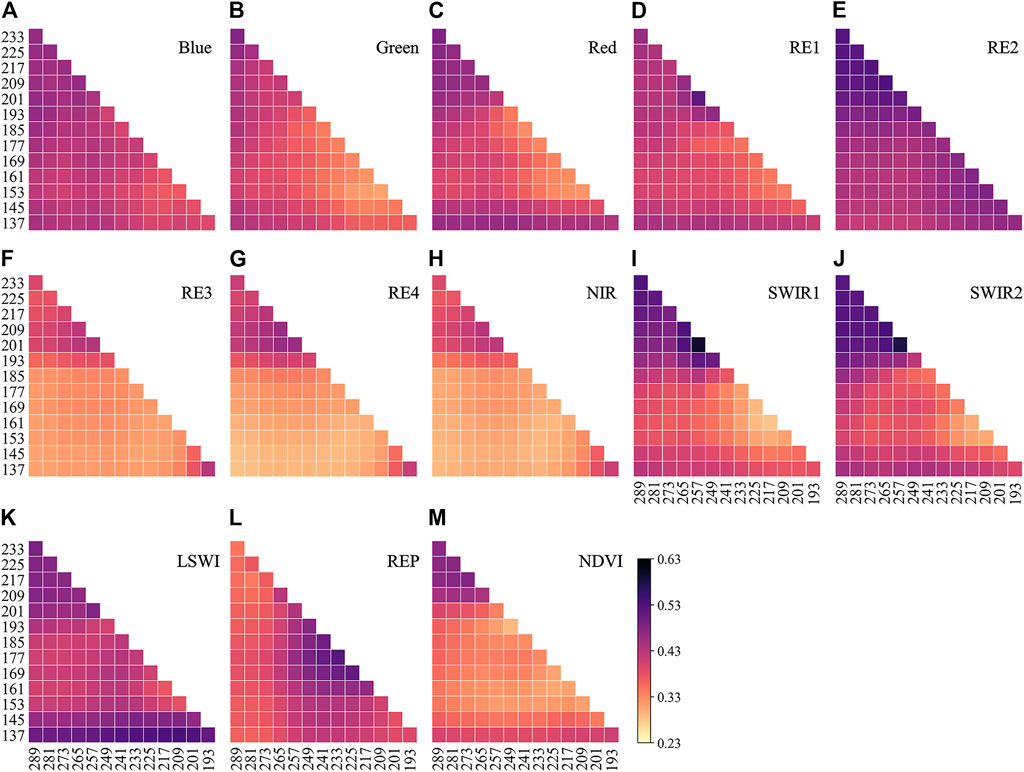
FIGURE 6. Comparison between statistical county-level maize cultivated area in 2019 with the identified area based on (A) blue, (B) green, (C) red, (D) RE1, (E) RE2, (F) RE3, (G) RE4, (H) NIR, (I) SWIR1, (J) SWIR2, (K) LSWI, (L) REP, and (M) NDVI during the all potential phenological periods. A total of 91 potential phenological periods for each band or index (Table 1).

TABLE 2

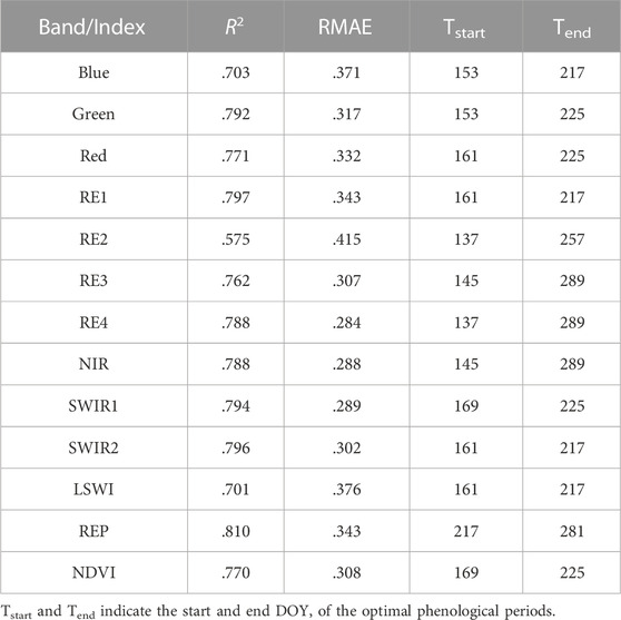
TABLE 2. Identification performance of each spectral band and index with the best phenological periods.

We further examined if the combinations of two bands or indexes can improve the identification accuracy compared to one single band or index, and the phenological periods of each band and index were set as the best phenological periods shown in Table 2. There are a total of 66 combinations of two bands or indexes. The results showed large differences in the identification accuracy of various combinations, such as R² ranging from .703 to .855 (Figure 7A). Most combinations outperformed the single band or index (Figures 7C, D). For example, the RMAE derived by the combination of NIR and SWIR2 decreased about 10% compared to the lower RMAE of one single band of these two bands (Figure 7D). On contrary, incorporating some bands or indexes will result in lower identification accuracy. It can be seen from Figure 7 that the combinations with LSWI showed worse accuracy. Most combinations with RE3, RE4, and NIR performed better (Figure 7A). The highest accuracy was achieved with the combination of SWIR2 and NIR, with R² of .855 and RMAE of .258; this was followed by the combination of SWIR2 and RE4, with R² of .853 and RMAE of .259 (Figures 7A, B).

FIGURE 7

FIGURE 7. Comparisons of the accuracy of a total of 66 combinations of two bands or indexes. (A,B) The R² and RMAE of maize planting area and statistical area on the county-level for 2019. (C,D) The difference of R² and RMAE between the combinations and the better single band or index in the combinations.

According to the above comparisons on combinations of two bands shown in Figure 7, the combinations with RE3, RE4, and NIR performed better than other combinations. Therefore, we further selected all combinations with these three bands to generate the combinations of three bands or indexes by integrating another band or index. The classification accuracy of most three bands or indexes combinations was not much improved compared to the two bands or indexes combinations (Figures 8C, D). The highest accuracy was achieved by the combination of NIR, SWIR2, and green, with R² of .856 and RMAE of .266; the second was with the combination of NIR, SWIR2, and red, whose accuracy is very close to the highest (R² = .856, RMAE = .273) (Figures 8A, B). Similarly, there was little improvement in the classification accuracy of the combinations of four bands or indexes, with a decrease in R² for almost all combinations, and an increase in RMAE for most combinations (Figures 9C, D). The above results indicated that as the number of bands or indexes in the combination increases to three or more, the accuracy (R² and RMAE) no longer increases.

FIGURE 8

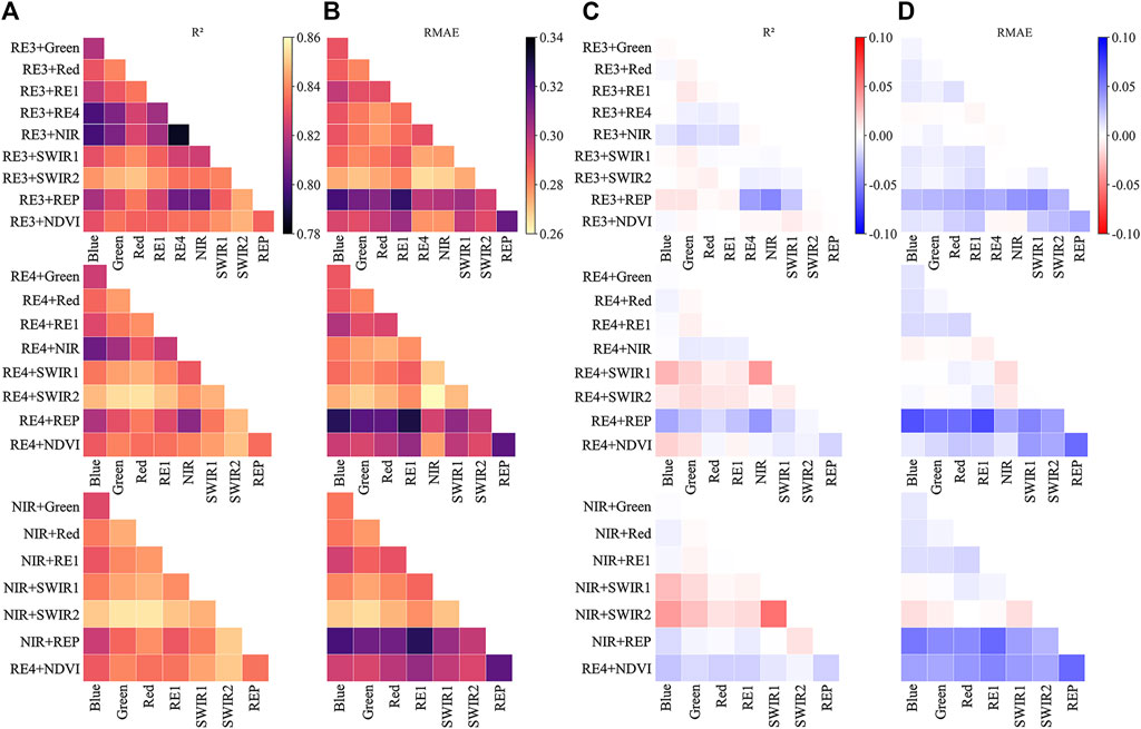
FIGURE 8. Comparisons of the accuracy of a total of 109 combinations of three bands or indexes. (A,B) R² and RMAE of maize planting area and statistical area on the county-level for 2019 in Henan. (C,D) Difference in R² and RMAE between the combinations of three and the combinations of two.

FIGURE 9

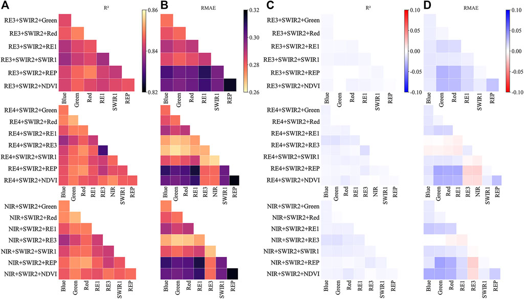
FIGURE 9. Comparisons of the accuracy of a total of 85 combinations of four bands or indexes. (A,B) The R² and RMAE of maize planting area and statistical area on the county-level for 2019 in Henan. (C,D) The difference of R² and RMAE between the combinations of four and the combinations of three.

To better verify the classification accuracy of each combination, we calculated the UA, PA, OA, and kappa using the field survey data in 2019. The accuracies of the maize maps were not identical using different bands or indexes. SWIR2 had the highest accuracy (OA 88.69%), followed by NDVI (OA 86.22%); while red (OA 79.68%) and REP (OA 75.24%) had much lower accuracies (Table 3). The combinations obtained significant improvements compared to the basic single band or index. For example, the combination of RE4 and SWIR2 increased OA up to 10.90% compared to RE4 and 3.08% compared to SWIR2. Besides, with the increase of the number of bands or indexes in the combination, the accuracy was also improved. The average OA of the two, three, and four bands or indexes combinations were 89.94%, 90.75%, and 92.07%, respectively. Finally, a comprehensive evaluation of R², RMAE and OA showed that the combination of RE4 and SWIR2 was the best among the 15 combinations tested in the study.

TABLE 3

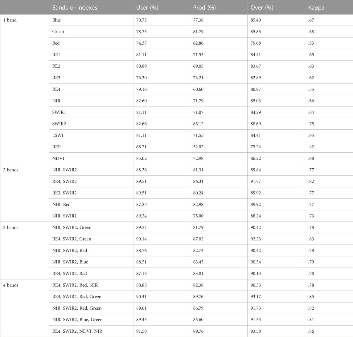
TABLE 3. Confusion matrices of combinations in 2019.

The combination of RE4 and SWIR2 was used for maize mapping in 2017–2020. At the county level, the identified maize area matched very well with the statistical area (Figure 10). The scatters were close to the 1:1 line, and the R² reached above .83 with RMAE lower than .27. The comparison of the maize map based on the combination of RE4 and SWIR2 with the very high-resolution images of maize from Google Earth showed high spatial consistency in the two regions (Figure 11) and was able to exclude buildings, roads and other crops, and only slightly misclassified some small areas.

FIGURE 10

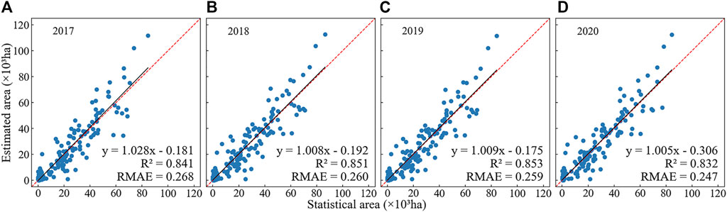
FIGURE 10. County-level comparison of identified and statistical planting areas in (A) 2017, (B) 2018, (C) 2019, and (D) 2020 in Henan Province. The solid lines indicate the 1:1 line, and the red dashed lines indicate the regression lines.

FIGURE 11

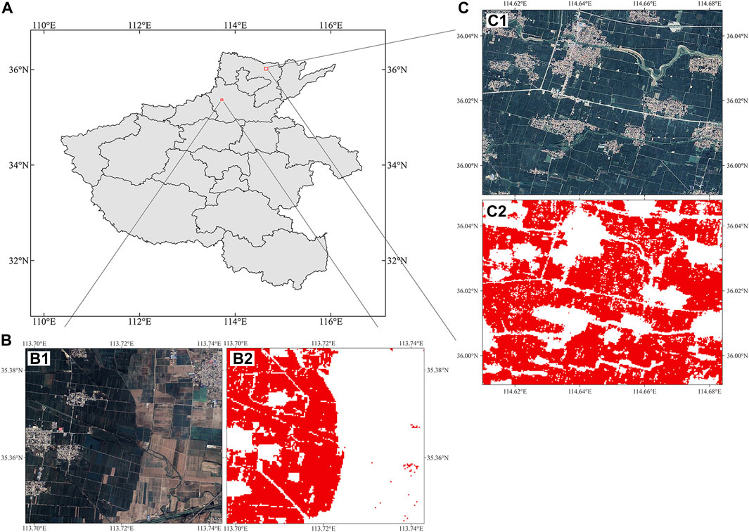
FIGURE 11. (A) The validation area is located in the north of Henan Province. (B1) and (C1) the very high-resolution image from ©Google Earth. (B2) and (C2) presence (red) and absence (white) of maize on the harvest map in 2019.

4 Discussion

It has been a significant challenge to identify summer crops because of similar phenology characteristics (de Souza et al., 2015; Wang et al., 2022). Multitemporal scenes of one single spectral band or index are commonly used for crop identification (Kussul et al., 2017; Ienco et al., 2019). Our results also showed the similar phenological characteristics among the four summer crops including maize, peanut, soybean, and rice (Figure 4). Therefore, it is quite difficult to map maize relying on a single band or index due to spectral confusion in summer crops. Even when two or more bands and indexes are input for training, phenological characteristics cannot be extracted effectively (Abubakar et al., 2020; You and Dong, 2020; Chen Y. et al., 2021). Previous methods usually used machine learning methods, and limited the application capability to the other regions (Rodriguez-Galiano et al., 2012).

In this study, a multi-band recognition attempt was conducted based on the TWDTW algorithm. The results showed that the combinations of two and more bands and indexes can effectively improve the identification performance compared to one single band or index (Figures 7–9). One of the most important theory basics is large sensitivity differences of various crops to different spectral bands or indexes (Yin et al., 2020; Zhao et al., 2020). Studies have found that the reflectance in the red edge region is mainly affected by leaf absorption and canopy scattering (Baret et al., 1994; Yang and van der Tol, 2018). For the same total leaf chlorophyll content, absorption of a maize leaf in the red edge region is the same as that of a soybean leaf (Peng and Gitelson, 2012). But the scattering of a spherical canopy (soybean) is higher than that of a heliotropic canopy (maize) (Nguy-Robertson et al., 2012). Therefore, the RE4 reflectance of maize is lower than that of soybean (Peng et al., 2011). And the leaf reflectance of peanut in the red edge regions is very close to that of soybean (Buchaillot et al., 2022). SWIR2, another member of the best combination, is very sensitive to changes in soil moisture (Khanna et al., 2007). The differences between maize and paddy rice are striking during the irrigated period of paddy rice, with a much lower value of SWIR2 in paddy rice than in maize (Figure 4).

The new method also highlighted the importance of selecting phenological periods for spectral bands. In general, the classification accuracy of the TWDTW classifiers depends on the distinguishability of the temporal profiles of different crops (Gella et al., 2021). This study examined the difference in the phenological periods of each band or index for identifying maize, and only one band (RE4) showed the best performance using the temporal variations during the entire growing periods, whereas the other bands or indexes are better in certain phenological stages. For example, LSWI, SWIR1 and SWIR2 performed the best during DOY 161–225 (early and middle growth stage) (Table 2), adding data acquired in the late period (DOY 233–289) only brings information redundancy, which has little effect on improving classification accuracy. This phenomenon was also observed by Jia et al. (2012) when they investigated the ability of SAR data in the North China Plain to classify crops. They found that the information contained in two temporal SAR datasets acquired in late jointing and flowering periods is enough for crop classification; Sun et al. (2019) extracted different temporal features to identify crops, and found that the classification accuracy varies widely. In May (flowering period), the crops obtained the best OA and kappa. Research showed that rather than using the entire phenological period, images of optimal time periods can achieve higher classification accuracy (Murakami et al., 2001; Hao et al., 2015).

According to the validation using field surveys and statistical area at county level, this study showed the good performance of the new method for identifying maize. In addition, we also investigated the temporal and spatial patterns of identified maize, which are another important information for judging the method reliability (Pan et al., 2021; Zheng et al., 2022b). The study area (i.e., Henan Province) is one of the largest contributors of maize production in China (Shen et al., 2022), and there are large areas to continuously plant maize (Zhang et al., 2018). The results of the combination of RE4 and SWIR2 showed that more than 95% of fields have been planted maize for four continuous years (Figure 12C). However, single-band RE4 and SWIR2 could not reflect the characteristics of large-scale continuous maize cultivation in Henan Province (Figures 12A, B). In addition, previous studies highlighted that satellite-based classification may result in “salt-and-pepper” noise, i.e., large amounts of isolated single or small area patches consisted of identified maize pixels (Zheng et al., 2022a). Our results indicated a high proportion of isolated large patches of identified maize (Figure 12D). Especially, compared to the classification map based on one single band or index, there are lower proportion of small area patches.

FIGURE 12

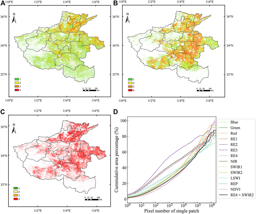
FIGURE 12. The planting frequency of maize in Henan Province from 2017 to 2020 by (A) RE4, (B) SWIR2, and (C) the combination of RE4 and SWIR2. The number 1–4 means that maize planted for continuous one to four investigated years. And (D) Statistics for patches with different pixel numbers in the maize harvest map for Henan in 2019, including the ten spectral bands, three indexes and the combination of RE4 and SWIR2.

Nowadays, the world is in a rapid stage of agricultural modernization, but food security remains a top priority. Maize is one of the most widely produced cereals in the world and can be used for human food, livestock feed, and bioenergy (Ranum et al., 2014). Accurate and timely information of maize acreage is critical for regional and global food security as well as international food trade. The high-resolution crop distribution map can not only be used as a base map to predict crop production and improve the accuracy of large-scale crop yield simulations (Becker-Reshef et al., 2010; Franch et al., 2015; Wang S. et al., 2020), but also be used as a reference to predict its future planting distribution (Chu et al., 2021). Furthermore, agriculture has the unique potential to provide a beneficial contribution to the global carbon budget. For example, agriculture produces large amounts of nitrogen, one of the long-lived greenhouse gases, due to the use of fertilizers such as nitrogen fertilizers (Northrup et al., 2021; Pan et al., 2022). To better understand food security and greenhouse gas emissions, high spatial-resolution cropland area monitoring is necessary. Our improved method, the TWDTW method that combines multi-source data and phenological information, is suitable for the identification of common summer crops and can be extended to other regions. The produced maps can help to dynamically understand the planting distribution of summer crops, and can greatly help policy decisions related to agriculture and emission reduction.

Although our results showed robust classification by the new method, there are still some uncertainties that need to be resolved in the future. First, optical satellite remote sensing data are affected by clouds and rain, and there were few effective images in central Henan Province, especially in 2017 (Figure 13). While our algorithm screens for good-quality observations, data gaps due to persistent cloud cover create difficulties identifying crop cycles. Some fields may be mistakenly classified as non-maize. To address this, we need more remote sensing data with higher spatial and temporal resolution; another approach is to rely on the fusion of multi-source remote sensing data to produce products with high spatial and temporal resolution (Li et al., 2017; Zhu et al., 2017). In addition, another limitation comes from the impact of composite planting structures (Ghosh et al., 2006; Maitra et al., 2021). The regular maize-soybean strip intercropping, originally popularized in northern China, and maize-soybean relay-strip intercropping extended in southwestern China (Du et al., 2018), generating more complex phenological characteristics. A flexible utilization of the phenological period with TWDTW may be able to better deal with these issues.

FIGURE 13

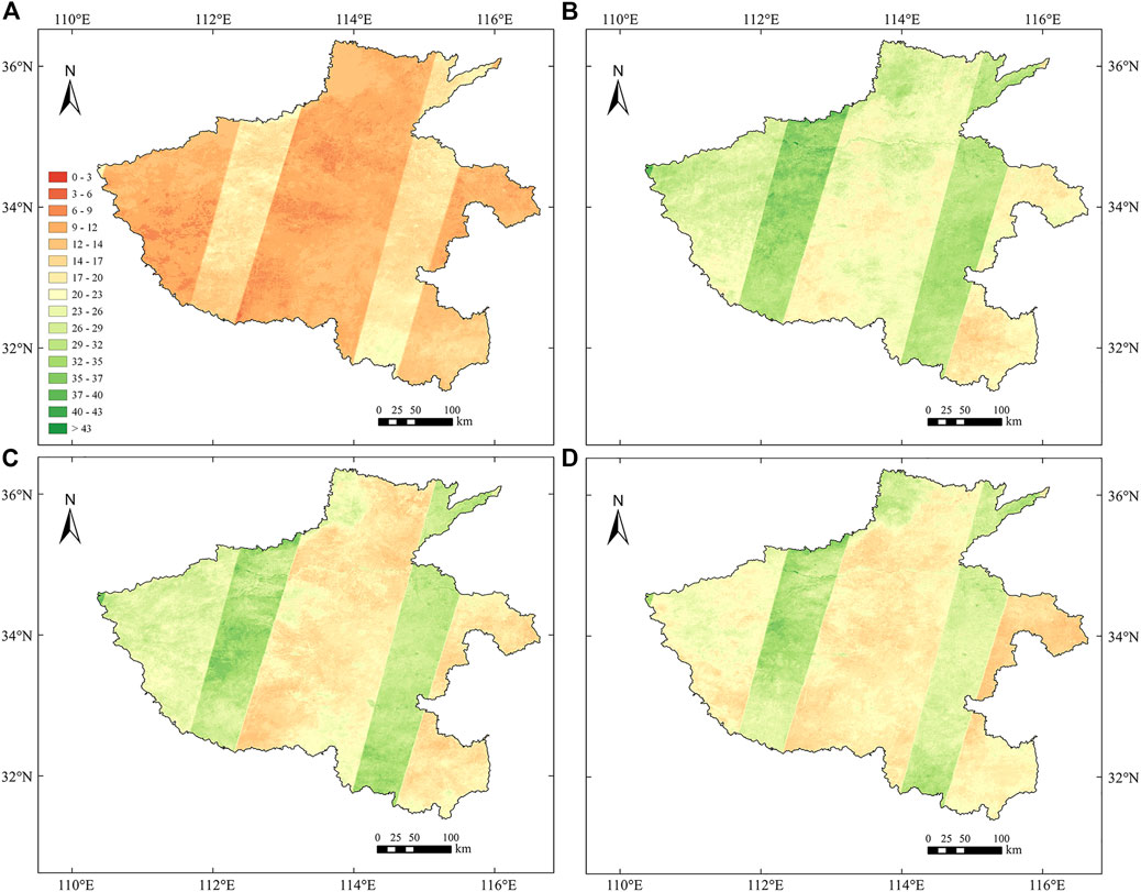
FIGURE 13. Times of good observations of 8-day maximum NDVI composite images during the maize growing season of (A) 2017; (B) 2018; (C) 2019; and (D) 2020.

5 Conclusion

This study developed a new phenological-based method to identify the summer crop based on multiple bands with their specific phenological periods. As an example, this study examined the performance of this new method for identifying maize in Henan Province of China. Ten spectral bands and three synthetic indexes derived from the Sentinel-2 dataset were used based on the revised TWDTW method. Time sliding was first performed on all bands and indexes with different time window sizes on 137–289 days of year to obtain the best identification phenological periods. On this basis, the performance of the multi-band combination TWDTW method in extracting maize planting area was evaluated. The combination of RE4 and SWIR2 had the best performance among all combinations, with overall classification accuracy reaching 91.77%. A total of more than 100 counties were selected for data accuracy assessment from 2017 to 2020, showing that the maize planting area estimated by this combination correlated well with the statistical data, with R² greater than .83 and RMAE lower than .27. The combined effect was more accurate than for all single bands; with the increase in the number of bands or indexes in the combination, the overall classification accuracy improved with the use of up to three bands. The results indicated a robust potential for combining multiple bands or indexes and crop phenological information using the TWDTW method in the application of maize planting area monitoring.

Data availability statement

The original contributions presented in the study are included in the article/supplementary material, further inquiries can be directed to the corresponding author.

Author contributions

QP and RS contributed to conception and design of the study. WY provided theoretical guidance. QP conducted the statistical analysis and wrote the first draft of the manuscript. WY reviewed and edited the manuscript. Field data collection was conducted by JD and WH. JH, TY, and WZ supervised the study. All authors contributed to manuscript revision, read, and approved the submitted version.

Funding

This study was supported by the National Science Fund for Distinguished Young Scholars (41925001).

Conflict of interest

The authors declare that the research was conducted in the absence of any commercial or financial relationships that could be construed as a potential conflict of interest.

Publisher’s note

All claims expressed in this article are solely those of the authors and do not necessarily represent those of their affiliated organizations, or those of the publisher, the editors and the reviewers. Any product that may be evaluated in this article, or claim that may be made by its manufacturer, is not guaranteed or endorsed by the publisher.

References

Abubakar, G. A., Wang, K., Shahtahamssebi, A., Xue, X., Belete, M., Gudo, A. J. A., et al. (2020). Mapping maize fields by using multi-temporal sentinel-1A and sentinel-2A images in makarfi, northern Nigeria, africa. Afr. Sustain. 12, 2539. doi:10.3390/su12062539

CrossRef Full Text | Google Scholar

Arvor, D., Jonathan, M., Meirelles, M. S. P., Dubreuil, V., and Durieux, L. (2011). Classification of MODIS EVI time series for crop mapping in the state of Mato Grosso, Brazil. Braz. Int. J. Remote Sens. 32, 7847–7871. doi:10.1080/01431161.2010.531783

CrossRef Full Text | Google Scholar

Ashourloo, D., Shahrabi, H. S., Azadbakht, M., Aghighi, H., Nematollahi, H., Alimohammadi, A., et al. (2019). Automatic canola mapping using time series of sentinel 2 images. ISPRS J. Photogrammetry Remote Sens. 156, 63–76. doi:10.1016/j.isprsjprs.2019.08.007

CrossRef Full Text | Google Scholar

Baret, F., Vanderbilt, V. C., Steven, M. D., and Jacquemoud, S. (1994). Use of spectral analogy to evaluate canopy reflectance sensitivity to leaf optical properties. Sens. Environ. 48, 253–260. doi:10.1016/0034-4257(94)90146-5

CrossRef Full Text | Google Scholar

Becker-Reshef, I., Vermote, E., Lindeman, M., and Justice, C. (2010). A generalized regression-based model for forecasting winter wheat yields in Kansas and Ukraine using MODIS data. Remote Sens. Environ. 114, 1312–1323. doi:10.1016/j.rse.2010.01.010

CrossRef Full Text | Google Scholar

Belgiu, M., Bijker, W., Csillik, O., and Stein, A. (2021). Phenology-based sample generation for supervised crop type classification. Int. J. Appl. Earth Observation Geoinformation 95, 102264. doi:10.1016/j.jag.2020.102264

CrossRef Full Text | Google Scholar

Belgiu, M., and Csillik, O. (2018). Sentinel-2 cropland mapping using pixel-based and object-based time-weighted dynamic time warping analysis. Sens. Environ. 204, 509–523. doi:10.1016/j.rse.2017.10.005

CrossRef Full Text | Google Scholar

Boryan, C., Yang, Z., Mueller, R., and Craig, M. (2011). Monitoring US agriculture: The US department of agriculture, national agricultural statistics Service, cropland data layer program. Crop. data Layer. program Geocarto Int. 26, 341–358. doi:10.1080/10106049.2011.562309

CrossRef Full Text | Google Scholar

Buchaillot, M. L., Soba, D., Shu, T., Liu, J., Aranjuelo, I., Araus, J. L., et al. (2022). Estimating peanut and soybean photosynthetic traits using leaf spectral reflectance and advance regression models. Planta 255, 93. doi:10.1007/s00425-022-03867-6

PubMed Abstract | CrossRef Full Text | Google Scholar

Carletto, C., Gourlay, S., and Winters, P. (2015). From guesstimates to gpstimates: Land area measurement and implications for agricultural analysis. J. Afr. Econ. 24, 593–628. doi:10.1093/jae/ejv011

CrossRef Full Text | Google Scholar

Chen, H., Chen, C., Zhang, Z., Lu, C., Wang, L., He, X., et al. (2021). Changes of the spatial and temporal characteristics of land-use landscape patterns using multi-temporal landsat satellite data: A case study of zhoushan island, China. Ocean Coast. Manag. 213, 105842. doi:10.1016/j.ocecoaman.2021.105842

CrossRef Full Text | Google Scholar

Chen, J., Jönsson, P., Tamura, M., Gu, Z., Matsushita, B., Eklundh, L., et al. (2004). A simple method for reconstructing a high-quality ndvi time-series data set based on the savitzky–golay filter. Remote Sens. Environ. 91, 332–344. doi:10.1016/s0034-4257(04)00080-x

CrossRef Full Text | Google Scholar

Chen, Y., Hou, J., Huang, C., Zhang, Y., and Li, X. (2021). Mapping maize area in 1heterogeneous agricultural landscape with multi-temporal sentinel-1 and sentinel-2 images based on random forest. Remote Sens. 13, 2988. doi:10.3390/rs13152988

CrossRef Full Text | Google Scholar

Cheng, K., and Wang, J. (2019). Forest-Type classification using time-weighted dynamic time warping analysis in mountain areas: A case study in southern China. A case study South. china For. 10, 1040. doi:10.3390/f10111040

CrossRef Full Text | Google Scholar

Chew, R., Rineer, J., Beach, R., O’Neil, M., Ujeneza, N., Lapidus, D., et al. (2020). Deep neural networks and transfer learning for food crop identification in uav images. Drones 4, 7. doi:10.3390/drones4010007

CrossRef Full Text | Google Scholar

Chu, L., Jiang, C., Wang, T., Li, Z., and Cai, C. (2021). Mapping and forecasting of rice cropping systems in central China using multiple data sources and phenology-based time-series similarity measurement. Adv. Space Res. 68, 3594–3609. doi:10.1016/j.asr.2021.06.053

CrossRef Full Text | Google Scholar

Congalton, R. G., and Green, K. (1999). Assessing the accuracy of remotely sensed data: Principles and practices, 43–70. Boca Raton, FL: Lewis Publishers.

PubMed Abstract | Google Scholar

Crane-Droesch, A. (2018). Machine learning methods for crop yield prediction and climate change impact assessment in agriculture. Environ. Res. Lett. 13, 114003. doi:10.1088/1748-9326/aae159

CrossRef Full Text | Google Scholar

de Souza, C. H. W., Mercante, E., Johann, J. A., Lamparelli, R. A. C., and Uribe-Opazo, M. A. (2015). Mapping and discrimination of soya bean and corn crops using spectro-temporal profiles of vegetation indices. Int. J. Remote Sens. 36, 1809–1824. doi:10.1080/01431161.2015.1026956

CrossRef Full Text | Google Scholar

Dong, J., Fu, Y., Wang, J., Tian, H., Fu, S., Niu, Z., et al. (2020). Early-season mapping of winter wheat in China based on landsat and sentinel images. Earth Syst. Sci. Data 12, 3081–3095. doi:10.5194/essd-12-3081-2020

CrossRef Full Text | Google Scholar

Dong, J., Xiao, X., Kou, W., Qin, Y., Zhang, G., Li, L., et al. (2015). Tracking the dynamics of paddy rice planting area in 1986–2010 through time series landsat images and phenology-based algorithms. Remote Sens. Environ. 160, 99–113. doi:10.1016/j.rse.2015.01.004

CrossRef Full Text | Google Scholar

Du, J., Han, T., Gai, J., Yong, T. w., Sun, X., Wang, X. c., et al. (2018). Maize-soybean strip intercropping: Achieved a balance between high productivity and sustainability. J. Integr. Agric. 17, 747–754. doi:10.1016/s2095-3119(17)61789-1

CrossRef Full Text | Google Scholar

Fan, H., Fu, X., Zhang, Z., and Wu, Q. (2015). Phenology-based vegetation index differencing for mapping of rubber plantations using landsat oli data. Remote Sens. 7, 6041–6058. doi:10.3390/rs70506041

CrossRef Full Text | Google Scholar

FAO (2021). World food and agriculture - statistical yearbook 2021. Rome. doi:10.4060/cb4477en

CrossRef Full Text | Google Scholar

Food and Agriculture Organization, (2017). Online statistical database: Trade. Available at: http://faostat.fao.org/(Accessed Nov 24, 2022).

Google Scholar

Franch, B., Vermote, E. F., Becker-Reshef, I., Claverie, M., Huang, J., Zhang, J., et al. (2015). Improving the timeliness of winter wheat production forecast in the United States of America, Ukraine and China using MODIS data and NCAR Growing Degree Day information. Remote Sens. Environ. 161, 131–148. doi:10.1016/j.rse.2015.02.014

CrossRef Full Text | Google Scholar

Fu, Y., Huang, J., Shen, Y., Liu, S., Dong, J., Han, W., et al. (2021). A satellite-based method for national winter wheat yield estimating in China. Remote Sens. 13, 4680. doi:10.3390/rs13224680

CrossRef Full Text | Google Scholar

Geerken, R. A. (2009). An algorithm to classify and monitor seasonal variations in vegetation phenologies and their inter-annual change. ISPRS J. Photogrammetry Remote Sens. 64, 422–431. doi:10.1016/j.isprsjprs.2009.03.001

CrossRef Full Text | Google Scholar

Gella, G. W., Bijker, W., and Belgiu, M. (2021). Mapping crop types in complex farming areas using sar imagery with dynamic time warping. ISPRS J. Photogrammetry Remote Sens. 175, 171–183. doi:10.1016/j.isprsjprs.2021.03.004

CrossRef Full Text | Google Scholar

Ghosh, P. K., Manna, M. C., Bandyopadhyay, K. K., Ajay,, , Tripathi, A. K., Wanjari, R. H., et al. (2006). Interspecific interaction and nutrient use in soybean/sorghum intercropping system. Journal 98, 1097–1108. doi:10.2134/agronj2005.0328

CrossRef Full Text | Google Scholar

Guo, Y., Xia, H., Pan, L., and Zhao, X. (2022). Mapping the northern limit of double cropping using a phenology-based algorithm and Google Earth engine. Remote Sens. 14, 1004. doi:10.3390/rs14041004

CrossRef Full Text | Google Scholar

Hamada, M. A., Kanat, Y., and Abiche, A. E.Department of IS, IIT University, Almaty KazakhstanSenior Lecturer in Computer & Information Security, IITU Almaty, Kazakhstan. (2019). Multi-spectral image segmentation based on the k-means clustering. IJITEE 9, 1016–1019. doi:10.35940/ijitee.k1596.129219

CrossRef Full Text | Google Scholar

Hao, P., Zhan, Y., Wang, L., Niu, Z., and Shakir, M. (2015). Feature selection of time series modis data for early crop classification using random forest: A case study in Kansas, USA. Remote Sens. 7 (5), 5347–5369. doi:10.3390/rs70505347

CrossRef Full Text | Google Scholar

Hoekman, D. H., and Vissers, M. A. M. (2003). A new polarimetric classification approach evaluated for agricultural crops. IEEE Trans. Geoscience Remote Sens. 41, 2881–2889. doi:10.1109/tgrs.2003.817795

CrossRef Full Text | Google Scholar

Huang, X., Fu, Y., Wang, J., Dong, J., Zheng, Y., and Pan, B. (2022). High-resolution mapping of winter cereals in Europe by time series landsat and sentinel images for 2016–2020. Remote Sens. 14, 2120. doi:10.3390/rs14092120

CrossRef Full Text | Google Scholar

Ienco, D., Interdonato, R., Gaetano, R., and Ho Tong Minh, D. (2019). Combining sentinel-1 and sentinel-2 satellite image time series for land cover mapping via a multi-source deep learning architecture. ISPRS J. Photogrammetry Remote Sens. 158, 11–22. doi:10.1016/j.isprsjprs.2019.09.016

CrossRef Full Text | Google Scholar

Inglada, J., Arias, M., Tardy, B., Hagolle, O., Valero, S., Morin, D., et al. (2015). Assessment of an operational system for crop type map production using high temporal and spatial resolution satellite optical imagery. Remote Sens. 7, 12356–12379. doi:10.3390/rs70912356

CrossRef Full Text | Google Scholar

Jia, K., Li, Q., Tian, Y., Wu, B., Zhang, F., and Meng, J. (2012). Crop classification using multi-configuration sar data in the north China plain. Int. J. Remote Sens. 33, 170–183. doi:10.1080/01431161.2011.587844

CrossRef Full Text | Google Scholar

Khanna, S., Palacios-Orueta, A., Whiting, M. L., Ustin, S. L., Riano, D., and Litago, J. (2007). Development of angle indexes for soil moisture estimation, dry matter detection and land-cover discrimination. Remote Sens. Environ. 109, 154–165. doi:10.1016/j.rse.2006.12.018

CrossRef Full Text | Google Scholar

Kussul, N., Lavreniuk, M., Skakun, S., and Shelestov, A. (2017). Deep learning classification of land cover and crop types using remote sensing data. IEEE Geoscience Remote Sens. Lett. 14, 778–782. doi:10.1109/lgrs.2017.2681128

CrossRef Full Text | Google Scholar

Li, L., Zhao, Y., Fu, Y., Pan, Y., Yu, L., and Xin, Q. (2017). High resolution mapping of cropping cycles by fusion of landsat and modis data. Remote Sens. 9, 1232. doi:10.3390/rs9121232

CrossRef Full Text | Google Scholar

Liu, J., Zhu, W., Atzberger, C., Zhao, A., Pan, Y., and Huang, X. (2018). A phenology-based method to map cropping patterns under a wheat-maize rotation using remotely sensed time-series data. Remote Sens. 10 (8), 1203. doi:10.3390/rs10081203

CrossRef Full Text | Google Scholar

Liu, W., Huang, J. F., Wei, C., Wang, X., Lamin, R., Han, J., et al. (2018). Mapping water-logging damage on winter wheat at parcel level using high spatial resolution satellite data. ISPRS J. Photogrammetry Remote Sens. 142, 243–256. doi:10.1016/j.isprsjprs.2018.05.024

CrossRef Full Text | Google Scholar

Löw, F., Michel, U., Dech, S., and Conrad, C. (2013). Impact of feature selection on the accuracy and spatial uncertainty of per-field crop classification using support vector machines. ISPRS J. Photogrammetry Remote Sens. 85, 102–119. doi:10.1016/j.isprsjprs.2013.08.007

CrossRef Full Text | Google Scholar

Maitra, S., Hossain, A., Brestic, M., Skalicky, M., Ondrisik, P., Gitari, H., et al. (2021). Intercropping—a low input agricultural strategy for food and environmental security. Intercropping—a low input Agric. strategy food Environ. Secur. Agron. 11, 343. doi:10.3390/agronomy11020343

CrossRef Full Text | Google Scholar

Maus, V., Câmara, G., Cartaxo, R., Sanchez, A., Ramos, F. M., and de Queiroz, G. R. (2016). A time-weighted dynamic time warping method for land-use and land-cover mapping. IEEE J. Sel. Top. Appl. Earth Observations Remote Sens. 9, 3729–3739. doi:10.1109/jstars.2016.2517118

CrossRef Full Text | Google Scholar

Millard, K., and Richardson, M. (2015). On the importance of training data sample selection in random forest image classification: A case study in peatland ecosystem mapping. Remote Sens. 7, 8489–8515. doi:10.3390/rs70708489

CrossRef Full Text | Google Scholar

Mohammadi, A., Khoshnevisan, B., Venkatesh, G., and Eskandari, S. (2020). A critical review on advancement and challenges of biochar application in paddy fields: Environmental and life cycle cost analysis. Environ. life cycle cost analysis Process. 8, 1275. doi:10.3390/pr8101275

CrossRef Full Text | Google Scholar

Moola, W. S., Bijker, W., Belgiu, M., and Li, M. (2021). Vegetable mapping using fuzzy classification of dynamic time warping distances from time series of sentinel-1a images. Int. J. Appl. Earth Observation Geoinformation 102, 102405. doi:10.1016/j.jag.2021.102405

CrossRef Full Text | Google Scholar

Murakami, T., Ogawa, S., Ishitsuka, N., Kumagai, K., and Saito, G. (2001). Crop discrimination with multitemporal SPOT/HRV data in the Saga Plains, Japan. Jpn. Int. J. Remote Sens. 22, 1335–1348. doi:10.1080/01431160151144378

CrossRef Full Text | Google Scholar

Nguy-Robertson, A., Gitelson, A., Peng, Y., Viña, A., Arkebauer, T., and Rundquist, D. (2012). Green leaf area index estimation in maize and soybean: Combining vegetation indices to achieve maximal sensitivity Agronomy. Journal 104, 1336–1347.

CrossRef Full Text | Google Scholar

Northrup, D. L., Basso, B., Wang, M. Q., Morgan, C. L. S., and Benfey, P. N. (2021). Novel technologies for emission reduction complement conservation agriculture to achieve negative emissions from row-crop production. Proc. Natl. Acad. Sci. U.S.A. 118, e2022666118. doi:10.1073/pnas.2022666118

PubMed Abstract | CrossRef Full Text | Google Scholar

Pan, B., Zheng, Y., Ye, T., Zhao, W., Dong, J., et al. (2021). High resolution distribution dataset of double-season paddy rice in China. J. Remote Sens. 13 (22). doi:10.3390/rs13224609

CrossRef Full Text | Google Scholar

Pan, S.-Y., He, K.-H., Lin, K.-T., Fan, C., and Chang, C.-T. (2022). Addressing nitrogenous gases from croplands toward low-emission agriculture. npj Clim. Atmos. Sci. 5, 43. doi:10.1038/s41612-022-00265-3

CrossRef Full Text | Google Scholar

Peña-Barragán, J. M., Ngugi, M. K., Plant, R. E., and Six, J. (2011). Object-based crop identification using multiple vegetation indices, textural features and crop phenology. Remote Sens. Environ. 115, 1301–1316. doi:10.1016/j.rse.2011.01.009

CrossRef Full Text | Google Scholar

Peng, Y., Gitelson, A. A., Keydan, G., Rundquist, D. C., and Moses, W. (2011). Remote estimation of gross primary production in maize and support for a new paradigm based on total crop chlorophyll content. Sens. Environ. 115, 978–989. doi:10.1016/j.rse.2010.12.001

CrossRef Full Text | Google Scholar

Peng, Y., and Gitelson, A. A. (2012). Remote estimation of gross primary productivity in soybean and maize based on total crop chlorophyll content. Sens. Environ. 117, 440–448. doi:10.1016/j.rse.2011.10.021

CrossRef Full Text | Google Scholar

Petitjean, F., Inglada, J., and Gancarski, P. (2012). Satellite image time series analysis under time warping. IEEE Trans. Geoscience Remote Sens. 50, 3081–3095. doi:10.1109/tgrs.2011.2179050

CrossRef Full Text | Google Scholar

Qiu, B., Jiang, F., Chen, C., Tang, Z., Wu, W., and Berry, J. (2021). Phenology-pigment based automated peanut mapping using sentinel-2 images. GIScience Remote Sens. 58, 1335–1351. doi:10.1080/15481603.2021.1987005

CrossRef Full Text | Google Scholar

Rad, A. M., Ashourloo, D., Shahrabi, H. S., and Nematollahi, H. (2019). Developing an automatic phenology-based algorithm for rice detection using sentinel-2 time-series data. IEEE J. Sel. Top. Appl. Earth Observations Remote Sens. 12, 1471–1481. doi:10.1109/jstars.2019.2906684

CrossRef Full Text | Google Scholar

Ranum, P., Peña-Rosas, J. P., and Garcia-Casal, M. N. (2014). Global maize production, utilization, and consumption. Ann. N. Y. Acad. Sci. 1312, 105–112. doi:10.1111/nyas.12396

PubMed Abstract | CrossRef Full Text | Google Scholar

Rao, N. R. (2008). Development of a crop-specific spectral library and discrimination of various agricultural crop varieties using hyperspectral imagery. Int. J. Remote Sens. 29, 131–144. doi:10.1080/01431160701241779

CrossRef Full Text | Google Scholar

Rodriguez-Galiano, V. F., Ghimire, B., Rogan, J., Chica-Olmo, M., and Rigol-Sanchez, J. (2012). An assessment of the effectiveness of a random forest classifier for land-cover classification. ISPRS J. Photogrammetry Remote Sens. 67, 93–104. doi:10.1016/j.isprsjprs.2011.11.002

CrossRef Full Text | Google Scholar

Salehi Shahrabi, H., Ashourloo, D., Moeini Rad, A., Aghighi, H., Azadbakht, M., and Nematollahi, H. (2020). Automatic silage maize detection based on phenological rules using sentinel-2 time-series dataset. Int. J. Remote Sens. 41, 8406–8427. doi:10.1080/01431161.2020.1779377

CrossRef Full Text | Google Scholar

Shen, R., Dong, J., Yuan, W., Han, W., Ye, T., and Zhao, W. (2022). A 30m resolution distribution map of maize for China based on landsat and sentinel images. J. Remote Sens. 2022, 9846712. doi:10.34133/2022/9846712

CrossRef Full Text | Google Scholar

Sibanda, M., and Murwira, A. (2012). The use of multi-temporal modis images with ground data to distinguish cotton from maize and sorghum fields in smallholder agricultural landscapes of southern Africa. Int. J. Remote Sens. 33, 4841–4855. doi:10.1080/01431161.2011.635715

CrossRef Full Text | Google Scholar

Silva Junior, C. A. D., Leonel-Junior, A. H. S., Rossi, F. S., Correia Filho, W. L. F., Santiago, D. d. B., Oliveira-Junior, J. F. d., et al. (2020). Mapping soybean planting area in midwest Brazil with remotely sensed images and phenology-based algorithm using the Google Earth engine platform. Comput. Electron. Agric. 169, 105194. doi:10.1016/j.compag.2019.105194

CrossRef Full Text | Google Scholar

Skakun, S., Kussul, N., Shelestov, A. Y., Lavreniuk, M., and Kussul, O. (2016). Efficiency assessment of multitemporal c-band radarsat-2 intensity and landsat-8 surface reflectance satellite imagery for crop classification in Ukraine. IEEE J. Sel. Top. Appl. Earth Observations Remote Sens. 9, 3712–3719. doi:10.1109/jstars.2015.2454297

CrossRef Full Text | Google Scholar

Son, N-T., Chen, C-F., Chen, C-R., Duc, H. N., and Chang, L. Y. (2014). A phenology-based classification of time-series MODIS data for rice crop monitoring in mekong delta, vietnam. vietnam Remote Sens. 6, 135–156. doi:10.3390/rs6010135

CrossRef Full Text | Google Scholar

Sun, R., Chen, S., Su, H., Mi, C., and Jin, N. (2019). The effect of ndvi time series density derived from spatiotemporal fusion of multisource remote sensing data on crop classification accuracy. ISPRS Int. J. Geo-Information 8, 502. doi:10.3390/ijgi8110502

CrossRef Full Text | Google Scholar

Tian, H., Qin, Y., Niu, Z., Wang, L., and Ge, S. (2021). Summer maize mapping by compositing time series sentinel-1a imagery based on crop growth cycles. J. Indian Soc. Remote Sens. 49, 2863–2874. doi:10.1007/s12524-021-01428-0

CrossRef Full Text | Google Scholar

Valero, S., Morin, D., Inglada, J., Sepulcre, G., Arias, M., Hagolle, O., et al. (2016). Production of a dynamic cropland mask by processing remote sensing image series at high temporal and spatial resolutions. Remote Sens. 8, 55. doi:10.3390/rs8010055

CrossRef Full Text | Google Scholar

Vintrou, E., Ienco, D., Bégué, A., and Teisseire, M. (2013). Data mining, a promising tool for large-area cropland mapping. IEEE J. Sel. Top. Appl. Earth Observations Remote Sens. 6, 2132–2138. doi:10.1109/jstars.2013.2238507

CrossRef Full Text | Google Scholar

Vuolo, F., Neuwirth, M., Immitzer, M., Atzberger, C., and Ng, W. T. (2018). How much does multi-temporal sentinel-2 data improve crop type classification? Int. J. Appl. Earth Observation Geoinformation 72, 122–130. doi:10.1016/j.jag.2018.06.007

CrossRef Full Text | Google Scholar

Wang, L., Wang, J., Zhang, X., and Qin, F. (2022). Deep segmentation and classification of complex crops using multi-feature satellite imagery. Comput. Electron. Agric. 200, 107249. doi:10.1016/j.compag.2022.107249

CrossRef Full Text | Google Scholar

Wang, S., Azzari, G., and Lobell, D. B. (2019). Crop type mapping without field-level labels: Random forest transfer and unsupervised clustering techniques. Remote Sens. Environ. 222, 303–317. doi:10.1016/j.rse.2018.12.026

CrossRef Full Text | Google Scholar

Wang, S., Di Tommaso, S., Faulkner, J., Friedel, T., Kennepohl, A., Strey, R., et al. (2020). Mapping crop types in southeast India with smartphone crowdsourcing and deep learning. Remote Sens. 12, 2957. doi:10.3390/rs12182957

CrossRef Full Text | Google Scholar

Wang, Y., Zhang, Z., Feng, L., Du, Q., and Runge, T. (2020). Combining multi-source data and machine learning approaches to predict winter wheat yield in the conterminous United States. Remote Sens. 12, 1232. doi:10.3390/rs12081232

CrossRef Full Text | Google Scholar

Xu, J., Zhu, Y., Zhong, R., Lin, Z., Jiang, H., Lin, H., et al. (2020). Deepcropmapping: A multi-temporal deep learning approach with improved spatial generalizability for dynamic corn and soybean mapping. Remote Sens. Environ. 247, 111946. doi:10.1016/j.rse.2020.111946

CrossRef Full Text | Google Scholar

Yang, P., and van der Tol, C. (2018). Linking canopy scattering of far-red sun-induced chlorophyll fluorescence with reflectance. Remote Sens. Environ. 209, 456–467.

CrossRef Full Text | Google Scholar

Yin, L., You, N., Zhang, G., Huang, J., and Dong, J. (2020). Optimizing feature selection of individual crop types for improved crop mapping. Remote Sens. 12, 162. doi:10.3390/rs12010162

CrossRef Full Text | Google Scholar

You, N., and Dong, J. (2020). Examining earliest identifiable timing of crops using all available sentinel 1/2 imagery and Google Earth engine. ISPRS J. Photogrammetry Remote Sens. 161, 109–123. doi:10.1016/j.isprsjprs.2020.01.001

CrossRef Full Text | Google Scholar

Zhang, C., Di, L., Lin, L., and Guo, L., (2019). Extracting trusted pixels from historical cropland data layer using crop rotation patterns: A case study in Nebraska, USA. “Proceedings of the 2019 8th International Conference on Agro-Geoinformatics (Agro-Geoinformatics)”; 16–19. July 2019 2019.

CrossRef Full Text | Google Scholar

Zhang, S., Zhang, J., Bai, Y., Xun, L., Wang, J., Zhang, D., et al. (2019). Developing a method to estimate maize area in north and northeast of China combining crop phenology information and time-series modis evi. IEEE Access 7, 144861–144873. doi:10.1109/access.2019.2944863

CrossRef Full Text | Google Scholar

Zhang, Y., Li, X., Gregorich, E. G., McLaughlin, N. B., Zhang, X., Guo, Y., et al. (2018). No-tillage with continuous maize cropping enhances soil aggregation and organic carbon storage in northeast China. Geoderma 330, 204–211. doi:10.1016/j.geoderma.2018.05.037

CrossRef Full Text | Google Scholar

Zhao, J., Zhong, Y., Hu, X., Wei, L., and Zhang, L. (2020). A robust spectral-spatial approach to identifying heterogeneous crops using remote sensing imagery with high spectral and spatial resolutions. Remote Sens. Environ. 239, 111605. doi:10.1016/j.rse.2019.111605

CrossRef Full Text | Google Scholar

Zheng, Y., dos Santos Luciano, A. C., Dong, J., and Yuan, W. (2022b). High-resolution map of sugarcane cultivation in Brazil using a phenology-based method. Syst. Sci. Data 14, 2065–2080. doi:10.5194/essd-14-2065-2022

CrossRef Full Text | Google Scholar

Zheng, Y., Li, Z., Pan, B., Lin, S., Dong, J., Li, X., et al. (2022a). Development of a phenology-based method for identifying sugarcane plantation areas in China using high-resolution satellite datasets. Remote Sens. 14, 1274. doi:10.3390/rs14051274

CrossRef Full Text | Google Scholar

Zhong, L., Gong, P., and Biging, G. S. (2014). Efficient corn and soybean mapping with temporal extendability: A multi-year experiment using landsat imagery. Remote Sens. Environ. 140, 1–13. doi:10.1016/j.rse.2013.08.023

CrossRef Full Text | Google Scholar

Zhong, L., Hu, L., and Zhou, H. (2019). Deep learning based multi-temporal crop classification. Remote Sens. Environ. 221, 430–443. doi:10.1016/j.rse.2018.11.032

CrossRef Full Text | Google Scholar

Zhu, L., Radeloff, V. C., and Ives, A. R. (2017). Improving the mapping of crop types in the midwestern u.S. By fusing landsat and modis satellite data. Int. J. Appl. Earth Observation Geoinformation 58, 1–11. doi:10.1016/j.jag.2017.01.012

CrossRef Full Text | Google Scholar