- 1Cramer Fish Sciences, West Sacramento, CA, United States
- 2Department of Wildlife, Fish and Conservation Biology, University of California, Davis, CA, United States
Many fish species reproduce by creating nests (redds) in alluvial stream gravels, which can be used to track population trends. However, temporal and spatial overlap across multiple redd-building species can hinder redd species classification. This is further complicated when the corresponding adult is not present. Spawning surveys on the Lower American River (LAR) have been conducted since 2003 to document fall-run Chinook Salmon and California Central Valley (CCV) steelhead spawning. Other fish species on the LAR have overlapping reproduction timing, including Pacific Lamprey. Prior to 2016, a redd observed during field surveys that was not associated with a fish observation was assigned species identity based on seasonal timing and professional judgement. However, this method has potential to misidentify the species that built the redd due to overlap in spawning season and similarity in redd dimensions among LAR fish species. To decrease subjectivity associated with unoccupied redd identification, we used occupied redd data to build a discriminant function analysis (DFA), which predicts redd species identity based on field-measured parameters that vary across species including time of year, redd dimensions, and ambient conditions. We compared model accuracy across 6 years in which additional “fish on” observations were added annually to the discriminant function to test whether adding observational data improved model accuracy. We also applied the discriminant function to historical redd data in which species identification was made based on professional judgement to compare the two approaches. DFA accuracy improved with additional years of data, and in the iteration that included the most observational data it was highly accurate in identifying fall-run Chinook Salmon and CCV steelhead (96% and 97%, respectively). Accuracies for Pacific Lamprey were slightly lower (91%) than salmonids due to the relatively low number of “fish-on” redd observations for Pacific Lamprey. Comparisons between the DFA and historical identification based on professional opinion were generally similar, but with up to 19.6% disagreement in some years. Our study demonstrates that physical and temporal metrics can support more accurate species identification, and field data can be used to support more robust population estimates and inform future habitat restoration decisions.
Introduction
High spawning site fidelity is observed in many fish populations, allowing fish to place their offspring in the environmental conditions of parental or sibling generations, providing an important mechanism for metapopulation structure formation, as well as maintaining it through multiple generations (Wagner 1969; Stewart et al., 2004; Hayden et al., 2018). In many anadromous species, females construct nests or redds within specific alluvial stream reaches (Montgomery et al., 1996; McManamay et al., 2010; Zeug et al., 2013). Redds can be identified as substrate disturbances of various sizes and shapes, that can be quantified to track long-term population and habitat use trends (Burner 1951; Riebe et al., 2014; Mcmillan et al., 2015). Although there may be significant overlap in spawning habitat preferences among species, many select for specific environmental conditions including water depth, velocity and grain size, or segregate by river reach and timing to avoid density-dependent impacts (Mcmillan et al., 2015; Taylor et al., 2019). This habitat segregation maintains diversity by allowing for niche partitioning across populations or species, related to timing and physical capabilities of individuals within a particular population or species. Today, construction of large rim dams within the transition reaches of alluvial streams has been identified as a major contributor to population declines for many fish species, including salmonids, and many are now listed as endangered or threatened (Liermann et al., 2012; Desai et al., 2019). These structures are often complete barriers to migratory species, reducing available spawning habitat for many anadromous fishes and today many populations are relegated to marginal habitats further degraded by a myriad of cascading post dam processes (Barbarossa et al., 2020). To mitigate loss of spawning habitat quantity and quality below non-passable dams and rehabilitate listed populations, numerous restoration and enhancement activities have been implemented, including woody debris placement, floodplain rehabilitation, gravel augmentation and manipulation, and various flow prescriptions (Kondolf et al., 2006; Staentzel et al., 2020).
Population monitoring is essential to determine whether habitat restoration efforts or flow management actions are supporting fish species recovery in regulated rivers. Redd surveys are a primary means of tracking naturally spawning populations and utilization of restored spawning habitat. These surveys are relatively inexpensive and less invasive than capture-recapture monitoring studies (Zimmerman and Reeves 2000; Gallagher et al., 2010; Falke et al., 2013). In low-turbidity streams that are easily accessible, they have been shown to accurately reflect spawner numbers and provide a relatively robust estimate of the number of reproducing adults, or effective population size (Meffe 1986; Susac and Jacobs 2002; Merz et al., 2013). In-river spawning surveys are a key method used by resource managers to assess viable salmonid population (VSP) criteria (McElhany et al., 2000).
Although redd survey data may be used to track population recovery and response to management actions, redd survey accuracy may be impaired if species identification is incorrect (Gallagher and Gallagher 2005). This problem may be exacerbated when an identifiable fish is no longer associated with the redd, if the redd has been disturbed by subsequent spawners, or if multiple species co-occur that produce redds with similar architecture. The standard approach for most spawning surveys has been to assign a redd species identity primarily based upon professional judgement, which consisted of a surveyor determining the likely species identity based primarily on time of year (Adams et al., 2011; ODFW 2016). This method can be highly subjective if multiple species with similar redds are in the system, and ultimately may result in inaccurate abundance estimates, which is particularly problematic for salmonid populations with low or decreasing abundances, as it may hinder resource managers’ ability to take corrective management actions until it is too late.
A discriminant function analysis (DFA) is a potentially powerful analytical tool to increase population estimate accuracy by reducing the subjectivity associated with unoccupied redd identification. A DFA identifies specific variables that differentiate two or more naturally occurring groups using a dataset with confirmed species identity (Brown and Wicker 2000), tests the strength of the model by predicting species identity for a subset of the “known” data, then applies the model to predict the identity of individuals within a dataset for which species identity is unknown. The technique has been applied to differentiate fish, bird, and insect populations or life stages based on morphometric measurements (Austin et al., 1999; White and Ruttenberg 2007; Herring et al., 2010; Barahoei et al., 2011). Similar analytical approaches such as logistical and stepwise regression have been used to identify salmon redds by species in a California coastal stream (Gallagher and Gallagher 2005) and an Alaskan river (Fukushima and Smoker 1998) and life history forms within a species for Oncorhyncus mykiss populations in the Deschutes River in Oregon (Zimmerman and Reeves 2000), with varying success.
In this study, we developed a predictive DFA model to decrease subjectivity associated with unoccupied redd species identification during field surveys on a highly regulated California Central Valley (CCV) stream that supports several fish species of concern. We leveraged a long-term redd monitoring data set to build the model. Model variables included timing and measured redd dimensions taken from fall-run Chinook Salmon Oncorhynchus tschawytscha, CCV steelhead O. mykiss and Pacific Lamprey Entosphenus tridentatus redds between 2002 and 2020. We assessed whether model accuracy improved over time as additional occupied redd observations were incorporated into the model. Finally, we applied the model to historical redd data in which redds were identified using expert opinion to directly compare the two methods. The DFA modeling approach can enhance the integrity and accuracy of annual population estimates by providing a more objective species identification across years and monitoring crews, which ultimately will help resource managers assess population recovery and response to management actions. This study also demonstrates the utility of iteratively updating and refining models as additional data becomes available and provides a template that can be applied to similar datasets in other systems.
Methods
Watershed description
Redd surveys were performed on the American River, a mixed rain and snow-fed system (Yarnell et al., 2010; Lane et al., 2018) that drains roughly 1,900 square miles of the Western Sierra Nevada Mountains (Figure 1). The watershed starts at its headwater, 9,983 feet above mean sea level (AMSL) in El Dorado County, CA and enters the Sacramento River 119 miles downstream near the city of Sacramento. Similar to other CCV, the American River has been highly modified from flow regulation and diversion, water pollution, gold and gravel mining, hydropower and floodplain development, and the introduction of numerous non-native aquatic species (Beakes et al., 2014). Just downstream of the American River north and south fork confluences, Folsom Dam was completed in 1955, blocking upstream habitat for migratory fishes such as anadromous salmonids. The United States Bureau of Reclamation (Reclamation) currently operates the dam for flood control, water storage, and hydropower generation. Upstream fish migration is blocked at river mile (RM) 23 by Nimbus Dam, a regulating facility for Folsom hydropower operations. Below Nimbus Dam, the lower American River (LAR) flows through a parkway surrounded by urban development and is a major recreational area for the Sacramento region (Williams 2001). The LAR is designated as a recreational river in the state and federal wild and scenic river systems and supports spawning and rearing habitat for anadromous fishes, including CCV steelhead (the anadromous form of Rainbow Trout), fall-run Chinook Salmon, Pacific Lamprey, and other native and non-native fishes (Yoshiyama et al., 2001; Hannon 2013 and references therein). On the LAR, flow regulation and the resulting combination of channel incision and coarsening of bed material have lowered streambed elevations, altered depths and velocities over once-productive spawning beds and reduced the magnitude and frequency of floodplain inundation important for juvenile rearing (James 1997; Sellheim et al., 2016). Channel degradation has, in turn, decreased overall habitat heterogeneity, hyporheic water quality, and macroinvertebrate production (Cramer Fish Sciences, unpublished data). Regulated flow and reservoir storage both influence habitat and water quality and, in turn, growth and health of rearing salmonids (Merz and Vanicek 1996).
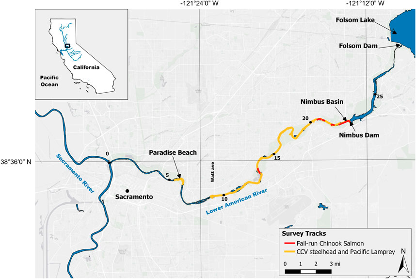
FIGURE 1. Map of the Lower American River in California. Yellow lines represent areas where CCV steelhead and Pacific Lamprey spawning surveys were conducted, and red lines represent areas where fall-run Chinook Salmon spawning surveys were conducted. River miles are represented by black dots with the confluence of the Lower American River and Sacramento River beginning at river mile 0.
Anadromous fish species
Habitat degradation due to the factors described above has adversely impacted several anadromous fish species that occur in the LAR. In California, the presence of impassable dams block an estimated 80% of historical habitat for CCV steelhead distinct population segment (DPS) and all historical spawning habitat for 38% of historical populations (Lindley et al., 2006). As a result, CCV steelhead populations are perilously low and federally listed as threatened (79 FR 20802) under the Endangered Species Act (ESA). CCV steelhead are not listed under the California Endangered Species Act (CESA) but hold a state rank of S2S3 (imperiled/vulnerable). In California, imperiled S2 rank states that a species is at high risk of extirpation due to restricted range, few populations or occurrences, steep declines, severe threats or other factors (California Natural Diversity Database, 2022). Both resident rainbow trout and anadromous steelhead occur in the LAR, and both life history strategies are included in the CCV steelhead DPS. Fall-run Chinook Salmon and Pacific Lamprey also occur on the LAR, are species of special concern for state and federal resource managers, and produce redds during similar time periods that are superficially similar in architecture to CCV steelhead (Gallagher et al., 2007). Therefore, there is potential for unoccupied redd species misidentification.
The three anadromous fish species present in the LAR all build redds in which they lay eggs, but they are differentiated to some extent in terms of spawning timing. In California’s Mediterranean climate, fall-run Chinook Salmon tend to access spawning grounds at rainy season onset, which can vary inter-annually on the order of weeks or even months. However, spawning generally peaks during the months of November and December. Eggs incubate in the gravel and juveniles emerge and out-migrate the following spring. In contrast, CCV steelhead spawn in the winter and early spring, and juveniles may either out-migrate to the ocean or continue to rear in the river for one or more years. There is a less distinct environmental cue that initiates spawning for CCV steelhead and redds have been documented as early as late December (McEwan 2001; Hannon and Deason 2008; Chase 2010). Both salmonid species use hydraulic lift created by tail fanning to mobilize sediments from the redd site. However, redd size is known to vary across salmonids, primarily in relation to body size (Gallagher and Gallagher 2005; Riebe et al., 2014). Fall-run Chinook Salmon are larger, generally resulting in larger redds compared to later spawning CCV steelhead. In contrast, Pacific Lamprey spawning peaks slightly later than CCV steelhead and lamprey may remain in the river for several years as ammocoetes prior to migrating to the ocean and then returning to the river to spawn. Adult Pacific Lamprey move substrate particles primarily by attaching their mouths to rocks and moving individual pieces. Pacific Lamprey also have smaller redds due to smaller body size.
Field methods
Fall-run Chinook Salmon spawning surveys were conducted from 2011 to 2015 and generally occurred every other week from late October to late December, which is when fall-run Chinook Salmon typically spawn in the Central Valley (Williams 2001). These surveys were targeted to assess habitat use following habitat enhancement and were conducted only in gravel augmentation sites at Nimbus Basin, Sailor Bar, Upper Sunrise Side Channel, and Riverbend Park (Figure 1; total coverage varied between 5–8 total rkm, depending on survey year). CCV steelhead spawning surveys were conducted from 2003–2021, with the exception of 2006 and 2008 when surveys were not successful due to high turbidity. Surveys occurred between early January and mid-April and encompassed the entire spawning reach, from Nimbus Basin downstream to Paradise Beach (29 rkm). Pacific Lamprey redds were not explicitly targeted by surveys but were instead observed and measured opportunistically during CCV steelhead spawning surveys. Occasionally, fall-run Chinook Salmon were recorded during CCV steelhead surveys and vice versa.
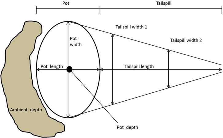
Spawning surveys were conducted either on foot or via rafts/motorized boat by teams of two to four surveying the river from bank to bank, including side channels, visually searching for redds. Surveyors wore polarized sunglasses to improve their ability to see below the water surface. When a redd was observed, a global positioning system (GPS) location and physical measurements were recorded on a Trimble Geoexplorer GPS unit. Redd measurements were based on those used in California coastal spawning surveys (Gallagher 2002). Physical measurements were only taken on redds whose dimensions were not obscured during digging activity by other spawners. Egg pocket length and width were measured along the longest and widest axes (Figure 2). Tailspill length was measured from the back of the pocket to the end of the tailspill. Tailspill width was measured twice, at one-third and two-thirds of total tailspill length, and average width was calculated from these two values. Pocket depth was measured at the redd nose and directly over the egg pocket, and ambient depth was measured upstream from the egg pocket. Depth was recorded from a top-setting velocity rod and depth-averaged velocity was approximated by assuming a logarithmic velocity profile and taking a measurement at 60% of the depth with an electromagnetic Hach FH 950 Flow Meter (Hach manufacturing, Loveland, CO). For depths greater than 0.6 meter (m), two velocity measurements were recorded at 20% and 80% of total depth, and these values were averaged (Hynes 1970). Velocity measurements were taken over a 20-s average and recorded to the nearest 0.01 meter per second (m/s). When a fish was observed associated with a redd, it was identified to species and sex if possible and its length estimated. If visible, surveyors also recorded the presence or absence of an adipose fin. The Nimbus Hatchery has been in operation since 1958 and produces both Chinook Salmon and CCV steelhead. All CCV steelhead produced at the hatchery have their adipose fin clipped to compare hatchery-versus wild-spawned returning adults. Since 2007, 25% of Chinook Salmon from the Nimbus Hatchery have also been clipped as juveniles prior to release.
Spatial data were differentially corrected to increase GPS point accuracy using Trimble Pathfinder Office software (Trimble Navigation, Ltd., Sunnyvale, CA). When redds from two successive surveys were recorded by GPS unit within 5 m of each other, the data were examined in ArcGIS to determine whether these were likely to be the same redd. If both redds were identified as “new, still clear,” it was assumed these dimensions represented a single redd completed over the two survey periods. Therefore, only the second redd and its associated measurements were used in the composite shapefile for the year. For the 2020 and 2021 surveys, this post-processing step resulted in removal of one redd from the raw dataset.
Discriminant function analysis
A DFA model predicts a categorical variable (X) based on known responses (Y). We used a DFA to predict redds to species based on observed values of several continuous variables. Data used to build the predictive model consisted of a sample of observations with known group membership (i.e., fish associated with a redd was identified to species) and several continuous variables that define the physical characteristics or timing of a redd. Model variables were transformed to meet the DFA requirements (i.e., normally distributed data with equal variance). Continuous variables and transformations used in this model included redd depth (no transformation), pot length [natural log(ln)], pot width (ln), pot depth (no transformation), tailspill length (no transformation), river velocity (no transformation), and observation day (no transformation). Observation day was assigned based on the seasonal timing of redd observations, starting at the earliest date on which a redd was recorded and ending on the last recorded date (i.e., October 23–May 2 = 1–190). This is similar to the concept of Julian Day, but reflects the fact that observations recorded at the end of the year (i.e., late December) are more similar to those occurring early in the beginning of the year (i.e., early January), which is not possible if Julian days are used.
DFA analysis was run iteratively from 2016–2021; during each year, any additional “fish on” observations were added each year to improve the model. Analyses were completed using linear DFA in R (R Program Core Team, 2020) using the lda() function in the MASS package (Venables and Ripley 2002). Eigenvalues (trace), which describes the proportion of between class variance explained by linear discriminants (LD1 and LD2), was also estimated using lda (). Cohen’s Kappa, which measures percent agreement of species identity, was estimated using the Cohen. kappa() function in the psych package (Revelle 2016). A scatter plot was generated to visualize inter-species differences and variation in the linear discriminants (LD1 and LD2).
Comparisons of redd metrics across species were made using an Analysis of Variance (ANOVA) and pairwise comparisons between species were made using a Tukey post-hoc test, using a significance threshold of p = 0.01. All analyses were run using the R package car (Fox and Weisberg 2019).
Historical survey species identification comparisons
The 2021 iteration of the DFA model was applied to historical data collected between 2003–2015 in which no fish were observed but redd measurements were recorded and species identification was assigned based on professional opinion. To determine the similarity in outcome between the two approaches, professional opinion identification was compared to the model’s predicted species identification and proportion agreement in identification between the methods was calculated for each survey season (Oct–May) by summing the number of disagreements for a given year and dividing that number by the total redds observed that year.
Results
A total of 1,597 redds were documented in the LAR between 2003 and 2021 (Table 1). Of the redds observed, 1,104 were unoccupied, 179 were occupied by fall-run Chinook Salmon, 46 by Pacific Lamprey, and 268 by CCV steelhead. Fall-run Chinook Salmon spawning surveys (2011–2016) were conducted from late October through late December; CCV steelhead spawning surveys (2003–2021) were conducted from early January through April. During the period when the surveys were conducted, flows ranged from a low of 13.6 cubic meters per second (cms) in 2015–2016 to a high of 2,333.3 cms in 2017 (Table 1).
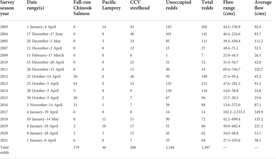
TABLE 1. Summary of redds observed by year and species, and unoccupied redds. The data range when each year of surveys was conducted and the average and range of flows during that timeframe is also provided. Insufficient data were available for 2006 and no surveys were conducted in 2008.
Discriminant function analysis
The DFA model included the following predictors: Seasonal Timing, Redd Depth, Velocity, Pot Length, Pot Width, Pot Depth, and Tailspill Length. Pot Length and Pot Width were natural log transformed to meet model assumptions. In 2016 and 2017, the model only included data from CCV steelhead and fall-run Chinook Salmon; in 2018, Pacific Lamprey data were added to the model after it was recognized that their spawning time overlapped substantially with CCV steelhead. Redds were excluded from analysis if they lacked key variables that were necessary to build the model. The final (2021) iteration of the discriminant function was built using 183 fall-run Chinook Salmon redds, 268 CCV steelhead redds, and 46 Pacific Lamprey redds with positively identified fish observations, collected between 2003 and 2021. Redds observed occupied by fall-run Chinook Salmon were recorded between 23 October and 4 February, with the peak number of redds recorded on 23 November (SD = 18 days). Redds observed by occupied by CCV steelhead were observed between 29 December and 19 April, with a peak number of redds observed on 10 February (SD = 20 days). Redds observed occupied by Pacific Lamprey were recorded between 9 January and 18 May, with a peak number of redds observed on 28 March (SD = 24 days) (Figure 3). Differences in seasonal spawning timing were significantly different across all species (all Tukey p < 0.001).
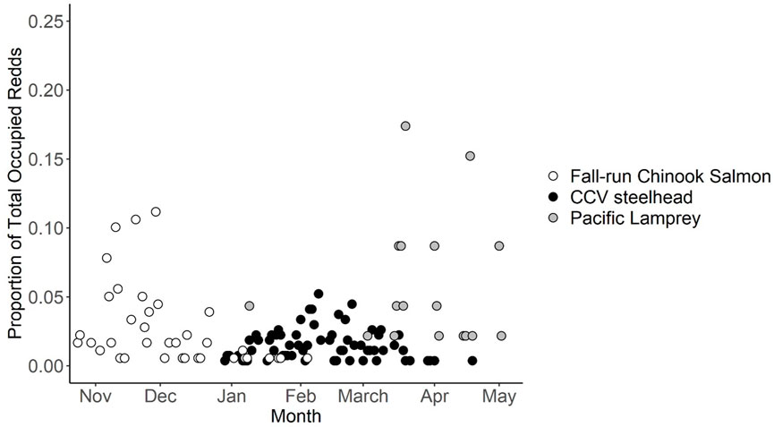
FIGURE 3. Temporal distribution of proportion of redds observed occupied by either Fall-run Chinook Salmon, CCV steelhead and Pacific Lamprey between 2003 and 2021.
The other factors included in the DFA model are summarized across the three species in Figure 4. There was variation across species in most of the factors, except for Pot Depth which did not differ significantly in any pairwise comparisons (Tukey post-hoc test, all p > 0.01). Fall-run Chinook Salmon spawned in shallower depths compared to the other two species, Pacific Lamprey differed from the salmonid species in velocity and pot dimensions, and all three species had distinct average tailspill lengths.
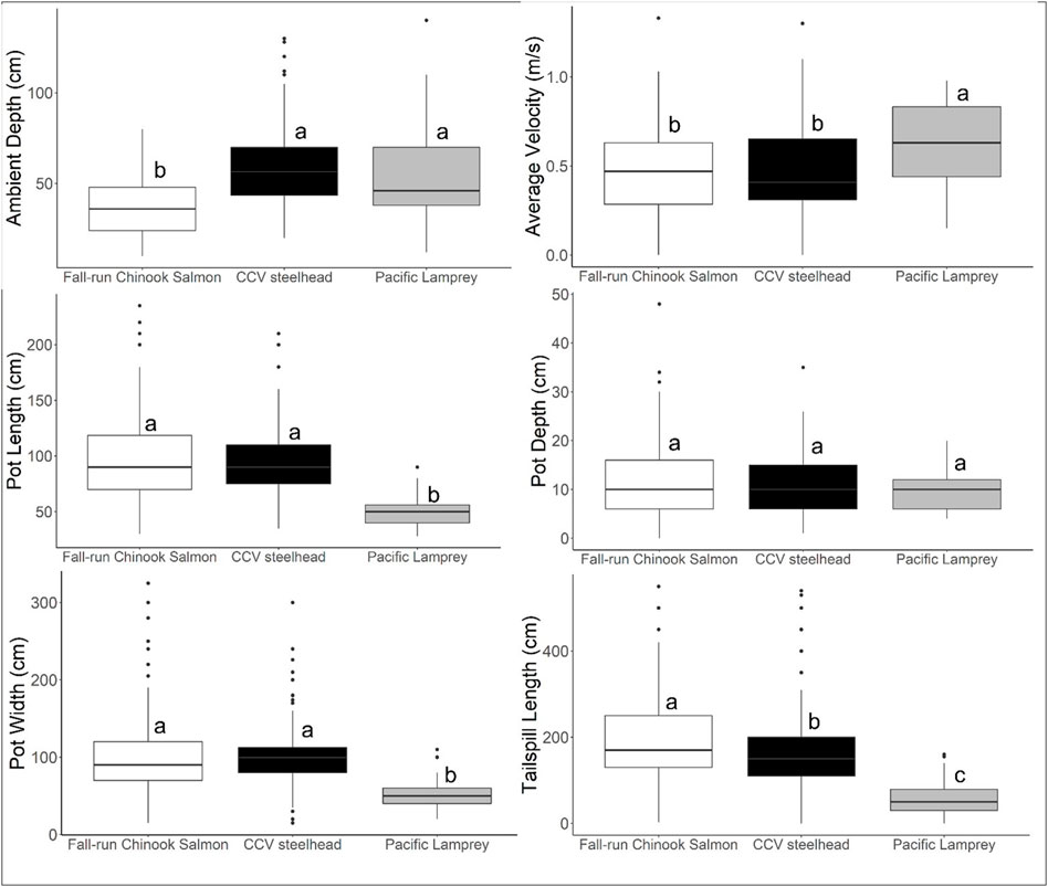
FIGURE 4. Comparison across species of redd metrics used for developing DFA. Within each redd metric, box plots with different letters indicate significant pairwise differences using a Tukey post-hoc test, using a significance threshold of p = 0.01.
The eigenvalue (trace) for the final (2021) iteration of the model was 0.95 for LD1 and 0.05 for LD2. This indicates that 95% of the between-group variance exists along the first discriminant axis, which is heavily weighted by velocity (Table 2). Overall, model accuracy was 95.7% and the Cohen’s Kappa was predicted as 0.94, indicating high model agreement for species categorization.
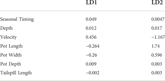
TABLE 2. Coefficients from the 2021 DFA model, which show the loading of each covariate on the discriminants.
Velocity was the dominant model covariate and was weighted heavily in both LD1 and LD2 (0.456 and −1.167, respectively). Seasonal timing was the second highest coefficient in LD1 (0.049) but was low in LD2 (0.005). Pot length was the highest coefficient (1.744) in LD2 but was relatively low in LD1 (−0.264). These three factors strongly differentiated Pacific Lamprey from the two salmonid species (Table 2). The other variable coefficients were small for both LD1 and LD2, indicating that they had a relatively small impact on species prediction (Table 2). A scatter plot visualizing LD1 and LD2 variation across species of redd metrics is provided in Figure 5.
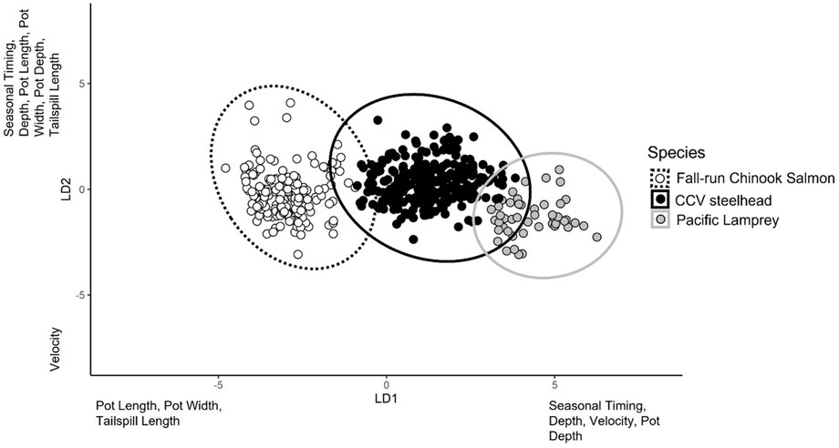
FIGURE 5. Scatter plot of linear discriminant analysis scores LD1 and LD2 describing variation across species of redds metrics.
Accuracy of the DFA model in predicting redd species using historical data from known redd identity between 2016–2021 is provided. Overall, the model had over 96% accuracy for both salmonid species for all 6 years in which it was applied. Fall-run Chinook Salmon accuracy decreased slightly from 99% accuracy in 2016 through 2019 to 97% accuracy in 2020 and 96% accuracy in 2021 when additional later spawning fall-run Chinook Salmon observations were added to the model. The model had relatively high CCV steelhead accuracy throughout the 5 years, ranging from 96%–99% (Figure 6).
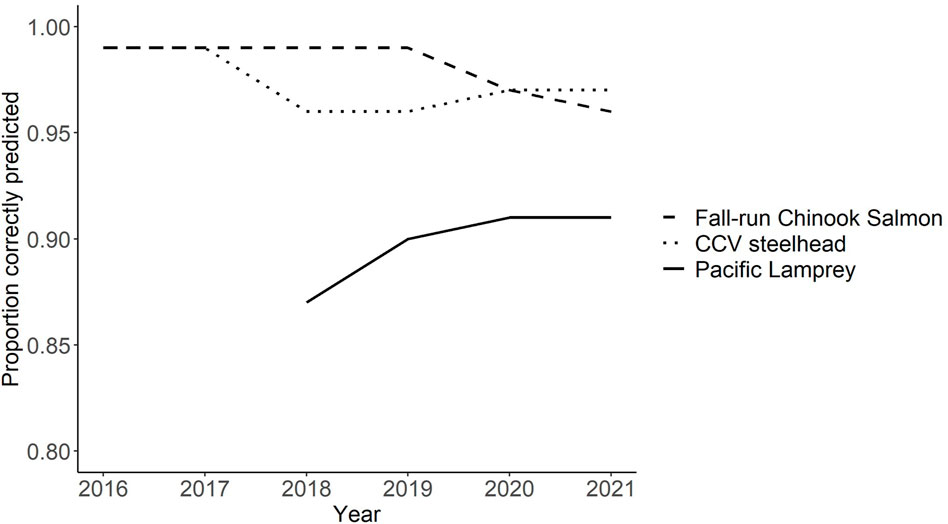
FIGURE 6. Proportion of redds correctly identified between species using the discriminant function analysis model between 2016 and 2021.
In 2021, the model correctly predicted 171 of the 179 (95.5%) total fall-run Chinook Salmon redds; eight incorrect assignments were predicted to be CCV steelhead (Table 3). Forty-two of the 46 Pacific Lamprey were correctly predicted (91.3%), and the remaining four were predicted to be CCV steelhead. A total of 259 of the 268 CCV steelhead redds were correctly assigned (96.6%). Of the nine CCV steelhead redds that were incorrectly assigned, two of these were predicted to be fall-run Chinook Salmon and seven were predicted to be Pacific Lamprey redds. Most incorrect assignments across species were caused by fish in the population with atypical spawning timing or redd dimensions. For example, fall-run Chinook Salmon that were predicted to be CCV steelhead had an average spawning date of 13 January, when the overall population had a peak number of redds observed on 23 November. Pacific Lamprey redds that were predicted to be CCV steelhead had a spawning date of 9 January (population peak number redds observed on 28 March) or had a tailspill lengths and/or pot widths greater than 100 cm (mean = 56.8 cm and 52.7 cm, respectively). Several CCV steelhead that were incorrectly predicted to be Pacific Lamprey had pot lengths between 50 cm and 60 cm (mean = 95 cm).

TABLE 3. Predicted (column) and actual (row) species designations in discriminant function analysis. “Total” column indicates predicted number of redds, and “Total” row indicates actual number of redds for each species.
Historical surveys species identification comparisons
Prior to the development of the DFA model in 2016 to predict redd species identity, 833 unoccupied redds were observed and identified using professional opinion between 2003 and 2015. To compare the species identifications using professional opinion with that predicted by the DFA model, we applied the 2021 iteration of the model to this dataset (Table 4).
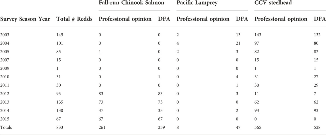
TABLE 4. Comparison between redd identification based on professional opinion versus the discriminant function analysis.
During the first few years in which redd surveys were conducted, a relatively large proportion of redds visually identified as CCV steelhead were categorized by the DFA as Pacific Lamprey redds (7.7% in 2003, 17.5% in 2004; Figure 7). Disagreements between identifications based on professional opinion and the DFA prediction were lower in future years, but there were at least a few disagreements between the two methods in 2005, 2010, 2011, 2012, and 2014, primarily with redds identified visually as CCV steelhead being identified as either fall-run Chinook Salmon or Pacific Lamprey by the model.
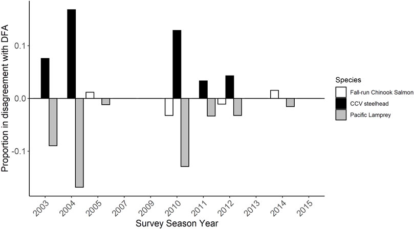
FIGURE 7. The proportion of redd species identifications based on professional opinion that differed from that obtained using the 2021 DFA model. The y axis represents the number of disagreements in redd identification between professional opinion and the DFA prediction divided by the total redds observed that year.
Another application of the DFA is retro-actively identifying historically unidentified redds. In the LAR dataset, this approach allowed a predictive identification of a total of five Pacific Lamprey redds in 2004, one Pacific Lamprey and two CCV steelhead redds in 2005, and seven CCV steelhead redds in 2015 that were previously excluded from total redd counts and any subsequent annual population estimates derived from the data.
Discussion
Resource partitioning in degraded systems
Habitat is a major dimension of resource partitioning in stream fishes and may arise from each species’ genetically determined tendency to select different microhabitats independent of other species (Schoener 1974). Quantifying differential habitat selection (also known as niche partitioning) is a common approach used by ecologists to understand ecological segregation between closely-related but spatially overlapping species (e.g., Morris 2003; Nicholls and Racey 2006; Pita et al., 2011), and there is growing evidence that habitat selection is a scale-dependent process (Mayor et al., 2009). However, in a dynamic or highly degraded environment a high degree of habitat specialization may not be a successful ecological trait for species persistence, and individuals within a population may demonstrate plastic and opportunistic habitat use (Schwemmer et al., 2008; Moss et al., 2016). This flexibility can make it difficult to quantify habitat preference by guild, especially when individuals are not physically present within an observed territory. However, our results demonstrate that if relevant habitat metrics are incorporated, a predictive model can be a powerful tool to improve the objectivity and accuracy of redd identification of three co-occurring anadromous fish species. This has implications for optimizing restoration practices and water management decisions in a highly impacted system with multiple species of concern.
Niche differentiation across species in the LAR
While all three LAR native anadromous fish species tend to spawn in gravel rich habitats predominantly associated with pool tail-outs and low gradient riffles, we found strong evidence for niche differentiation within these habitat patches which may result from species-specific distinctions in spawning timing, body size, and how each species perceives and uses preferred habitats including redd construction mechanisms. Fall-run Chinook Salmon timing coincided with the onset of the rainy season (November–December, while CCV steelhead spawned peak spawning occurred in February-March and Pacific Lamprey spawned primarily in March and April. Redd size varied across species, associated with body size and method of redd construction, with Chinook Salmon producing the largest redds and Pacific Lamprey producing the smallest redds. These inter-species distinctions resulted in the DFA model being driven by three variables: water velocity, seasonal timing, and redd (pot) size.
Seasonal timing was historically the primary factor used for professional opinion identification between fall-run Chinook Salmon, CCV steelhead and Pacific Lamprey. However, there is temporal overlap during the spawning period for the two salmonid species and lamprey, particularly in heavily managed systems where flow is not necessarily correlated with precipitation or during years with delayed rainy season initiation. A trend towards later fall-run Chinook Salmon spawning timing in particular has been observed in recent years on the LAR, possibly due to a combination of prolonged drought, stressful water temperatures in the early fall, and flow and hatchery management practices (CDFW unpublished data; Quinn et al., 2002; Austin et al., 2021). Flow management practices on the LAR include operating Folsom and Nimbus facilities to avoid high flows during fall run Chinook Salmon spawning. This operational decision is meant to prevent spawners from building redds at higher flows which could cause future redd dewatering if low winter precipitation results in flow reductions to conserve reservoir storage. This may also explain the shallower spawning depths observed in the LAR for fall-run Chinook Salmon compared to CCV steelhead and Pacific Lamprey. Despite the temporal overlap, because the three species differed in hydraulic preferences and redd architecture, model results enabled identification of historically unidentified or potentially mis-identified redds, enhancing data quality and subsequent population estimates.
Despite the overall tendency for habitat segregation, fall-run Chinook Salmon, CCV steelhead and Pacific Lamprey showed considerable overlap in habitat preferences within the highly managed and marginalized habitat of the LAR. For example, pot depth was similar across all three species, ambient depth was similar for CCV steelhead and Pacific Lamprey, and pot width and length were similar for fall-run Chinook Salmon and CCV steelhead. There are certain essential habitat characteristics for substrate spawners, including material that can be mobilized but not scour and cool, oxygenated water carried to and metabolic wastes removed from incubating embryos (Merz et al., 2019; Bilski et al., 2022). While spawning habitat restoration practices such as gravel augmentation can provide core habitat for a range of species provided that water quality is suitable, inter-specific differences must also be taken into account when selecting augmentation features and locations. These differences are also important for developing species-specific habitat suitability predictions for restoration designs that integrate depth and velocity conditions under varying flows (Wheaton et al., 2004). The DFA model presented here and the data used to generate the model can help restoration practitioners identify key habitat requirements that may support multiple target species. However, future work is needed and additional metrics such as substrate size and distance from impassable dam could be incorporated into future model iterations.
The ability to incorporate physical and temporal variables to predict species spawning sites from a guild of three species with a range of management implications offers a powerful management tool and highlights the value of data collection quality, even on perceived, less valuable species. Fall-run Chinook Salmon have the highest commercial economic value, CCV steelhead is a highly-prized sport fish and focus of federal protection and are often competitive for limited LAR water resources (McEwan, 2001; Williams 2001). In contrast, Pacific Lamprey are harvested primarily for bait (sturgeon fishing), receiving relatively little management attention, even though they are an important ecological component within the CCV (Close et al., 2002). Given the temporal and spatial overlap in spawning with these other species. Limiting data collection to salmonid species reduces accuracy of CCV steelhead redd identification and, subsequently, population estimates.
Iterative model refinement
Our results also demonstrate the utility of iteratively updating and refining models as additional data become available. Comparison with data from occupied redds demonstrated that the model had a high degree of accuracy and model robustness increased across several iterative incorporations of new data, with >96% accuracy for the two salmonids and >91% for Pacific Lamprey. This DFA modeling approach has the potential to enhance survey integrity and accuracy of where species identification for redd surveys or other surveys that involve challenging species identification is based on biometrics or physical habitat metrics for which a reference dataset is available. With subsequent years of data collection, particularly on Pacific Lamprey redds, the model accuracy in predicting species identity is expected to further increase. Increased objectivity in species identification across survey years and geographical regions will ultimately support more informed management decisions.
Limitations and future research
Substrate size is also known to be an important factor in female spawning site selection and tends to scale with females body size, with female salmonids typically spawning in gravel substrates with a median diameter up to about 10% of their body length (1.3–2.6 cm) (Bjornn and Reiser 1991; Kondolf and Wolman 1993). Zeug et al. (2013) found that grain size had a strong influence on both fall-run Chinook Salmon and CCV steelhead site selection as well as the size and shape of completed redds. While average substrate size was often recorded in field measurements, ultimately these data could not be incorporated into our model because we identified dataset irregularities indicating this metric was not standardized across surveys. No clear protocol was available for collecting substrate size information during redd surveys as it was for the other redd metrics, limiting the data’s utility. Because of its clear relationship with female site selection and body size, incorporating additional field metrics to record substrate size information, such as standardized photographs, would allow substrate to be incorporated into future iterations of this model. Obtaining high quality data for this habitat metric, in particular, has strong implications for habitat restoration in a sediment-starved river, where the stream bed tends to armor over time and the use of overly coarse sediment for gravel augmentation may exclude smaller-bodied species such as CCV steelhead and Pacific Lamprey (Zeug et al., 2013). Standardized sediment data could inform design of gravel augmentation actions intended to target CCV steelhead populations by providing a distribution of substrate size preferences for this species.
Management implications
Inaccurate species identification can impact subsequent population estimates, management decisions, and restoration approaches. CCV Steelhead survey data has been used to develop population estimates for this federally threatened species on the LAR for the past two decades. During this time, annual redd counts have ranged from 12–314, with subsequent population estimates between 45–504 reproducing adults. With such a low number of individuals in the system, even a few misidentified redds could significantly reduce the accuracy of the resulting population estimate. In addition to informing resource managers about annual salmon population size, physical redd measurements from both CCV steelhead and fall-run Chinook Salmon on the LAR has been used to inform restoration designs and determine site utilization on recent gravel augmentation projects (Zeug et al., 2013; Merz et al., 2019; cbec, personal communication). If redd species identification is incorrect, this could lead to a misrepresentation of species’ spatial distribution or preferred physical parameters (e.g., substrate size, depth, and velocity) for target species, subsequently reducing restoration effectiveness. The modeling approach described here can increase data accuracy and objectivity, providing higher quality information to support decision making.
On the American River, as in all other major CCV rivers, most historic salmonid and presumably Pacific Lamprey spawning habitat is impounded behind impassible dams, greatly reducing channel types and gradients available to these three species (Yoshiyama et al., 1998). In addition, the region has experienced prolonged periods of drought in recent years that have resulted in low streamflow and stressful temperature conditions, particularly during the early fall. As mentioned above, this has resulted in a trend towards later spawning by fall-run Chinook Salmon and subsequently greater temporal niche overlap between this species and CCV steelhead. Gabor et al. (2001) have reported that mammals have documented higher inter-specific overlap during harsh environmental conditions, such as droughts. The degraded condition of the LAR and other rivers throughout the CCV may force fish species to utilize habitats outside their optimal range, which could obscure our ability to detect niche differentiation across species (Gaines et al., 2000; Kozlowski et al., 2012; Huber and Carlson 2020). However, even in the highly impacted LAR and with a relatively limited dataset, it was possible to successfully classify redds to species using relevant habitat metrics.
Conclusion
By detecting niche segregation between species, modeling like that described here can improve understanding of the functional scales of habitat fragmentation, thereby providing information on critical thresholds regarding the spatial extent and distribution of resources for target species (Thompson and McGarigal, 2002). This approach can allow resource managers to target habitat restoration design for particular species, or generate designs that provide habitat for all three species, and track species management success where multiple species have overlapping but distinct habitat requirements.
Data availability statement
The raw data supporting the conclusion of this article will be made available by the authors, without undue reservation.
Ethics statement
Ethical review and approval was not required for the animal study because the data was collected using observation and measurement of anadromous fish redds in the wild. No fish were physically handled or harassed during sampling.
Author contributions
KS—Conceptualization, Project administration, Funding acquisition, Supervision, Methodology, Data curation, Formal analysis, Writing, and Revision. JS: Investigation, Data curation, Formal analysis, Visualization, Writing, and Revision. JM: Conceptualization, Funding acquisition, Supervision, Writing, and Revision.
Funding
Sacramento Water Forum and Bureau of Reclamation (Grant #140R2020C0006) provided funding for data collection and analysis for this manuscript.
Acknowledgments
Sacramento Water Forum staff provided input on the draft manuscript. California Department of Fish and Wildlife shared unpublished data to provide context for the temporal distribution of Chinook Salmon in the LAR. Bureau of Reclamation staff including John Hannon, Jessica Andreaux, and Spencer Marshall provided feedback on the model structure and components. Numerous Bureau of Reclamation and Cramer Fish Sciences field staff collected the data used in the analysis.
Conflict of interest
The authors declare that the research was conducted in the absence of any commercial or financial relationships that could be construed as a potential conflict of interest.
Publisher’s note
All claims expressed in this article are solely those of the authors and do not necessarily represent those of their affiliated organizations, or those of the publisher, the editors and the reviewers. Any product that may be evaluated in this article, or claim that may be made by its manufacturer, is not guaranteed or endorsed by the publisher.
References
Adams, P. B., Boydstun, L. B., Gallagher, S. P., Lacy, M. K., McDonald, T., and Shaffer, K. E. (2011). Fish bull 180. California coastal salmonid population monitoring: Strategy, design, and methods. San Diego, CA: California Department of Fish and Game.
Austin, C. S., Essington, T. E., and Quinn, T. P. (2021). In a warming river, natural-origin Chinook salmon spawn later but hatchery-origin conspecifics do not. Can. J. Fish. Aquat. Sci. 78 (1), 68–77. doi:10.1139/cjfas-2020-0060
Austin, H., Scoles, D., and Abell, A. J. (1999). Morphometric separation of annual cohorts within mid-atlantic bluefish, pomatomus saltatrix, using discriminant function analysis. VIMS Articles. 585. Accessed at: https://scholarworks.wm.edu/vimsarticles/585/.
Barahoei, H., Madjdzadeh, S. M., and Mehrparvar, M. (2011). Morphometric differentiation of five biotypes of Lysiphlebus fabarum (Marshall)(Hymenoptera: Braconidae: Aphidiinae) in Iran. Zootaxa 2745 (1), 43–52. doi:10.11646/zootaxa.2745.1.3
Barbarossa, V., Schmitt, R. J. P., Huijbregts, M. A. J., Zarfl, C., King, H., and Schipper, A. M. (2020). Impacts of current and future large dams on the geographic range connectivity of freshwater fish worldwide. Proc. Natl. Acad. Sci. U. S. A. 117, 3648–3655. doi:10.1073/pnas.1912776117
Beakes, M. P., Moore, J. W., Retford, N., Brown, R., Merz, J. E., and Sogard, S. M. (2014). Evaluating statistical approaches to quantifying juvenile Chinook salmon habitat in a regulated California river. River Res. Appl. 30 (2), 180–191. doi:10.1002/rra.2632
Bilski, R. L., Wheaton, J. M., and Merz, J. E. (2022). Effects of in-channel structure on Chinook salmon spawning habitat and embryo production. Water 14 (1), 83. doi:10.3390/w14010083
Bjornn, T. C., and Reiser, D. W. (1991). Habitat requirements of salmonids in streams. Am. Fish. Soc. Special Publ. 19 (837), 138.
Brown, M. T., and Wicker, L. R. (2000). “Discriminant analysis,” in Handbook of applied multivariate statistics and mathematical modeling (Cambridge, MA: Academic Press), 209–235.
Burner, C. J. (1951). Characteristics of spawning nests of columbia river salmon. U.S. Fish and Wildlife service. Fish. Bull. 61 (52), 97–110.
California Natural Diversity Database (CNDDB) (2022). Special animals list. Sacramento, CA: California Department of Fish and Wildlife (Accessed July, 2022).
Chase, R. (2010). Lower American River steelhead (Oncorhynchus mykiss) spawning surveys–2010. Sacramento, CA: Department of the Interior, US Bureau of Reclamation, 17.
Close, D. A., Fitzpatrick, M. S., and Li, H. W. (2002). The ecological and cultural importance of a species at risk of extinction, Pacific Lamprey. Fisheries 27 (7), 19–25. doi:10.1577/1548-8446(2002)027<0019:teacio>2.0.co;2
Desai, M., Husted, A., Fry, C., Downs, C. T., and O’Brien, G. C. (2019). Spatial shifts and habitat partitioning of ichthyofauna within the middle–lower region of the Pungwe Basin, Mozambique. J. Freshw. Ecol. 34 (1), 685–702. doi:10.1080/02705060.2019.1673221
Falke, J. A., Dunham, J. B., Jordan, C. E., McNyset, K. M., and Reeves, G. H. (2013). Spatial ecological processes and local factors predict the distribution and abundance of spawning by steelhead (Oncorhynchus mykiss) across a complex riverscape. PLoS One 8 (11), e79232. doi:10.1371/journal.pone.0079232
Fox, J., and Weisberg, S. (2019). An R companion to applied regression. Third edition. Los Angeles, CA: SAGE Publishing.
Fukushima, M., and Smoker, W. W. (1998). Spawning habitat segregation of sympatric sockeye and pink salmon. Trans. Am. Fish. Soc. 127 (2), 253–260. doi:10.1577/1548-8659(1998)127<0253:shsoss>2.0.co;2
Gabor, T. M., Hellgren, E. C., and Silvy, N. J. (2001). Multi-scale habitat partitioning in sympatric suiforms. J. Wildl. Manag. 65, 99–110. doi:10.2307/3803281
Gaines, K. F., Bryan, A. L., and Dixon, P. M. (2000). The effects of drought on foraging habitat selection of breeding Wood Storks in coastal Georgia. Waterbirds, 64–73.
Gallagher, S. P., Adams, P. B., Wright, D. W., and Collins, B. W. (2010). Performance of spawner survey techniques at low abundance levels. North Am. J. Fish. Manag. 30 (5), 1086–1097. doi:10.1577/m09-204.1
Gallagher, S. P., and Gallagher, C. M. (2005). Discrimination of Chinook salmon, coho salmon, and steelhead redds and evaluation of the use of redd data for estimating escapement in several unregulated streams in northern California. North Am. J. Fish. Manag. 25 (1), 284–300. doi:10.1577/m04-016.1
Gallagher, S. P., Hahn, P. K., and Johnson, D. H. (2007). Salmonid field protocols handbook: Techniques for assessing status and trends in salmon and trout populations. Bethesda, Maryland: American Fisheries Society, 197–234.Redd counts.
Gallagher, S. P. (2002). Salmonid spawning survey protocols for 2002–2003. Fort Bragg, CA: California State Department of Fish and Game, 14.
Hannon, J. (2013). American River Steelhead (Oncorhynchus mykiss) Spawning-2013 with comparisons to prior years. Sacramento, CA: US Bureau of Reclamation, 32.
Hannon, J., and Deason, B. (2008). American river steelhead (Oncorhynchus mykiss) spawning 2001–2007. Mid-Pacific Region: US Department of the Interior, Bureau of Reclamation.
Hayden, T. A., Binder, R. B., Holbrook, C. M., Vandergoot, C. S., Fielder, D. G., Cooke, S. J., et al. (2018). Spawning site fidelity and apparent annual survival of walleye (Sander vitreus) differ between a Lake Huron and Lake Erie tributary. Ecol. Freshw. Fish. 27, 339–349. doi:10.1111/eff.12350
Herring, G., Ackerman, J. T., Eagles-Smith, C. A., and Takekawa, J. Y. (2010). Sexing California gulls using morphometrics and discriminant function analysis. Waterbirds 33 (1), 79–85. doi:10.1675/063.033.0109
Huber, E. R., and Carlson, S. M. (2020). Environmental correlates of fine-scale juvenile steelhead trout (Oncorhynchus mykiss) habitat use and movement patterns in an intermittent estuary during drought. Environ. Biol. Fishes 103, 509–529. doi:10.1007/s10641-020-00971-y
Hynes, H. B. N. (1970). The ecology of flowing waters in relation to management. J. Water Pollut. Control Fed. 42, 418–424.
James, L. A. (1997). Channel incision on the lower American River, California, from streamflow gage records. Water Resour. Res. 33 (3), 485–490. doi:10.1029/96wr03685
Kondolf, G. M., Boulton, A. J., O'Daniel, S., Poole, G. C., Rahel, F. J., Stanley, E. H., et al. (2006). Process-based ecological river restoration: Visualizing three731 dimensional connectivity and dynamic vectors to recover lost linkages. Ecol. Soc. 11 (2), 1–16. ISSN 1708-3087.
Kondolf, G. M., and Wolman, M. G. (1993). The sizes of salmonid spawning gravels. Water Resour. Res. 29 (7), 2275–2285. doi:10.1029/93wr00402
Kozlowski, A. J., Gese, E. M., and Arjo, W. M. (2012). Effects of intraguild predation: Evaluating resource competition between two canid species with apparent niche separation. Int. J. Ecol. 2012, 1–12. doi:10.1155/2012/629246
Lane, C. R., Leibowitz, S. G., Autrey, B. C., LeDuc, S. D., and Alexander, L. C. (2018). Hydrological, physical, and chemical functions and connectivity of non-floodplain wetlands to downstream waters: A review. J. Am. Water Resour. Assoc. 54 (2), 346–371. doi:10.1111/1752-1688.12633
Liermann, C. R., Nilsson, C., Robertson, J., and Ng, R. Y. (2012). Implications of dam obstruction for global freshwater fish diversity. Bioscience 62, 539–548. doi:10.1525/bio.2012.62.6.5
Lindley, S. T., Schick, R. S., Agrawal, A., Goslin, M., Pearson, T. E., Mora, E., et al. (2006). Historical population structure of Central Valley steelhead and its alteration by dams. San Franc. Estuary Watershed Sci. 4 (1). doi:10.15447/sfews.2006v4iss1art3
Mayor, S. J., Schneider, D. C., Schaefer, J. A., and Mahoney, S. P. (2009). Habitat selection at multiple scales. Ecoscience 16 (2), 238–247. doi:10.2980/16-2-3238
McElhany, P., Rucklelshaus, M. H., Ford, M. J., Wainwright, T. C., and Bjorkstedt, E. P. (2000). Viable salmonid populations and the recovery of evolutionarily significant units. Seattle, WA: NOAA Technical Memorandum NMFS-NWFSC-42.
McManamay, R. A., Orth, D. J., Dolloff, C. A., and Cantrell, M. A. (2010). Gravel addition as a habitat restoration technique for tailwaters. North Am. J. Fish. Manag. 30 (5), 1238–1257. doi:10.1577/m10-007.1
McMillan, J. R., Pess, G. R., Liermann, M., Morley, S. A., McHenry, M. L., Campbell, L. A., et al. (2015). Using redd attributes, fry density, and otolith microchemistry to distinguish the presence of steelhead and rainbow trout in the elwha river dam removal project. N. Am. J. Fish. Manag. 35, 1019–1033. doi:10.1080/02755947.2015.1074965
Meffe, G. K. (1986). Conservation genetics and the management of endangered fishes. Fisheries 11 (1), 14–23. doi:10.1577/1548-8446(1986)011<0014:cgatmo>2.0.co;2
Merz, J., Caldwell, L., Beakes, M., Hammersmark, C., and Sellheim, K. (2019). Balancing competing life-stage requirements in salmon habitat rehabilitation: Between a rock and a hard place. Restor. Ecol. 27 (3), 661–671. doi:10.1111/rec.12900
Merz, J. E., Workman, M., Threloff, D., and Cavallo, B. (2013). Salmon lifecycle considerations to guide stream management: examples from California's Central Valley. San Francisco Estuary Watershed Sci. 11 (2).
Merz, J. E., and Vanicek, C. D. (1996). Comparative feeding habits of juvenile Chinook salmon, steelhead, and Sacramento squawfish in the lower American River, California. Calif. Fish Game 82 (4), 149–159.
Montgomery, D. R., Buffington, J. M., Peterson, N. P., Schuett-Hames, D., and Quinn, T. P. (1996). Stream-bed scour, egg burial depths, and the influence of salmonid spawning on bed surface mobility and embryo survival. Can. J. Fish. Aquat. Sci. 53 (5), 1061–1070. doi:10.1139/f96-028
Morris, D. W. (2003). Toward an ecological synthesis: A case for habitat selection. Oecologia 136 (1), 1–13. doi:10.1007/s00442-003-1241-4
Moss, W. E., Alldredge, M. W., Logan, K. A., and Pauli, J. N. (2016). Human expansion precipitates niche expansion for an opportunistic apex predator (Puma concolor). Sci. Rep. 6 (1), 39639–39645. doi:10.1038/srep39639
Nicholls, B., and Racey, P. A. (2006). Contrasting home-range size and spatial partitioning in cryptic and sympatric pipistrelle bats. Behav. Ecol. Sociobiol. 61 (1), 131–142. doi:10.1007/s00265-006-0244-7
Oregon Department of Fish and Wildlife (ODFW) (2016). Salmon spawning survey procedures manual. Oregon adult salmonid inventory and sampling (OASIS) project. Corvallis, OR: Oregon Department of Fish and Wildlife, 104.
Pita, R., Mira, A., and Beja, P. (2011). Assessing habitat differentiation between coexisting species: The role of spatial scale. Acta Oecol. 37 (2), 124–132. doi:10.1016/j.actao.2011.01.006
Quinn, T. P., Peterson, J. A., Gallucci, V. F., Hershberger, W. K., and Brannon, E. L. (2002). Artificial selection and environmental change: Countervailing factors affecting the timing of spawning by coho and Chinook salmon. Trans. Am. Fish. Soc. 131 (4), 591–598. doi:10.1577/1548-8659(2002)131<0591:asaecc>2.0.co;2
R Program Core Team (2020). R: A language and environment for statistical computing. Vienna, Austria: The R Foundation.
Revelle, W. (2016). How to: Use the psych package for factor analysis and data reduction. Evanston, IL: Northwestern University, Department of Psychology.
Riebe, C. S., Sklar, L. S., Overstreet, B. T., and Wooster, J. K. (2014). Optimal reproduction in salmon spawning substrates linked to grain size and fish length. Water Resour. Res. 50, 898–918. doi:10.1002/2013WR014231
Schoener, T. W. (1974). Resource Partitioning in Ecological Communities: Research on how similar species divide resources helps reveal the natural regulation of species diversity. Science 185 (4145), 27–39. doi:10.1126/science.185.4145.27
Schwemmer, P., Garthe, S., and Mundry, R. (2008). Area utilization of gulls in a coastal farmland landscape: Habitat mosaic supports niche segregation of opportunistic species. Landsc. Ecol. 23 (3), 355–367. doi:10.1007/s10980-008-9194-y
Sellheim, K. L., Watry, C. B., Rook, B., Zeug, S. C., Hannon, J., Zimmerman, J., et al. (2016). Juvenile salmonid utilization of floodplain rearing habitat after gravel augmentation in a regulated river. River Res. Appl. 32 (4), 610–621. doi:10.1002/rra.2876
Staentzel, C., Kondolf, G. M., Schmitt, L., Combroux, I., Barillier, A., and Beisel, J. N. (2020). Restoring fluvial forms and processes by gravel augmentation or bank erosion below dams: A systematic review of ecological responses. Sci. Total Environ. 706, 135743. doi:10.1016/j.scitotenv.2019.135743
Stewart, I. J., Carlson, S. M., Boatright, C. P., Buck, G. B., and Quinn, T. P. (2004). Site fidelity of spawning sockeye salmon (Oncorhynchus nerka) in the presence and absence of olfactory cues. Ecol. Freshw. Fish. 13, 104–110. doi:10.1111/j.1600-0633.2004.00044.x
Susac, G. L., and Jacobs, S. E. (2002). Assessment of the Nestucca and Alsea rivers winter steelhead, 2002. Portland, Oregon: Oregon Department of Fish and Wildlife, 18pp.
Taylor, J. J., Rytwinski, T., Bennett, J. R., Smokorowski, K. E., Lapointe, N. W. R., Janusz, R., et al. (2019). The effectiveness of spawning habitat creation or enhancement for substrate-spawning temperate fish: A systematic review. Environ. Evid. 8, 19–31. doi:10.1186/s13750-019-0162-6
Thompson, C. M., and McGarigal, K. (2002). The influence of research scale on bald eagle habitat selection along the lower Hudson River, New York (USA). Landsc. Ecol. 17 (6), 569–586. doi:10.1023/a:1021501231182
Venables, W. N., and Ripley, B. D. (2002). Modern applied statistics with S. Fourth Edition. New York: Springer. ISBN 0-387-95457-0.
Wagner, H. H. (1969). Effect of stocking location of juvenile steelhead trout, Salmo gairdnerii, on adult catch. Trans. Am. Fish. Soc. 98, 27–34. doi:10.1577/1548-8659(1969)98[27:eosloj]2.0.co;2
Wheaton, J., Pasternack, G., and Merz, J. (2004). “Use of habitat heterogeneity in salmonid spawning habitat rehabilitation design,” in Fifth international symposium on ecohydraulics: Aquatic habitats: Analysis & restoration. Editors D. Garcia, and P. Martinez (Madrid, Spain: IAHR-AIRH), 791–796.
White, J. W., and Ruttenberg, B. I. (2007). Discriminant function analysis in marine ecology: Some oversights and their solutions. Mar. Ecol. Prog. Ser. 329, 301–305. doi:10.3354/meps329301
Williams, J. G. (2001). “Chinook salmon in the lower American River, California’s largest urban stream,” in Contributions to the biology of Central Valley salmonids. Editor R. L. Brown (Sacramento, CA: California Department of Fish and Wildlife), 1–38. Fishery Bulletin 179.
Yarnell, S. M., Viers, J. H., and Mount, J. F. (2010). Ecology and management of the spring snowmelt recession. Bioscience 60 (2), 114–127. doi:10.1525/bio.2010.60.2.6
Yoshiyama, R. M., Fisher, F. W., and Moyle, P. B. (1998). Historical abundance and decline of Chinook salmon in the Central Valley region of California. North Am. J. Fish. Manag. 18, 487–521. doi:10.1577/1548-8675(1998)018<0487:haadoc>2.0.co;2
Yoshiyama, R. M., Gerstrung, E. R., Fisher, F. W., and Moyle, P. B. (2001). Historical and present distribution of Chinook salmon in the Central Valley drainage of California. Fish. Bull. 179 (1).
Zeug, S. C., Sellheim, K., Watry, C., Rook, B., Hannon, J., Zimmerman, J., et al. (2013). Gravel augmentation increases spawning utilization by anadromous salmonids: A case study from California, USA. River Res. Appl. 30 (6), 707–718. doi:10.1002/rra.2680
Keywords: Chinook Salmon, steelhead, Pacific Lamprey, spawning survey, redd identification, discriminant function analyses
Citation: Sellheim K, Sweeney J and Merz J (2022) Increasing objectivity associated with anadromous fish redd identification using a discriminant function analysis. Front. Environ. Sci. 10:1085941. doi: 10.3389/fenvs.2022.1085941
Received: 31 October 2022; Accepted: 24 November 2022;
Published: 06 December 2022.
Edited by:
Benjamin Cook, FRC Environmental, AustraliaReviewed by:
Jeyaraj Antony Johnson, Wildlife Institute of India, IndiaSergio Makrakis, Universidade Estadual do Oeste do Paraná, Brazil
Copyright © 2022 Sellheim, Sweeney and Merz. This is an open-access article distributed under the terms of the Creative Commons Attribution License (CC BY). The use, distribution or reproduction in other forums is permitted, provided the original author(s) and the copyright owner(s) are credited and that the original publication in this journal is cited, in accordance with accepted academic practice. No use, distribution or reproduction is permitted which does not comply with these terms.
*Correspondence: Kirsten Sellheim, a2lyc3RlbnNAZmlzaHNjaWVuY2VzLm5ldA==
 Kirsten Sellheim
 Jamie Sweeney
 Joseph Merz