Spatiotemporal analysis of global atmospheric XCO2 concentrations before and after COVID-19 using HASM data fusion method

The COVID-19 outbreak that began in 2020 has changed human activities and thus reduced anthropogenic carbon emissions in most parts of the world. To accurately study the impact of the COVID-19 pandemic on changes in atmospheric XCO₂ concentrations, a data fusion method called High Accuracy Surface Modeling (HASM) is applied using the CO₂ simulation from GEOS-Chem as the driving field and GOSAT XCO₂ observations as the accuracy control conditions to obtain continuous spatiotemporal global XCO₂ concentrations. Cross-validation shows that using High Accuracy Surface Modeling greatly improves the mean absolute error and root mean square error of the XCO₂ data compared with those for GEOS-Chem simulation data before fusion, and the R² is also increased from 0.54 to 0.79 after fusion. Moreover, OCO-2/OCO-3 XCO₂ observational data verify that the fused XCO₂ data achieve a lower MAE and RMSE. Spatiotemporal analysis shows that the global XCO₂ concentration exhibited no obvious trend before or after the COVID-19 outbreak, but the growth of global and terrestrial atmospheric XCO₂ in 2020 can reflect the impact of the COVID-19 pandemic; that is, the rapid growth in terrestrial atmospheric XCO₂ observed before 2019 slowed, and high-speed growth resumed in 2021. Finally, obvious differences in the pattern of XCO₂ growth are found on different continents.

1 Introduction

As an important greenhouse gas, CO₂ has always been the focus of research on climate change. Since the Industrial Revolution, human activities have intensified, resulting in a continuous increase in the concentration of CO₂ in the atmosphere. The Working Group I report of the IPCC Sixth Assessment Report (AR6) states that by 2019, the annual average concentration of CO₂ had reached 410 ppm (Masson-Delmotte et al., 2021). The COVID-19 pandemic emerged in 2020 across the world, and various control measures implemented by various countries and regions (Kumari and Toshniwal, 2020; Lau et al., 2020) not only suppressed the rapid spread of the virus, but also reduced the impact of human activities on the environment (Chen et al., 2022; Wang et al., 2022). Studies show that daily global CO₂ emissions decreased by 17% in early April 2020 and then gradually recovered, eventually leading to a 6.3% decrease in annual emissions (Le Quéré et al., 2020; Liu et al., 2022). There is a certain hysteresis in the response of atmospheric CO₂ concentrations to emission changes, and considering atmospheric movement, whether the carbon dioxide concentration has the same degree of change in response to emission changes is an issue of concern of researchers.

Satellite observation data are the primary means to detect changes in global or regional atmospheric CO₂ concentrations during COVID-19. Buchwitz et al. (2021) used OCO-2 and GOSAT satellite data to analyse the changes in XCO₂ concentrations in East China and found that the reduction in XCO₂ in this region in March and April 2020 was only 0.1–0.2 ppm. Zhang et al. (2021) studied the satellite column concentration products of four representative cities in China, of which Wuhan - the first centre of COVID-19 experienced a decline of 1.12 ppm. Weir’s research (Weir et al., 2021) showed that the impact of short-term regional changes in fossil fuel emissions on carbon dioxide concentrations can be observed from space, and the concentrations in many of the world’s largest emission areas are 0.14–0.62 ppm lower than expected. Sussmann and Rettinger (2020) used the Total Carbon Column Observation Network (TCCON) and showed that the growth rate of TCCON related to COVID-19 decreased by 0.32 ppm per year. Golkar and Mousavi (2022) used 6 years of observational data from the OCO-2 satellite to calculate the detrended and seasonally decreasing XCO₂ anomalies in the Middle East to characterize the oil/gas industry and emission changes in the growing season during the COVID-19 pandemic. Hwang et al. (2021) compared the CO₂ concentration data before and after the inflection point (the first wave of COVID-19) with the long-term CO₂ concentration data obtained by the World Meteorological Organization’s Global Atmospheric Observation (WMO GAW) and GOSAT, showing that the global lockdown during the first wave of the COVID-19 pandemic did not alter the global vertical profile of CO₂ from the surface to the upper atmosphere.

However, many studies have also pointed out that the sparsity of satellite data has an important influence on the accuracy of atmospheric CO₂ research (Yue et al., 2016a; Kulawik et al., 2016; Buchwitz et al., 2021), and more complex analytical methods need to be introduced, such as transport modelling and consideration of anthropogenic/natural CO₂ surface fluxes. The atmospheric chemical transport model contains rich sources of CO₂ flux information and atmospheric transport information, and the spatiotemporally continuous characteristics of the output data have a considerable advantage over satellite observations (Beck et al., 2013; Park et al., 2019; Fu et al., 2021). However, the development teams of these transport models usually do not update the anthropogenic/natural CO₂ flux information in the models in a timely manner, so the directly simulated atmospheric CO₂ concentration information from the models has considerable error, so the models are usually used as a forward model combined with an inversion algorithm to estimate CO₂ emissions (Peters et al., 2007; Peng et al., 2015; Lian et al., 2022). Based on the High Accuracy Surface Modeling (HASM) developed from the fundamental theorem of surfaces, the model simulation results are used as the driving fields, and the observational data are used as the accuracy control conditions to obtain more accurate distribution fields. The HASM is currently applied in many research fields, including soil properties (Shi et al., 2011; Shi et al., 2016), carbon storage (Yue et al., 2016b; Wang et al., 2016), climate change (Yue et al., 2013; Zhao et al., 2018), and atmospheric CO₂ research (Liu et al., 2018; Yue et al., 2020).

In this paper, we first run GEOS-Chem to obtain the simulation data of atmospheric XCO₂ concentrations on a global scale. Then, the simulation data and the GOSAT XCO₂ observation data are fused to obtain fused XCO₂ data through the HASM data fusion method. After verifying the fused XCO₂ data, we finally analyse the temporal and spatial changes in the global atmospheric XCO₂ concentration before and after the COVID-19 outbreak.

2 Materials and methods

2.1 Study region

This paper examines the effects of the COVID-19 pandemic on the temporal and spatial changes in atmospheric XCO₂ concentration on a global scale. Asia, Europe, Africa, South America, North America and Oceania are used as case studies to investigate the temporal and spatial evolution of atmospheric XCO₂ concentrations between different continents. Since human activity in Antarctica is minimal and lacks observational data, Antarctica is not within the scope of this study.

2.2 GOSAT XCO₂ data

GOSAT is the world’s first carbon satellite (Kadygrov et al., 2009; Kuze et al., 2009; Shiomi et al., 2022), launched by Japan on 23 January 2009. This satellite is equipped with TANSO-FTS, which can detect gas absorption spectra of reflected light in the short-wave infrared (SWIR) region (0.76, 1.6, and 2.0 μm) and thermal infrared (TIR) band (from 5.5 to 14.3 μm) from the Earth’s surface. XCO₂ and CH₄ can be retrieved from these spectral data.

GOSAT XCO₂ data are used in HASM data fusion and are also used to verify the accuracy of the atmospheric XCO₂ concentration data before and after data fusion. GOSAT XCO₂ data are filtered by the screening procedures described in the NIES GOSAT TANSO-FTS SWIR Level 2 Data Product Format Description. The GOSAT satellite revisit cycle is 3 days, and the spatial resolution is 10.5 km × 10.5 km. The spatial resolution of the GEOS-Chem model is 2 × 2.5. Therefore, there may be multiple GOSAT observations within one grid of the GEOS-Chem model in the same month. This will disturb the HASM data fusion method because it cannot tell which observation represents the grid point. The solution is to average multiple observations in the same grid.

2.3 GEOS-Chem

GEOS-Chem is a global atmospheric chemical transport model managed by the GEOS-Chem Support Team that is based at Harvard University and Washington University and is widely used in the spatiotemporal simulation of various components in the atmosphere, such as CO₂, O₃, SO₂, and CO (Park et al., 2004; Eastham et al., 2018; Murray et al., 2021). This model includes a variety of CO₂ emission sources: fossil fuel, ocean exchange, biomass burning, biofuel burning, CASA balanced terrestrial exchange (Carnegie Ames Stanford—Approach), net annual terrestrial exchange, and other optional emission sources such as shipping and aviation.

We use the GEOS-Chem v11.01 in this study. The simulation period is from May 2012 to December 2021, and the period from May 2012 to December 2012 is the spin-up time which is excluded from the analysis. From January 2013 to December 2021, the monthly average value of global atmospheric CO₂ concentration is simulated with a spatial resolution of 2 × 2.5 and 47 vertical layers. To ensure the consistency of different data types, the simulated data output by GEOS-Chem is processed into XCO₂ concentration data representing the overall concentration of atmospheric carbon dioxide, and the weight of each layer is calculated using the pressure weighting function. The GEOS-Chem XCO₂ is calculated based on the following function:

$\begin{array}{l}XC{O}_2={\displaystyle \sum }_{i=1}^N{h}_i{u}_i\end{array}(1)$

where $N$ is the number of layers in the GEOS-Chem output, $u_i$ presents the CO₂ concentrations as each layer, and $h_i$ presents the pressure weighting function which relates the layered CO₂ concentration to the profile-weighted average (Connor et al., 2008).

$\begin{array}{l}{h}_i=\left|\left(-p_i+\frac{p_{i+1}-p_i}{\ln \left(\frac{p_{i+1}}{p_i}\right)}\right)+\left(p_i-\frac{p_i-p_{i-1}}{\ln \left(\frac{p_i}{p_{i-1}}\right)}\right)\right|\frac{1}{p_{surf}}\end{array}(2)$

where $p_i$ is the air pressure on each level, and $p_{surf}$ is the air pressure on the land surface. For the upper or lower boundary layers, the function retains only the left or right items within the absolute operator.

2.4 HASM

The HASM data fusion method was developed by the research team of Professor Yue Tianxiang at the Institute of Geography, Chinese Academy of Sciences. This method is based on the fundamental theorem of surface. In this theorem, a surface is uniquely determined by the first and second fundamental coefficients. The first fundamental coefficients of a surface describe the geometric properties of the surface (Somasundaram, 2005), and the second fundamental coefficients of a surface describe the local detals of the surface (Djaferis and Schick, 2000).

Suppose a horizontal surface can be represented as $\mathrm{z}=\mathrm{f}\left(x,y\right)$, we can obtain three first fundamental coefficients, $\mathrm{E}=1+f_x^2$, $\mathrm{F}=f_x\cdot f_y$, and $\mathrm{G}=1+f_y^2$, and 3 s fundamental coefficients, $\mathrm{L}=\frac{f_{xx}}{\sqrt{1+f_x^2+f_y^2}}$, $\mathrm{M}=\frac{f_{xy}}{\sqrt{1+f_x^2+f_y^2}}$, and $\mathrm{N}=\frac{f_{yy}}{\sqrt{1+f_x^2+f_y^2}}$, where $f_x$ is the first-order partial derivative of the surface $\mathrm{z}$ with respect to the independent variable $x$. $f_y$ is the first-order partial derivative of the surface $\mathrm{z}$ with respect to the independent variable $y$. $f_{xx}$, $f_{xy}$, and $f_{yy}$ are the second order partial derivatives of the surface $\mathrm{z}$, which satisfy the following set of equations based on the Gauss equation:

$\begin{array}{l}{f}_{xx}={\Gamma }_{11}^1{f}_x+{\Gamma }_{11}^2{f}_y+\frac{L}{\sqrt{E+G-1}}\end{array}(3)$

$\begin{array}{l}{f}_{xy}={\Gamma }_{12}^1{f}_x+{\Gamma }_{12}^2{f}_y+\frac{M}{\sqrt{E+G-1}}\end{array}(4)$

$\begin{array}{l}{f}_{yy}={\Gamma }_{22}^1{f}_x+{\Gamma }_{22}^2{f}_y+\frac{N}{\sqrt{E+G-1}}\end{array}(5)$

where ${\Gamma }_{11}^1=\frac{G{E}_x-2F{F}_x+F{E}_y}{2\left(EG-F^2\right)}$, ${\Gamma }_{12}^1=\frac{G{E}_x-F{G}_x}{2\left(EG-F^2\right)}$, ${\Gamma }_{22}^1=\frac{2G{F}_y-G{G}_x-F{G}_y}{2\left(EG-F^2\right)}$, ${\Gamma }_{11}^2=\frac{2E{F}_x-E{E}_y-F{E}_x}{2\left(EG-F^2\right)}$, ${\Gamma }_{12}^2=\frac{E{G}_x-F{E}_y}{2\left(EG-F^2\right)}$, and ${\Gamma }_{22}^2=\frac{E{G}_y-2F{F}_y+F{G}_x}{2\left(EG-F^2\right)}$. ${\Gamma }_{11}^1$, ${\Gamma }_{12}^1$, ${\Gamma }_{22}^1$, ${\Gamma }_{11}^2$, ${\Gamma }_{12}^2$, and ${\Gamma }_{22}^2$ are called the second type of Christoffel symbols and rely only on the first fundamental coefficients and their derivatives.

Then, HASM can be expressed as a constrained least-squares approximation:

$\begin{array}{l}\left\{\begin{array}{l}\mathit{min}{‖\left[\begin{array}{l}A\\ B\\ C\end{array}\right]\cdot z^{\left(n-1\right)}-{\left[\begin{array}{l}d\\ q\\ h\end{array}\right]}^{\left(n\right)}‖}_2\\ S\cdot z^{\left(n-1\right)}=k\end{array}\right.\end{array}(6)$

where in the first equation of Eq. 6, $A$, $B$, and $C$ are the coefficient matrices of the discrete equation form of Eqs. (3)–(5) and $d$, $q$, and $h$ are found on the right-hand side of Eqs. (3)–(5). $n$ is the number of iterations. The second equation of Eq. 6 is the constraint equation representing the sampling point information. $S$ denotes the sampling matrix, and $k$ denotes the sampling vector. See Yue (2011) for details.

In HASM, global atmospheric XCO₂ spatial distribution data is considered as a surface, using XCO₂ simulation from GEOS-Chem as the driving field to calculate the first fundamental coefficients and the second fundamental coefficients and using XCO₂ observation data from GOSAT called the accuracy control conditions to provide constraint information in Eq. 6. Through iterative operation, the HASM data fusion method constrains the deformation of the driving field with the accuracy control conditions.

3 Results and discussion

3.1 Fusion accuracy verification

Using the 2020 data as an example, cross-validation is performed to verify the accuracy of HASM data fusion. We randomly take 90% of the GOSAT data as the accuracy control condition and input these data into HASM to obtain the fused XCO₂ data, and the remaining 10% is used as the verification points to compare the error statistics of the XCO₂ data before and after data fusion. The above calculation is repeated 1000 times to obtain the average error statistics. The error statistics include the mean absolute error (MAE), root mean square error (RMSE) and coefficient of determination (R²) as follows:

$\begin{array}{l}MAE=\frac{{\sum }_{i=1}^n\left|s_i-o_i\right|}{n}\end{array}(7)$

$\begin{array}{l}RMSE=\sqrt{\frac{{\sum }_{i=1}^n{\left(s_i-o_i\right)}^2}{n-1}}\end{array}(8)$

$\begin{array}{l}{R}^2=1-\frac{{\sum }_{i=1}^n{\left(s_i-o_i\right)}^2}{{\sum }_{i=1}^n{\left(\overline{o}-o_i\right)}^2}\end{array}(9)$

where $n$ is the number of verification points, $s_i$ is the data fusion value or simulated value of the i-th verification point position, $o_i$ is the observation value of the i-th verification point position, and $\overline{o}$ is the mean of the observation value on the verification point position. The monthly error statistics in 2020 are shown in Table 1.

TABLE 1

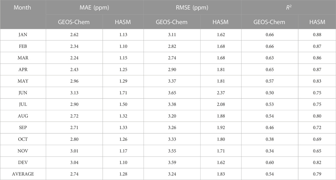
TABLE 1. Monthly error statistics in 2020.

Table 1 lists the monthly error statistics from January to December 2020. The MAEs of the GEOS-Chem simulation data are all greater than 2 ppm. After data fusion using HASM, the MAE at the verification point location is basically below 1.5 ppm. It is slightly higher, at 1.71 ppm, in June but decreases by approximately half from 3.13 ppm in the GEOS-Chem simulation. The RMSEs exhibit the same characteristics, and the RMSEs of the HASM fusion data are all lower than those of the GEOS-Chem simulation data. The monthly R² shows that the fused data have a higher fitting degree to the GOSAT observations. Overall, the annual average MAE and RMSE decreased from 2.74 ppm to 3.24 ppm for the GEOS-Chem simulation data to 1.28 ppm and 1.83 ppm for the HASM fusion data, respectively, and the annual average R² increased from 0.54 before fusion to 0.79 after fusion, indicating that the HASM fusion data have better performance.

The Orbiting Carbon Observatory-2 (OCO-2) and Orbiting Carbon Observatory-3 (OCO-3) from the National Aeronautics and Space Administration (NASA) provide global atmospheric XCO₂ observations with temporal and spatial resolutions of 16 days and 2.25 km × 1.29 km, respectively. The former was launched on 2 July 2014, and the latter was launched on 4 May 2019, and was mounted on the Japanese Experiment Module-Exposed Facility on board the International Space Station (ISS). Here, OCO-2 Level 2 bias-corrected XCO₂ (V11r) and OCO-3 Level 2 bias-corrected XCO₂ (V10.4r), with the quality flag as “0” are used as validation data to compare the XCO₂ data before and after fusion. The fused data are obtained by using all of GOSAT observation data and GEOS-Chem simulations in 2020 through HASM. As shown in Figure 1, HASM fused data presents a lower MAE and RMSE. However, R² also decreases.

FIGURE 1

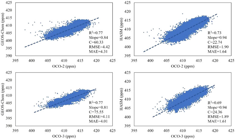
FIGURE 1. Comparison between XCO₂ concentrations from GEOS-Chem/HASM and observations from OCO-2/OCO-3. The coefficient of determination (R²), slope (S), constant (C), root mean square error (RMSE) and mean absolute error (MAE) of the linear regression are indicated in the lower right of the panel.

In the next section, we input all GOSAT data into the HASM data fusion method to obtain monthly global atmospheric XCO₂ concentration data from 2013 to 2021, and conduct spatiotemporal analysis.

3.2 Temporal and spatial variation in global XCO₂ concentration

We calculated the multiyear average global atmospheric XCO₂ concentration from 2013 to 2021 as shown in Figure 2:

FIGURE 2

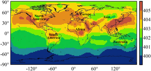
FIGURE 2. Spatial distribution of multiyear global average XCO₂ concentration from 2013 to 2021 (ppm).

Figure 2 shows the global distribution of the multiyear average XCO₂ concentration from 2013 to 2021. The XCO₂ concentration in the Northern Hemisphere is significantly higher than that in the Southern Hemisphere, which is indicative of the influence of human activities. There are also low-value areas of XCO₂ concentrations year-round in some areas of the Northern Hemisphere, such as central North America and the central Eurasian continent. The Southern Hemisphere, with the exception of the Amazon in South America and a small area in central Australia, maintains relatively low concentrations of XCO₂.

We obtained the XCO₂ concentration of HASM at the location of the TCCON site (Park Falls, United States, [90.273°W, 45.945°N]) through bilinear interpolation, and compared it with the observation at this site in Figure 3. Since there are no GOSAT observations for January 2015, the black line is discontinuous that month. Figure 3 shows that the global average concentration of XCO₂ has a clear upwards trend of oscillation with significant seasonality, from approximately 395 ppm in January 2013 to 415 ppm in December 2021. Monthly XCO₂ observations from the TCCON site also show the same change characteristics. For the period from 2019 to 2021, no significant changes can be observed in the global XCO₂ concentration, which is basically consistent with the results of Hwang’s research (Hwang et al., 2021).

FIGURE 3

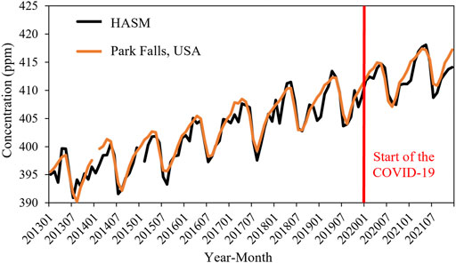
FIGURE 3. Monthly concentration of XCO₂ from the TCCON observations and HASM data fusion for the location of the TCCON site (Park Falls, United States). The red line represents the start of the COVID-19.

3.3 Year-to-year growth in XCO₂ concentration

To examine the growth of atmospheric XCO₂ concentrations before and after the COVID-19 pandemic in more detail, this study compares the year-to-year growth in 2019, 2020, and 2021, using the average year-to-year growth from 2014 to 2018 as the reference growth.

First we calculate the year-to-year growth in each year from 2014 to 2021 using the annual average XCO₂ concentration:

$\begin{array}{l}G{R}_y=D_y-D_{y-1}\end{array}(10)$

where $y$ represents the year (from 2014 to 2021), $G{R}_y$ is the year-to-year growth in the yth year, $D_y$ and $D_{y-1}$ are the annual average XCO₂ concentration in the yth year and the (y-1)-th year. The reference growth is obtained by calculating the average of 2014–2018:

$\begin{array}{l}G{R}_{ref}=\frac{{\sum }_{y=2014}^{2018}G{R}_y}{5}\end{array}(11)$

The relative increase of the year-to-year growth in year $y$ is expressed as follows:

$\begin{array}{l}R\_IN{C}_y=\frac{G{R}_y-G{R}_{ref}}{G{R}_{ref}}\end{array}(12)$

Table 2 shows the comparison of the year-to-year growth of atmospheric XCO₂ and the relative increase in 2019, 2020, and 2021. Globally, the year-to-year growth in 2019 was higher than the reference growth, reaching 2.40 ppm, and the relative increase reached 10.91%. The growth in 2020 was 2.05 ppm, which was 5.20% lower than the reference growth. By 2021, the growth in atmospheric XCO₂ concentration returned to a level that was close to the reference growth. The reference growth and year-to-year growth in 2019, 2020, and 2021 on land were faster than the global growth, at 2.26 ppm, 2.52 ppm, 2.25 ppm and 2.38 ppm respectively. However, when the pandemic emerged in 2020, the year-to-year growth of XCO₂ over the mainland was only slightly lower than that in the multiyear reference. This pattern also proves that the reduction in human activities caused by COVID-19 has not significantly reduced the growth of XCO₂ over the continents as a whole. There are differences in growth across the six continents. In 2020, when the pandemic occurred, the growth on six continents decreased to varying degrees compared with that in 2019, but the growth in Asia and North America were still higher than the reference growth, while in Europe, South America, Australia and Africa, the growth was below the reference growth. In 2021, the growth in Asia, North America, South America, and Europe recovered rapidly, while South Australia and Africa maintained relatively low growth.

TABLE 2

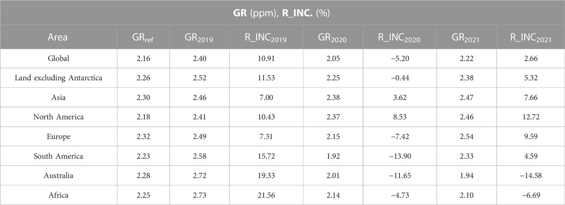
TABLE 2. The year-to-year growth of atmospheric XCO₂ and the relative increase globally and on six continents in 2019, 2020, and 2021.

Figure 4A shows the spatial distribution of the average year-to-year growth of the global XCO₂ concentration from 2013 to 2018. A similar level of growth occurs worldwide, with values of between 2.0 and 2.5 ppm, which also reflects the CO₂ from high-emission areas in the Northern Hemisphere gradually spreading worldwide with atmospheric transport. Figures 4B–D shows the year-to-year growth in 2019, 2020 and 2021. Compared with 2018, the regions on land with faster growth in 2019 were mainly in western North America, Europe, western Siberia in Asia and Southeast Asia. In addition, in the Southern Hemisphere, central South America, Africa and Australia also experienced high growth in XCO₂ concentrations. Compared with 2019, the regions with growth of more than 2.5 ppm in 2020 were significantly reduced, reflecting that in response to the COVID-19 pandemic, the closures and control measures in various countries and regions reduced human activities and CO₂ emissions. At the same time, it can be observed that the areas with higher growth in 2020 were generally opposite to those in 2019, which reflects atmospheric transmission. In 2021, there was a higher degree of growth in North America, and regions with growth of more than 2.5 ppm became larger in Europe, Asia, and South America. In contrast, Africa and Australia did not change greatly and still maintained low XCO₂ growth.

FIGURE 4

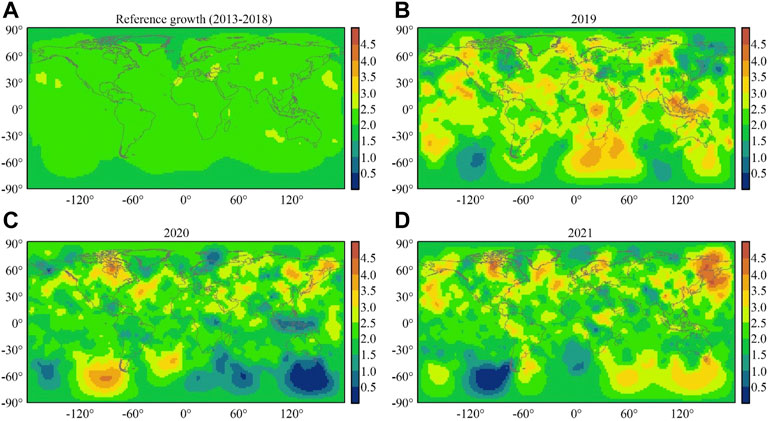
FIGURE 4. Spatial distribution of reference growth and year-to-year growth in 2019, 2020 and 2021 (ppm).

3.4 Growth compared with the same month of the previous year in XCO₂ concentration

Growth compared with the same month of the previous year in XCO₂ concentration are calculated to analyse the growth change in different months of 2019, 2020 and 2021, and the average growth compared with the same month of the previous year from 2013 to 2018 is used as the reference growth. Seasonal and Trend decomposition using Loess (STL) is performed on monthly XCO₂ concentrations to remove seasonal variation in advance.

Growth compared with the same month of the previous year in XCO₂ concentration is calculated as follows:

$\begin{array}{l}G{R}_{m,y}=D_{m,y}-D_{m,y-1}\end{array}(13)$

where $m$ represents the month (from January to December). $y$ represents the year (from 2014 to 2021). $G{R}_{m,y}$ is the growth of the mth month and yth year, $D_{m,y}$ is the deseasonalized atmospheric XCO₂ data of the mth month and yth year, and $D_{m,y-1}$ is the deseasonalized atmospheric XCO₂ data of the mth month and (y-1)-th year.

The reference growth in each month $G{R}_{m,ref}$ and the absolute increase in growth $A\_IN{C}_{m,y}$ are expressed as follows:

$\begin{array}{l}G{R}_{m,ref}=\frac{{\sum }_{y=2014}^{2018}G{R}_{m,y}}{5}\end{array}(14)$

$\begin{array}{l}A\_IN{C}_{m,y}=G{R}_{m,y}-G{R}_{m,ref}\end{array}(15)$

In Figure 5, the dashed, solid, and dotted lines show the absolute increase in growth compared with the same month of the previous year in 2019, 2020 and 2021 at the global level, respectively, using average growth from 2013 to 2018 as the reference growth. In 2019, except for in April, October, and November, the absolute increases in growth were higher than the reference growth, indicating that atmospheric XCO₂ increases rapidly in most months of that year. In 2020, there was a continuous negative value from February to September, indicating that the growth in atmospheric XCO₂ slowed because of COVID-19 prevention measures such as factory shutdowns and city lockdowns. In 2021, the absolute increase of the growth in atmospheric XCO₂ rebounded as a whole, with 7 months having higher growth than the reference growth, reflecting the rapid growth of atmospheric XCO₂ caused by resumed production in various countries.

FIGURE 5

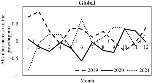
FIGURE 5. The absolute increase in growth compared with the same month of the previous year in 2019, 2020 and 2021 at the global level using average growth from 2013 to 2018 as the reference growth.

Figure 6 shows the absolute increase in growth in 2019, 2020 and 2021 on six continents. Here, the calculations only consider the land area showed in Figure 2. Since most of the world’s economic powerhouses are concentrated in Asia, North America and Europe, the growth in atmospheric XCO₂ on these three continents in the first half of 2020 was lower than that in 2019 to varying degrees, indicating that the COVID-19 pandemic had a significant impact on regional economies in the first half of 2020. Later, with resumed production, carbon emissions gradually returned to normal levels. In Australia and Africa, the growth in 2020 and 2021 were much lower than these in 2019. However, the growth in South America did not show a clear pattern.

FIGURE 6

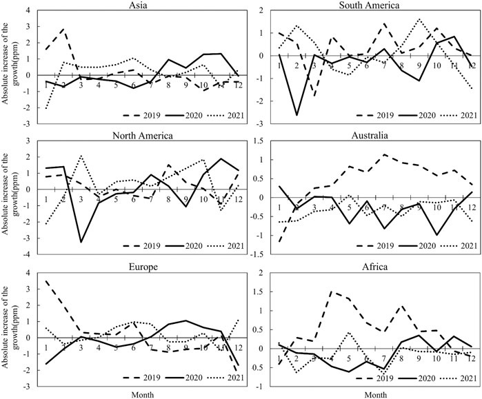
FIGURE 6. The absolute increase in growth compared with the same month of the previous year in 2019, 2020 and 2021 on six continents, using average growth from 2013 to 2018 as the reference growth.

4 Conclusion

This study used HASM to fuse the CO₂ simulation from the atmospheric chemical transport model with XCO₂ observations from GOSAT to obtain global atmospheric XCO₂ concentration fusion data. The accuracy of the fused data were verified, and the characteristics of atmospheric XCO₂ changes under the influence of the COVID-19 pandemic were analysed. The main conclusions of this paper are as follows:

(1) The accuracy of the fused XCO₂ data is greatly improved compared with that of the GEOS-Chem simulation. Cross-validation shows that the average MAE and RMSE of the fused XCO₂ data decreased from from 2.74 ppm to 3.24 ppm before fusion to 1.28 ppm and 1.83 ppm, respectively. R² increased from 0.54 to 0.79. The test results using the observations of OCO-2/OCO-3 as verification points also confirm that the fused data have a lower MAE and RMSE.

(2) Global XCO₂ concentration analysis shows that despite the influence of the COVID-19 pandemic, the global XCO₂ concentration is still rising as a whole, and no significant trend changes can be observed in terms of temporal evolution.

(3) From the perspective of year-to-year growth and growth compared with the same month of the previous year, the COVID-19 pandemic is found to have reduced the growth of atmospheric XCO₂ concentrations on a global scale as a whole in 2020, but the growth gradually recovered and accelerated in 2021. However, growth differed considerably on different continents. In Asia, North America, and Europe, the growth during the COVID-19 outbreak was lower, but then recovered or even exceeded the growth before the outbreak. The growth of XCO₂ in Australia and Africa has remained at a low level after the outbreak, and South America does not show this characteristic pattern.

As it is affected by the spatial resolution of GEOS-Chem, the spatial resolution of the XCO₂ dataset after its fusion with HASM is relatively coarse, and there may be uncertainties in the regional analysis (compared with TCCON observations, HASM misses some small changes in Figure 3). On the other hand, this study mainly focuses on the change in XCO₂ concentrations over land areas, and does not involve the XCO₂ signal over the ocean. There is a time delay in the response of the changes in the high XCO₂ concentrations over the ocean to human activities, so further research is needed on the time window on ocean areas. Even on land, XCO₂ in upwind areas can be transported to downwind areas, causing false anthropogenic signals. For example, the low XCO₂ in Siberia in winter is transported southwards with cold air, reducing the XCO₂ concentrations in eastern China. This may affect the conclusion. In follow-up research, we will consider using the regional atmospheric chemical transport model to improve the spatiotemporal resolution, which will be conducive to a more detailed discussion of the temporal and spatial changes in regional atmospheric XCO₂ under the influence of the COVID-19 pandemic.

Data availability statement

The raw data supporting the conclusion of this article will be made available by the authors, without undue reservation.

Author contributions

YL initial manuscript writing, data analysis, writing the original draft. BW data analysis, supervising, review. TY methodology.

Funding

This work was supported by the Shandong Provincial Natural Science Foundation (ZR2020QD015), a grant from State Key Laboratory of Resources and Environmental Information System, and Major Special Project-the China High-Resolution Earth Observation System (30-Y30F06-9003-20/22).

Acknowledgments

We are grateful for the XCO₂ observations from the NIES GOSAT Projects and OCO-2/OCO-3 Science Team, GEOS-Chem code and drive field from Harvard University, and CO₂ observations from Mauna Loa (HI) Station, which were provided by the research teams on the WDCGG website. We also thank Zhao Mingwei of Chuzhou University for helping with the data processing.

Conflict of interest

The authors declare that the research was conducted in the absence of any commercial or financial relationships that could be construed as a potential conflict of interest.

Publisher’s note

All claims expressed in this article are solely those of the authors and do not necessarily represent those of their affiliated organizations, or those of the publisher, the editors and the reviewers. Any product that may be evaluated in this article, or claim that may be made by its manufacturer, is not guaranteed or endorsed by the publisher.

References

Beck, V., Gerbig, C., Koch, T., Bela, M. M., Longo, K. M., Freitas, S. R., et al. (2013). WRF-chem simulations in the Amazon region during wet and dry season transitions: Evaluation of methane models and wetland inundation maps. Atmos. Chem. Phys. 13 (16), 7961–7982. doi:10.5194/acp-13-7961-2013

CrossRef Full Text | Google Scholar

Buchwitz, M., Reuter, M., Noël, S., Bramstedt, K., Schneising, O., Hilker, M., et al. (2021). Can a regional-scale reduction of atmospheric CO₂ during the COVID-19 pandemic be detected from space? A case study for East China using satellite XCO₂ retrievals. Atmos. Meas. Tech. 14 (3), 2141–2166. doi:10.5194/amt-14-2141-2021

CrossRef Full Text | Google Scholar

Chen, X., Chen, W., Bai, Y., and Wen, X. (2022). Changes in turbidity and human activities along Haihe River Basin during lockdown of COVID-19 using satellite data. Environ. Sci. Pollut. 29 (3), 3702–3717. doi:10.1007/s11356-021-15928-6

PubMed Abstract | CrossRef Full Text | Google Scholar

Connor, B. J., Boesch, H., Toon, G., Sen, B., Miller, C., and Crisp, D. (2008). Orbiting carbon observatory: Inversemethod and prospective error analysis. J. Geophys. Res-Atmos. 113, 1–14. doi:10.1029/2006JD008336

CrossRef Full Text | Google Scholar

Djaferis, T. E., and Schick, I. C. (2000). System theory: Modeling, analysis, and control. Boston: Kluwer.

Google Scholar

Eastham, S. D., Long, M. S., Keller, C. A., Lundgren, E., Yantosca, R. M., Zhuang, J., et al. (2018). GEOS-chem high performance (GCHP v11-02c): A next-generation implementation of the GEOS-chem chemical transport model for massively parallel applications. Geosci. Mod. Dev. 11, 2941–2953. doi:10.5194/gmd-11-2941-2018

CrossRef Full Text | Google Scholar

Fu, Y., Liao, H., Tian, X. J., Gao, H., Jia, B. H., and Han, R. (2021). Impact of prior terrestrial carbon fluxes on simulations of atmospheric CO₂ concentrations. J. Geophys. Res-Atmos. 126 (18). doi:10.1029/2021JD034794

CrossRef Full Text | Google Scholar

Golkar, F., and Mousavi, S. M. (2022). Variation of XCO₂ anomaly patterns in the Middle East from OCO-2 satellite data. Int. J. Digit. Earth. 15 (1), 1218–1234. doi:10.1080/17538947.2022.2096936

CrossRef Full Text | Google Scholar

Hwang, Y. S., Roh, J. W., Suh, D., Otto, M., Schlueter, A., Choudhury, T., et al. (2021). No evidence for global decrease in CO₂ concentration during the first wave of COVID-19 pandemic. Environ. Monit. Assess. 193 (11), 751. doi:10.1007/s10661-021-09541-w

PubMed Abstract | CrossRef Full Text | Google Scholar

Kadygrov, N., Maksyutov, S., Eguchi, N., Aoki, T., Nakazawa, T., Yokota, T., et al. (2009). Role of simulated GOSAT total column CO₂ observations in surface CO₂ flux uncertainty reduction. J. Geophys. Res-Atmos. 114, D21208–D21212. doi:10.1029/2008JD011597

CrossRef Full Text | Google Scholar

Kulawik, S., Wunch, D., O’Dell, C., Frankenberg, C., Reuter, M., Oda, T., et al. (2016). Consistent evaluation of ACOS-GOSAT, BESD-SCIAMACHY, CarbonTracker, and MACC through comparisons to TCCON. Atmos. Meas. Tech. 9, 683–709. doi:10.5194/amt-9-683-2016

CrossRef Full Text | Google Scholar

Kumari, P., and Toshniwal, D. (2020). Impact of lockdown measures during COVID-19 on air quality–A case study of India. Int. J. Environ. Heal. R. 32 (3), 503–510. doi:10.1080/09603123.2020.1778646

PubMed Abstract | CrossRef Full Text | Google Scholar

Kuze, A., Suto, H., Nakajima, M., and Hamazaki, T. (2009). Thermal and near infrared sensor for carbon observation Fourier-transform spectrometer on the greenhouse gases observing satellite for greenhouse gases monitoring. Appl. Opt. 48, 6716–6733. doi:10.1364/AO.48.006716

PubMed Abstract | CrossRef Full Text | Google Scholar

Lau, H., Khosrawipour, V., Kocbach, P., Mikolajczyk, A., Schubert, J., Bania, J., et al. (2020). The positive impact of lockdown in Wuhan on containing the COVID-19 outbreak in China. J. Travel Med. 27 (3), taaa037–7. doi:10.1093/jtm/taaa037

PubMed Abstract | CrossRef Full Text | Google Scholar

Le Quéré, C., Jackson, R. B., Jones, M. W., Smith, A. J. P., Abernethy, S., Andrew, R. M., et al. (2020). Temporary reduction in daily global CO₂ emissions during the COVID-19 forced confinement. Nat. Clim. Chang. 10, 647–653. doi:10.1038/s41558-020-0797-x

CrossRef Full Text | Google Scholar

Lian, J., Lauvaux, T., Utard, H., Bréon, F., Broquet, G., Ramonet, M., et al. (2022). Assessing the effectiveness of an urban CO₂ monitoring Network over the paris region through the COVID-19 lockdown natural experiment. Environ. Sci. Tech. 56 (4), 2153–2162. doi:10.1021/acs.est.1c04973

PubMed Abstract | CrossRef Full Text | Google Scholar

Liu, Y., Yue, T. X., Zhang, L. L., Zhao, N., Zhao, M. M., and Liu, Y. (2018). Simulation and analysis of XCO₂ in North China based on high accuracy surface modeling. Environ. Sci. Pollut. Res. 25 (27), 27378–27392. doi:10.1007/s11356-018-2683-x

PubMed Abstract | CrossRef Full Text | Google Scholar

Liu, Z., Deng, Z., Zhu, B. Q., Ciais, P., Davis, S. J., Tan, J. G., et al. (2022). Global patterns of daily CO₂ emissions reductions in the first year of COVID-19. Nat. Geosci. 15, 615–620. doi:10.1038/s41561-022-00965-8

CrossRef Full Text | Google Scholar

Masson-Delmotte, V., Zhai, P., Pirani, A., Connors, S. L., Pean, C., Chen, Y., et al. (2021). Climate change 2021: The physical science basis. Contribution of working group I to the sixth assessment report of the intergovernmental panel on climate change. Available at: https://www.ipcc.ch/report/ar6/wg1/downloads/report/IPCC_AR6_WGI_FrontMatter.pdf.

Google Scholar

Murray, L. T., Leibensperger, E. M., Orbe, C., Mickley, L. J., and Sulprizio, M. (2021). GCAP 2.0: A global 3-D chemical-transport model framework for past, present, and future climate scenarios. Geosci. Model. Dev. 14, 5789–5823. doi:10.5194/gmd-14-5789-2021

CrossRef Full Text | Google Scholar

Park, R. J., Jacob, D. J., Field, B. D., Yantosca, R. M., and Chin, M. (2004). Natural and transboundary pollution influences on sulfate-nitrate-ammonium aerosols in the United States: Implications for policy. J. Geophys. Res. 109, D15204. doi:10.1029/2003JD004473

CrossRef Full Text | Google Scholar

Park, S., Shin, J., Kim, S., Oh, E., and Kim, Y. (2019). Global climate simulated by the Seoul National University atmosphere model version 0 with a unified convection scheme (SAM0-UNICON). J. Clim. 32 (10), 2917–2949. doi:10.1175/JCLI-D-18-0796.1

CrossRef Full Text | Google Scholar

Peng, Z., Zhang, M., Kou, X., Tian, X., and Ma, X. (2015). A regional carbon data assimilation system and its preliminary evaluation in East Asia. Atmos. Chem. Phys. 15, 1087–1104. doi:10.5194/acp-15-1087-2015

CrossRef Full Text | Google Scholar

Peters, W., Jacobson, A. R., Sweeney, C., Andrews, A. E., Conway, T. J., Masarie, K., et al. (2007). An atmospheric perspective on North American carbon dioxide exchange: CarbonTracker. Proc. Natl. Acad. Sci. USA/PNAS 104, 18925–18930. doi:10.1073/pnas.0708986104

PubMed Abstract | CrossRef Full Text | Google Scholar

Shi, W. J., Liu, J. Y., Du, Z. P., Stein, A., and Yue, T. X. (2011). Surface modelling of soil properties based on land use information. Geoderma 162, 347–357. doi:10.1016/j.geoderma.2011.03.007

CrossRef Full Text | Google Scholar

Shi, W. J., Yue, T. X., Du, Z. P., Wang, Z., and Li, X. W. (2016). Surface modeling of soil antibiotics. Sci. Total. Environ. 543, 609–619. doi:10.1016/j.scitotenv.2015.11.077

PubMed Abstract | CrossRef Full Text | Google Scholar

Shiomi, K., Kikuchi, N., Suto, H., Kataoka, F., and Kuze, A. (2022). “Gosat partial column observation for better quantifying urban CO₂ flux,” in IGARSS 2022-2022 IEEE International Geoscience and Remote Sensing Symposium (Kuala Lumpur, Malaysia: IEEE), 4350–4352. doi:10.1109/IGARSS46834.2022.9884603

CrossRef Full Text | Google Scholar

Somasundaram, D. (2005). Differential geometry. Harrow: Alpha Science International.

Google Scholar

Sussmann, R., and Rettinger, M. (2020). Can we measure a COVID-19-related slowdown in atmospheric CO₂ growth? Sensitivity of total carbon column observations. Remote Sens. 12 (15), 2387. doi:10.3390/rs12152387

CrossRef Full Text | Google Scholar

Wang, L., Wang, J., Fatholahi, S. N., Chapman, M. A., Chen, Y., and Li, J. (2022). “Assessing the impact of covid-19 on human activities in the greater toronto area by nighttime light images and active covid-19 cases,” in IGARSS 2022-2022 IEEE International Geoscience and Remote Sensing Symposium (Kuala Lumpur, Malaysia: IEEE), 7847–7850. doi:10.1109/IGARSS46834.2022.9884325

CrossRef Full Text | Google Scholar

Wang, Y. F., Yue, T. X., Lei, Y. C., Du, Z. P., and Zhao, M. W. (2016). Uncertainty of forest biomass carbon patterns simulation on provincial scale: A case study in jiangxi province, China. J. Geogr. Sci. 26, 568–584. doi:10.1007/s11442-016-1286-z

CrossRef Full Text | Google Scholar

Weir, B., Crisp, D., O’Dell, C. W., Basu, S., Chatterjee, A., Kolassa, J., et al. (2021). Regional impacts of COVID-19 on carbon dioxide detected worldwide from space. Sci. Adv. 7 (45), eabf9415. doi:10.1126/sciadv.abf9415

PubMed Abstract | CrossRef Full Text | Google Scholar

Yue, T. X. (2011). Surface modeling: High accuracy and high speed methods. Boca Raton, FL, USA: CRC Press. doi:10.1201/b10392

CrossRef Full Text | Google Scholar

Yue, T. X., Liu, Y., Zhao, M. W., Du, Z. P., and Zhao, N. (2016b). A fundamental theorem of Earth’s surface modelling. Environ. Earth. Sci. 75, 751. doi:10.1007/s12665-016-5310-5

CrossRef Full Text | Google Scholar

Yue, T. X., Zhang, L. L., Zhao, M. W., Wang, Y. F., and Wilson, J. P. (2016a). Space-and ground-based CO₂ measurements: A review. Sci. China Earth Sci. 59, 2089–2097. doi:10.1007/s11430-015-0239-7

CrossRef Full Text | Google Scholar

Yue, T. X., Zhao, N., Liu, Y., Wang, Y. F., Zhang, B., Du, Z. P., et al. (2020). A fundamental theorem for eco-environmental surface modelling and its applications. Sci. China Earth Sci. 63 (8), 1092–1112. doi:10.1007/s11430-019-9594-3

CrossRef Full Text | Google Scholar

Yue, T. X., Zhao, N., Ramsey, D., Wang, C. L., Fan, Z. M., Chen, C. F., et al. (2013). Climate change trend in China, with improved accuracy. Clim. Chang. 120, 137–151. doi:10.1007/s10584-013-0785-5

CrossRef Full Text | Google Scholar

Zhang, H., Ma, X., Han, G., Xu, H., Shi, T., Zhong, W., et al. (2021). Study on collaborative emission reduction in green-house and pollutant gas due to COVID-19 lockdown in China. Remote Sens. 13 (17), 3492. doi:10.3390/rs13173492

CrossRef Full Text | Google Scholar

Zhao, N., Yue, T., Li, H., Zhang, L. L., Yin, X. Z., and Liu, Y. (2018). Spatio-temporal changes in precipitation over Beijing-Tianjin-Hebei region, China. Atmos. Res. 202, 156–168. doi:10.1016/j.atmosres.2017.11.029

CrossRef Full Text | Google Scholar