A study of the nonlinear dynamic interrelationship between CO2 emissions and logistics sector output growth

Using provincial panel data spanning from 1995 to 2020, this paper examines the nonlinear interrelationship between logistics carbon dioxide emissions and output growth. For this purpose, we conduct a nonlinear co-integration test in heterogeneous panels; our results suggests a long-run relationship between these two variables. In contrast, adjustment to the equilibrium is inherently nonlinear. Furthermore, we estimate a panel smooth transition vector error correction model. Our major contributions, as we know, are the first study confirming the existence of a dynamic mechanism between logistics carbon dioxide emissions and regional output growth and the Environmental Kuznets Curve in China. Last, the interaction between logistics carbon dioxide emissions and regional output growth varies over the output growth in Chinese provinces and autonomous regions. Our results highlight the importance of considering possible nonlinearities in analyzing output-carbon dioxide emissions causality nexus and designing energy policies.

Introduction

In recent years, global warming and environmental pollution have renewed interest in the low-carbon economy, which has primarily been discussed by the Chinese government and academic communities. China is responsible for 15% of global greenhouse gas emissions, of which CO₂ emissions make up 80%.

In the past decade, the average annual growth rate of CO₂ emissions has been 17.8% in China, which is at the forefront of the world (Zhao and Hu, 2013). The Chinese government pledged at the Paris Conference on Climate Changes in November 2015 that carbon dioxide emissions would peak around 2030. In April 2016, China formally ratified the Paris Agreement, and in September 2020, the 75th United Nations General Assembly vowed to take stronger action and work toward becoming carbon neutral before 2060.

However, China is still under intense pressure to reduce emissions in order to meet this target.

Logistics is a high-energy-consuming industry that also generates a significant amount of CO₂ emissions. In China, the logistics sector has emerged as one of the biggest consumers of energy resources, according to Xu and Yu’s calculation of the CO₂ emissions of the industry in 2020.

According to the International Energy Agency’s 2009 report “Transport, Energy, and Carbon Emissions: Towards Sustainability,” the transportation sector accounts for approximately 25% of global CO₂ emissions. In light of this, all counties are working toward creating a cleaner logistics sector. To address these worries. Alinaghian and Goli (2017) proposed an uncertain integrated model for locating temporary depots in affected areas, allocating affected areas to these centres, and routing required goods through such centres.

The proposed model pursued to reduce the time required to reach the last relief centre. Goli et al. (2021) specifically address the prediction of dairy product demand to improve logistics systems for dairy product transportation, allowing for a brief consumption period, as a result of their insights into green logistics. Furthermore, Tirkolaee et al. (2022) developed a novel mathematical model based on Pareto-based algorithms to design a sustainable mask Closed-Loop Supply Chain Network during the COVID-19 outbreak for the first time. Their efforts contribute to the reduction of environmental degradation through green transportation.

Our research here is primarily connected to two strands of the literature. The first strand concerns to the existence of the Environmental Kuznets Curve, which has piqued the interest of academics, practitioners, and regulators since Kyoto Protocol was signed.

Understanding the link between CO₂ emissions and economic growth helps economies in developing energy policies and sustainable energy resources. Pao and Tsai (2010) studied the relationship between pollutant emissions, energy consumption and output growth in BRIC countries. This study shows that energy consumption has a positive long-term effect on CO₂ emissions, being statistically significant. In contrast, the relationship between actual output and CO₂ emissions shows an inverted U-shaped relationship with a threshold income effect. Wang et al. (2011) used a data set of 28 provinces in China. They found that there is an inverted U-shaped relationship between CO₂ emissions in energy consumption and output growth by a panel co-integration test. They ascribed higher per capita CO₂ emissions in China to the overuse of energy resources. Using a data set from 12 countries in the Middle East and North Africa, Arouri et al. (2012) showed that energy consumption influences CO₂ emissions positively in the long run. A quadratic relationship exists between actual GDP and CO₂ emissions, confirming the EKC hypothesis. Based on the autoregressive distributed lag model, Baek and Kim (2013) confirmed that the EKC relationship held in South Korea over the past 40 years. Recently, Khan and Eggoh (2021) re-assessed the relationship between economic growth and pollution emissions using a large panel of 146 economies from 1990 to 2016. Their empirical findings support the existence of the Environmental Kuznets Curve hypothesis for the global sample as well as for income-specific sub-samples. Rahman et al. (2020) investigates the impact of CO₂ emissions, population density, and trade openness on the economic growth of five South Asian countries from 1990 to 2017. The obtained results reveal that CO₂ emissions and population density positively, and trade openness negatively affect the economic growth in South Asia. Further, Anwar et al. (2022) investigated the major determinants of CO₂ emissions in Far East countries in the period of 1980–2017, finding that urbanization, economic growth and trade openness significantly determine CO₂ emission in the selected countries.

Although in recent years, numerous studies have thoroughly investigated the nexus between economic growth and CO₂ emissions, and concluded a positive relationship between CO₂ emissions and economic growth in various degrees, many studies conclude quite different from the conventional view. Lu (2000) specified a state-space model between per capita carbon emissions and per capita GDP and found that the relationship between the two is not simply inverted U-shaped but tells a more complicated story. Choi et al. (2010) explored the EKC relationship between China, a newly industrialized country, South Korea, and Japan, a developed economy, using data from 1971 to 2006. Their findings suggest that the EKC relationship exhibits different temporal patterns across different countries, which vary according to the countries level of economic development.

The results show that China has an N-shaped curve, Japan has a U-shaped curve, and Korea has an inverted U-shaped curve. Wang (2012) conducted the most comprehensive study (98 countries involved), examining the non-linear relationship between CO₂ emissions from oil and GDP while accounting for population growth. This study found that a threshold effect exists in the relationship between emissions and growth and it was concluded that the impact of CO₂ emissions varies from low-income to wealthy countries. Similarly, Li and Ya (2012) investigated the long-term equilibrium relationship between the carbon emissions from China’s manufacturing, construction, and transportation industries and output growth from the standpoint of harmoniously industrial development. CO₂ emissions stimulate economic growth in the short term, but their influence gradually fades and finally becomes stationary in the long term. The contribution of CO₂ emissions from the transportation and construction industries to economic growth decreases initially before increasing as a result of the industrial adjustment. Muhammad (2019) examined the link between economic growth, energy consumption and CO₂ emissions for the panel of 68 countries between 2001–2017, that included developed, emerging and Middle East and North Africa (MENA) countries. Economic growth in developed and emerging countries increased energy consumption, while declining in MENA countries; due to an increase in energy consumption CO₂ emissions increased in all countries.

Adebayo et al. (2021) re-examine the relationship between urbanization, CO₂ emissions, gross capital formation, energy use, and economic growth in South Korea using data from 1965 to 2019, finding that CO₂ emissions trigger economic growth and that the energy-induced growth hypothesis is validated, but the EKC relationship collapses. Sun et al. (2021) examined the dynamic relationship between carbon emissions, trade, energy consumption, urbanization, and output growth from 1992 to 2015. The Environmental Kuznets Curve (EKC) assumption is confirmed only in three panels, and output growth has a significant positive effect on environmental pollution in all panels.

The second strand is associated with the nexus between CO₂ emissions and output growth in the logistics industry. Abbes and Bulteau (2018) investigates the dynamic effects of GDP growth, motorization rate, transport pollution coefficient, and energy intensity on CO₂ emissions from the transport sector in Tunisia. In the long run, the statistically insignificant effects of per capita GDP on transport carbon emissions in the long run suggest that these emissions can be controlled without disrupting economic growth.This can be accomplished by developing short-sea shipping between major cities in order to reduce traffic congestion and carbon emissions.

Liu et al. (2019) examine the impact of income and region on environmental logistics performance index scores and discuss the potential for reduction in oil consumption intensity and carbon intensity in those countries. The main finding is that the environmental logistics performance index generally perform well in the environmental logistics performance index.

The environmental logistics performance index, like the logistics performance index, is closely related to income and region. Similar to the characteristics of the logistics performance index, the environmental logistics performance index is also closely related to income and region. Liu et al. (2021) employ a Global Malmquist-Luenberger Index approach to evaluate the green productivity growth of road transportation in China at the provincial level based on the Data Envelopment Analysis and Directional Distance Function, finding that, at the regional level, the road transportation industries in Western and Central China achieved green productivity growth because of the catch-up effect and the economies of scale, respectively. Wang (2021) confirms that, with the growth of GDP per capita, the degree of coupling and coordination between the logistics and financial industries has promoted the increase of carbon emissions in various regions. Still, the promotion effect is an inverted U-shaped trend that first increases and then decreases. Recently, Awan et al. (2022) investigate the nexus between transport sector-based carbon dioxide emissions, economic growth, innovation, and urbanization. Furthermore, the study analyzes the Environmental Kuznets Curve (EKC) hypothesis for the transport sector in balanced panel data of 33 high-income countries from 1996 to 2014 using a robust and novel quantile methodology. Findings reveal the validity of an N-shape EKC curve for the transport sector. The study recommends shifting to public transportation systems to help curb environmental degradation through green transportation. Aydin et al. (2022) investigate the impact of energy intensity on the relationship between logistic growth and environmental pollution in 45 countries that support the One Belt One Road project proposed to revitalize the historical Silk Road between 2007 and 2018. According to the findings of the study, the relationship between logistics growth and environmental pollution is not linear, and energy intensity level plays an important role in this relationship (Tirkolaee et al., 2022). Hassan et al. (2022) examine the dynamic linkage among nuclear energy, public service transportation, real income, and innovative technology with CO₂ emissions in China. Results show that innovative technology mitigates environmental pollution. As a result, different perspectives from previous studies lead to different theoretical insights into the relationship between output growth and CO₂ emissions, and no definitive policy framework exists to address the escalating problem of greenhouse gas emissions. Furthermore, in the logistics sector, the existing literature focuses primarily on different aspects of logistics such as transportation (Fleisher and Chen, 1997; Lu et al., 2019), and telecommunication (Jing and Ab-Rahim, 2020).

However, the literature lacks a deeper examination of the logistics sector’s output using a large panel dataset. Most of relevant studies focus on the relationship between energy consumption and output growth at a national level. Yuan et al. (2008) discovered a co-integration relationship between energy consumption and output growth between 1978 and 2004. Other studies concentrate on a large number of countries at the same time. Li et al. (2021) investigate the economic and environmental impacts of green logistics performance for One Belt and Road Initiative (OBRI) countries from 2007 to 2019. According to the findings, green logistics performance improves OBRI economic growth while enhancing environmental pollution in these countries. Their studies, however, assume that model parameters do not change over time and, as a result, ignore China’s heterogeneity across regions, which is one of the main causes of estimation bias. To overcome the limitations of their studies, we use the panel smooth transition regression model (PSTR) proposed by Gonzalez et al. (2005). This model is lent to analyze the relationship between CO₂ emissions and output growth of the logistics sector in different regions to investigate the heterogeneity and time-varying parameters of the PSTR model across regions. It is of great significance to clarify the debate on whether an EKC relationship exists between CO₂ emissions of the logistics sector and output growth based on our econometric framework.

Econometric framework

Nonlinear panel co-integration test

Consider the following panel regression model:

$y_{i,t}={\alpha }_i+{\beta }_i{x}_{i,t}+u_{i,t}(1)$

where $i=1,\cdots ,N$, $t=1,\cdots ,T$, $y_{i,t}$ and $x_{i,t}$ represent the observed $I\left(1\right)$ variables, $\beta =\left({\beta }_1,{\beta }_2,\cdots ,{\beta }_m\right)$ are the parameters to be estimated, $u_{i,t}$ is the error term, $y_{i,t}$ is a scalar, $x_{i,t}=\left(x_{1,t},x_{2,t},\cdots ,x_{m,t}\right)$ is a $\left(m\times 1\right)$ vector, and ${\alpha }_i$ symbolizes individual fixed effect. Further, suppose that a $\left(n\times 1\right)$ vector $z_{i,t}^{\prime }=\left(y_{i,t},\cdots ,x_{i,t}\right)$ is generated by a process $z_{i,t}=z_{i,t-1}+{\epsilon }_{i,t}$, where ${\epsilon }_{i,t}$ is a error term with zero mean and a positively definite variance covariance matrix, and $E{\left({\epsilon }_{i,t}\right)}^s<\infty ,$ for $s>4$.

If the error term $u_{i,t}$ is stationary in Eq. 1, the vector $z_{i,t}$ is co-integrated, $u_{i,t}$ is called the equilibrium error. In this paper, we assume that $u_{i,t}$ can be generated using the following non-linear process:

$u_{i,t}={\gamma }_i{u}_{i,t-1}+{\psi }_i{u}_{i,t-1}F\left(u_{i,t-1};{\theta }_i\right)+{\xi }_{i,t}(2)$

Where ${\xi }_{i,t}$ is the error of zero mean, and $F\left(u_{i,t-1};{\theta }_i\right)$ is a smooth transition function of $u_{i,t}$. According to the previous literature (e.g. Kapetanios et al., 2003; Kapetanios et al., 2006; Maki, 2010) dealing with the nonlinear co-integrated relationship, we assume a exponential transition function $F\left(u_{i,t-1};{\theta }_i\right)$ as follows,

$F\left(u_{i,t-1};{\theta }_i\right)=1-\exp \left\{-{\theta }_i{u}_{i,t-1}^2\right\}(3)$

Furthermore, assume that $u_{i,t}$ follows a stochastic process with zero mean, and the parameter ${\theta }_i$ determines the speed at which the function changes its values from an extreme to another. A exponential function has excellent properties that the speed at which its values are adjusted to a long-run equilibrium state depends on the degree of the disequilibrium. Substituting Eq. 3 into Eq. 2 and reparameterizing Eq. 2, we obtain the following model:

$\Delta u_{i,t}={\phi }_i{u}_{i,t-1}+{\psi }_i{u}_{i,t-1}\left[1-\exp \left\{-{\theta }_i{u}_{i,t-1}^2\right\}\right]+{\zeta }_{i,t}(4)$

Imposing a constraint on Eq. 4 that $u_{i,t}$ follows the unit root process in the medium regime, i.e. ${\phi }_i=0$, and further considering the possible sequential correlation of the error terms in Eq. 4, we obtain a regression model as follows:

$\Delta u_{i,t}={\psi }_i{u}_{i,t-1}\left[1-\exp \left\{-{\theta }_i{u}_{i,t-1}^2\right\}\right]+{\displaystyle \sum }_{j=1}^p{\rho }_{ij}{u}_{i,t-j}+{\zeta }_{i,t}(5)$

The test of co-integration is based on the parameter ${\theta }_i$, which is equal to 0 under null hypothesis of the presence of the co-integration relationship, and is positive under alternative hypothesis. However, it is not feasible to test null hypothesis directly, since the parameter ${\psi }_i$ is unidentified under null hypothesis. According to Luukkonen et al. (1988)’s methodology dealing with this problem, the first-order Taylor expansion can be applied to the transition function Eq. 3.

Under null hypothesis, the first-order Taylor approximation yields the following auxiliary regression equation:

$\Delta u_{i,t}={\delta }_i{u}_{i,t-1}^3+{\displaystyle \sum }_{j=1}^{p_i}{\rho }_{ij}\Delta u_{i,t-j}+e_{i,t}(6)$

where $e_{i,t}$ is composed of the disturbance term and Taylor approximation error in Eq. 5. In regression Eq. 6, each term is allowed to have a different lag order $p_i$. Specifically, the null and alternative hypotheses can be expressed, respectively, as:

$H_0:{\delta }_i=0$, for all $i$, implies no co-integration relationship;

$H_1:{\delta }_i<0$, for some $i$, implies that a nonlinear co-integration relationship exists.

In practice, an appropriate lag order should be selected for the auxiliary regression model Eq. 6. Following Uçar and Omay (2009), the average of the co-integration test statistics is first taken over the entire panel data, and then the nonlinear panel co-integration test statistics can be computed. The standardized $t$ statistic (see Kapetanios et al., 2003) is defined as:

$t_{i,NL}=\frac{\Delta u_i^{\prime }{M}_t{u}_{i,-1}^3}{{\widehat{\sigma }}_{i,NL}{\left(u_{i,-1}^{\prime }{M}_t{u}_{i,-1}\right)}^{3/2}}(7)$

where ${\widehat{\sigma }}_{i,NL}^2=\frac{∆u_i^{\prime }{M}_t{u}_i}{T-1}$, $M_t=I_T-{\tau }_T{\left({\tau }_T^{\prime }{\tau }_T\right)}^{-1}{\tau }_T^{\prime }$, $∆u_i={\left(∆u_{i,1},∆u_{i,2},\cdots ,∆u_{i,T}\right)}^{\prime }$, and ${\tau }_T=\left(\mathrm{1,1},\cdots ,1\right)$.

According to Pesaran (2007), we use the t statistic in Eq. 7 to compute the panel unit root test statistic, and ${\overline{t}}_{NL}$ statistic can be symbolized as follows:

$\overline{t}\left(N,T\right)=\frac{1}{N}{\displaystyle \sum }_{i=1}^N{t}_i\left(N,T\right)(8)$

A common obstacle encountered in panel regression is the presence of cross-section interdependence, which invalidate traditional unit root and co-integration tests. This paper follows the methodology proposed by Pesaran (2004), whose test statistic is represented as:

$CD=\sqrt{\frac{2T}{N\left(N-1\right)}}\left({\displaystyle \sum }_{i=1}^{N-1}{\displaystyle \sum }_{j=i+1}^N{\widehat{\rho }}_{ij}\right)(9)$

where ${\widehat{\rho }}_{ij}$ is the correlation coefficient between the error terms of Eq. 1 for individuals $i$ and $j$. Using the Uçar and Omay (2009)’s method, this paper applies Sieve bootstrap to deal with cross-section dependence. Considering that the long-term equilibrium relationship and the short-term dynamic relationship between variables might be potentially nonlinear, we propose a nonlinear panel smooth transition vector error correction model (PSTRVEC) to study the regime dependent relationship between CO₂ emissions from the logistics sector and output growth. We turn to the specification and estimation of the PSTRVEC model in the next subsection.

Nonlinear panel smooth transition vector error correction model

According to Gonzalez et al. (2005), we specify the panel smooth transition vector error correction model (PSTRVEC) as follows:

$\begin{array}{ll}\hfill \Delta gdp& ={\mu }_{1i}+{\beta }_{1}e{c}_{1i,t-1}+{\displaystyle \sum }_{j=1}^{p_i}{\theta }_{1j}\Delta gd{p}_{i,t-j}+{\displaystyle \sum }_{j=1}^{q_i}{\vartheta }_{1j}\Delta C{O}_{2i,t-j}\hfill \\ \hfill & +G\left(S_{i,t};\gamma ,c\right)\{{\stackrel{\sim }{\beta }}_{1}e{c}_{1i,t-1}+{\displaystyle \sum }_{j=1}^{p_i}{\stackrel{\sim }{\theta }}_{1j}\Delta gd{p}_{i,t-j}+{\displaystyle \sum }_{j=1}^{q_i}{\stackrel{\sim }{\vartheta }}_{1j}\Delta C{O}_{2i,t-j}\}\hfill \\ \hfill & +{\xi }_{1it}\Delta C{O}_{2i,t}={\mu }_{2i}+{\beta }_{2}e{c}_{2i,t-1}+{\displaystyle \sum }_{j=1}^{r_i}{\theta }_{2j}\Delta gd{p}_{i,t-j}+{\displaystyle \sum }_{j=1}^{s_i}{\vartheta }_{2j}\Delta C{O}_{2i,t-j}\hfill \\ \hfill & +G\left(S_{i,t};\gamma ,c\right)\{{\stackrel{\sim }{\beta }}_{2}e{c}_{2i,t-1}+{\displaystyle \sum }_{j=1}^{r_i}{\stackrel{\sim }{\theta }}_{2j}\Delta gd{p}_{i,t-j}+{\displaystyle \sum }_{j=1}^{s_i}{\stackrel{\sim }{\vartheta }}_{2j}\Delta C{O}_{2i,t-j}\}+{\xi }_{2it}\hfill \end{array}(10)$

for $i=1,\dots ,N$, and $t=1,\dots ,T$, where $N$ and $T$ denotes the cross-section and time dimensions of the panel, respectively; $gd{p}_{i,t}$ is output in the logistics industry; while $C{O}_{2i,t}$ symbolizes the carbon dioxide emissions of logistics industry. ${\mu }_{1i}$ and ${\mu }_{2i}$ capture fixed individual effects; $e{c}_{1i,t}$ and $e{c}_{2i,t}$ are the error correction terms¹ from regression Eq. 1; ${\xi }_{li,t}$ and ${\xi }_{2i,t}$ are disturbance terms assumed to be martingale difference processes with respect to the history of the variables with mean zero and variance, ${\sigma }_i^2$. We consider that the errors of $N$ equations have a simultaneous correlation (namely, $\mathrm{c}\mathrm{o}\mathrm{v}\left({\xi }_{li,t},{\xi }_{lj,t}\right)\ne 0$, $l=\mathrm{1,2}$ for $i\ne j$).

To model regime-shifts in the short-run and long-run, Gonzalez et al. (2005) and Omay and Kan (2010) consider the employment of the following logistic transition function:

$G\left(S_{i,t};\gamma ,c\right)={\left[1+\exp \left\{-\gamma \stackrel{m}{\underset{j=1}{\mathrm{\Pi }}}\left(S_{i,t}-c_j\right)\right\}\right]}^{-1},\gamma >0,c_m\ge \cdots \ge c_1\ge c_0(11)$

where $c={\left(c_1,\cdots ,c_m\right)}^{\prime }$ is a $m$-dimensional vector of location parameters and the slope parameter, $\gamma$, denotes the smoothness degrees between regimes. $m=$ 1 or 2 usually meet usual modes of regime-shifts. When $m=$ 1, Eq. 11 is the first-order logistic transition function, and the extreme regimes correspond to the maximum and minimum of the transition variable $S_{i,t}$. As $S_{i,t}$ increases, the coefficients of the PSTRVEC model (10) transit smoothly from ${\beta }_j$, ${\theta }_j$ and ${\vartheta }_j$ to ${\beta }_j+{\stackrel{\sim }{\beta }}_j$, ${\theta }_j+{\stackrel{\sim }{\theta }}_j$ and ${\vartheta }_j+{\stackrel{\sim }{\vartheta }}_j$ respectively. When $\gamma \to \infty$, the first-order logistic transition function $G\left(S_{i,t};\gamma ,c\right)$ becomes an indicator function $I\left[A\right]$. When an event $A$ occurs, it is valued at 1; otherwise, it is equal to 0. Hence, the PSTRVEC model is simplified into the two-regime threshold model (Hansen, 1999).

For $m=2$, on the other hand, the logistic transition function takes a value of 1 for both low and high values of $S_{it}$, minimizing at $\left(c_1+c_2\right)/2$. In such a case, if $\gamma \to \infty$, the model reduces to a three-regime panel threshold model. In contrast, if $\gamma \to 0$, the transition function $G\left(S_{i,t};\gamma ,c\right)$ is a constant, therefore, the PSTRVEC model is simplified into a linear panel regression model. The specification and estimation of the PSTRVEC model follow the following steps:

Firstly, specify an appropriate linear panel model which fits the selected data excellently; Secondly, test null hypothesis of a linear panel model. If linearity is rejected, select an appropriate transition variable $S_{i,t}$ and a form of transition function; Finally, estimate the specified PSTRVEC model.

In the second step above, the complexity of testing null of linearity results from unidentified ‘notorious’ parameters under null hypothesis. To overcome this problem, the transition function may be replaced with the appropriate Taylor approximation (Luukkonen et al., 1988). For example, the $k^{th}$ order Taylor approximation of the first-order logistic transition function around $\gamma =0$ results in the following auxiliary regression:

$\Delta z_{i,t}={\lambda }_i+{\pi }_0^{,}e{c}_{i,t-1}+{\displaystyle \sum }_{j=1}^{p_i}{\psi }_{0j}\Delta z_{i,t-j}+{\displaystyle \sum }_{h=1}^k{\stackrel{\sim }{\pi }}_h^{,}{S}_{i,t}^{h}e{c}_{i,t-1}+{\displaystyle \sum }_{h=1}^k{\displaystyle \sum }_{j=1}^{p_i}{\stackrel{\sim }{\psi }}_{hj}{S}_{i,t}^h\Delta z_{i,t-j}+e_{i,t}(12)$

where $z_{i,t}={\left(gd{p}_{i,t},C{O}_{2i,t}\right)}^{\prime }$, and $\lambda ,{\pi }^{\prime },\psi ,\stackrel{\sim }{\pi }$ and $\stackrel{\sim }{\psi }$ is reparameterization of original parameters ${\mu }_i,\beta ,{\theta }_j,{\vartheta }_j,\stackrel{\sim }{\beta },{\stackrel{\sim }{\theta }}_j,{\stackrel{\sim }{\vartheta }}_j,\gamma$ and $c_i$ respectively; $e_{i,t}$ consists of the original disturbance term ${\xi }_{i,t}$ and errors from the Taylor approximation. Thus, testing null hypothesis $H_0:\gamma =0$ in (10) is equivalent to testing null hypothesis $H_0$: ${\omega }_1={\omega }_2={\omega }_3=0$, where ${\omega }_1,{\omega }_2,{\omega }_3$ corresponds to ${\omega }_i\equiv \left({\stackrel{\sim }{\pi }}_i,{\stackrel{\sim }{\psi }}_i\right)$ in Eq. 12, respectively. LM test is desired to test null hypothesis, which approximately follows a F distribution:

$LM=\frac{\left(SS{R}_0-SS{R}_1\right)/kp}{SS{R}_0/\left(TN-N-k\left(p+1\right)\right)}\sim F\left(kp,TN-N-k\left(p+1\right)\right)(13)$

where $SS{R}_0$ and $SS{R}_1$ is the sum of the squares of residuals under null hypothesis and alternative hypothesis, respectively. In order to select an appropriate transition variable $S_{i,t}$, LM statistics can be calculated using different transition variables, where the transition variable with the lowest p-value accompanying the LM statistic should be selected to estimate Eq. 12.

When the transition variable $S_{i,t}$ is selected appropriately, the next step is to choose $m=1$ or $m=2$. Teräsvirta, 1994 suggests using various inference rules for Eq. 12. Following these rules, we test null hypothesis $H_0^{*}$: ${\omega }_1={\omega }_2={\omega }_3=0$ by estimating the auxiliary regression Eq. 12 with $k=3$. If it is rejected, we test null hypothesis $H_{03}^{*}:{\omega }_3=0$. If $H_{03}^{*}$ is rejected, other null hypothesis are tested further, $H_{02}^{*}:{\omega }_2=0|{\omega }_3=0$, and $H_{01}^{*}:{\omega }_1=0|{\omega }_2={\omega }_3=0$, respectively. These tests are inferred using F statistic, denoted as $F,F_3,F_2$ and $F_1$, respectively. Finally, the inference proceeds as follows: If the p-value associated with $F_2$ is minimum, the exponential transition function should be used in the PSTRVEC model; in all other cases, the first-order logistic function should be chosen.

The methodology to estimate the panel smooth transition vector error correction model

The PSTRVEC model can be estimated using nonlinear least square methodology once the transition variable and the appropriate function form is selected, and the optimization algorithm requires that the initial values of the model parameters be chosen accurately. And then a two-dimensional grid search technique is adopted to search for the initial values of parameters $\gamma$ and $c$, which minimizes the sum of squares of residuals from Eq. 10. Once the parameters $\gamma$ and $c$ are given in the transition function, the PSTRVEC model becomes a linear panel data model with parameters ${\mu }_i,\beta ,{\theta }_j,{\vartheta }_j,\stackrel{\sim }{\beta },{\stackrel{\sim }{\theta }}_j,{\stackrel{\sim }{\vartheta }}_j$, and, therefore, can be estimated using the least square method. To overcome the cross-section dependence, this paper simultaneously estimates the output and CO₂ emissions equations by a nonlinear generalized least squares iterative method.

Empirical results

In this section, we use the annual dataset of 30 provinces and autonomous regions in Mainland China except for Tibet during the sample period from 1995 to 2020, and apply empirical techniques specified in the previous section to examine the dynamic interrelationship between logistics CO₂ emissions and output growth. Using the gross national product data of provinces and autonomous regions to measure the output ($gd{p}_{i,t}$), which are obtained from the Database of China Economic Network. The CO₂ emissions of the logistics industry are calculated by multiplying the energy consumption of the logistics industry by the carbon emission factors (CEF) of various energy resources. The logistics industry consists of transportation, storage and postal services. The energy consumption data come from China Energy Statistical Yearbook during the sample period (see data availability statement below). According to the research findings of IPCC (2006), the carbon emission factors of various energy resources are shown in Table 1. Both GDP and carbon emissions are taken natural logarithm in following processes of model estimation and hypothesis tests.

TABLE 1

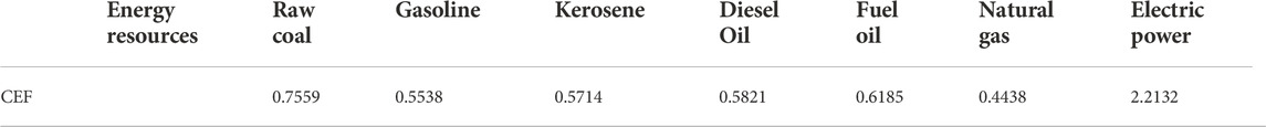
TABLE 1. Carbon emissions factors of various energy resources.

The panel unit root test and panel co-integration test

We first test the stationarity of output ($gd{p}_{i,t}$) and CO₂ emissions. For comparison, we use both the traditional IPS linear unit root test (Kim et al., 2003) and the nonlinear unit root test (CPLS test for short) proposed by Cerrato et al. (2009). The CPLS test can be carried out according to the procedure shown by Eqs. 2–8. These panel unit root test results are tabulated in Table 2, which shows that both carbon emissions and output of the logistics industry are $I\left(1\right)$ processes regardless of which forms are specified in testing models. Considering the low power of the traditional linear test, we turn to test whether there exists nonlinear co-integration between output ($gd{p}_{i,t}$) and CO₂ emissions. To do so, we first estimate the panel regression model, and then obtain residuals ${\widehat{u}}_{1i,t}$ and ${\widehat{u}}_{2i,t}$, as shown in Table 2.

TABLE 2

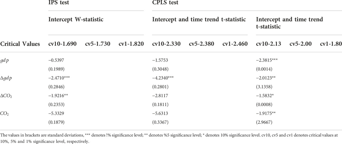
TABLE 2. Linear and nonlinear unit root tests.

Closed in parentheses beneath estimated coefficients in Table 2 are their companion t-statistics. We collect the residuals obtained from panel regression equations and implement a nonlinear co-integration test based on Eq. 8 and the linear co-integration test proposed by Pedroni (1999). These tests indicate a statistically significant cross-section dependence [measured by the CD statistic, (Pesaran, 2004)]. Indeed, the CD statistic of the CO₂ emissions (after being taken logarithm) is 90.286 (the companion p-value is 0.000); The CD statistic for the logarithm of output is 94.252 (the companion p-value is 0.000). In the presence of cross-section dependence, the bootstrap algorithm should be used to obtain the p values associated with the two test statistics, which are shown in Table 3.

TABLE 3

TABLE 3. Panel co-integration test results.

Although the IPS test shows that there is no co-integration relationship between CO₂ emissions and output of the logistics industry, the CPLS test shows the presence of co-integration between these two series. We estimate the nonlinear panel error correction model expressed by Eq. 10 allowing for nonlinear co-integration. Before estimating the PSTRVEC model, we estimate an appropriate linear model and perform linearity diagnosis first. The optimal lag orders of linear models are selected according to the AIC criterion, and parameter estimates are shown as follows:

$\Delta gdp={0.0827-0.0467}^{***}{\mathrm{e}\mathrm{c}}_{i1,t-1}+{0.3323}^{***}\Delta {\mathrm{g}\mathrm{d}\mathrm{p}}_{i,t-1}\left(0.0092\right)\left(0.0299\right){-0.0223}^{***}\Delta {\mathrm{C}\mathrm{O}}_{2i,t-1}$

$\left(0.0149\right)$

$\Delta C{O}_{2i,t}={0.1227-0.7007}^{***}{\mathrm{e}\mathrm{c}}_{2i,t-1}-0.0721\Delta {\mathrm{C}\mathrm{O}}_{2i,t-1}\left(0.1419\right)\left(0.0513\right)-0.1154\Delta {\mathrm{g}\mathrm{d}\mathrm{p}}_{i,t-1}\left(0.2347\right)$

*** denotes significance at 1% level, ** denotes significant level at 5%, * denotes significance at 10% level. The values in brackets are standard deviations.

The coefficients associated with error correction terms have correct signs in both equations and are statistically significant. Their negative coefficients indicate that a reverse adjustment dynamics exits between output growth and CO₂ emissions growth in the logistics sector. when they converge to the long-term equilibrium. Furthermore, other coefficients are statistically significant and have the expected signs.

Results of linearity tests

Although the linear models can achieve expected estimates to a certain extent, we test the linearity underlying the regression models in Eq. 12 yet on the safe side. For $k=\mathrm{1,2,3}$, the lagged output growth, the lagged CO₂ emissions growth and the lagged error correction terms are selected as transition variables alternatively, which can reflect the sources of all possible nonlinear relations between CO₂ emissions and output. For example, the lagged output growth as a transition variable can indicate that it is in which phase of business cycle that the non-linear relationship has happened between variables considered; If the lagged error correction term is used as a transition variable, the nonlinear relationship between CO₂ emissions growth and output growth depends on the degree of deviation from the long-term equilibrium level. If the lagged CO₂ emissions growth is used as a transition variable, the nonlinear dynamic relationship between CO₂ emissions growth and output growth depends on CO₂ emissions growth. All these results estimated are listed in Table 4.

TABLE 4

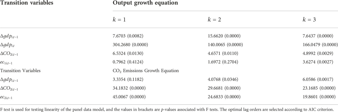
TABLE 4. Linearity test results.

As Table 4 shows, the null hypothesis of linearity can be rejected at the traditional significance level for both the output growth equation and the CO₂ emissions growth equation. As many studies show, there may be many reasons for the nonlinearity between output growth and CO₂ emissions growth. Specifically, identified nonlinearity arises mainly from output growth (i.e. different phases of the economic cycle). However, in CO₂ emissions growth equation, the nonlinear relationship is mainly caused by CO₂ emissions growth. Considering that the nonlinear relationship in different equations attributes to different transition variables, we choose output growth and CO₂ emissions growth as the transition variables in two equations respectively, and implement a series of $F$ tests proposed by Teräsvirta (1994) to select a specific form of the transition function. The $F$ test statistics are reported in Table 5 below.

TABLE 5

TABLE 5. Choice of transition functions.

The estimates of the panel smooth transition vector error correction model

Table 5 shows that among all F tests, the companion p-value of $F_1$ is the smallest. According to the inference rule proposed by Teräsvirta (1994), the logistic function is the most appropriate candidate. Further, we move on estimating the PSTRVEC model. Considering the possible cross-section correlation in panel data, we use the iterative generalized nonlinear least squares method to estimate the PSTRVEC model. The optimal lag orders of the model are selected by the AIC criterion. Table 6 reports our results.

TABLE 6

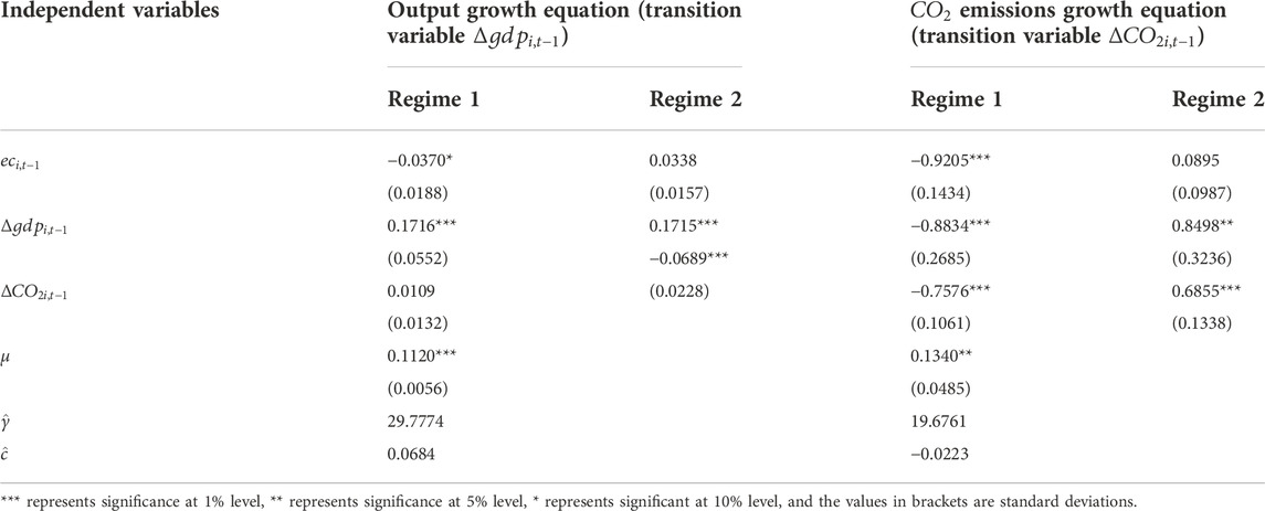
TABLE 6. Estimated Parameters of the PSTRVEC model.

As analyzed by the previous subsection, the relationship between output growth and CO₂ emissions growth varies over different phases of business cycle. Hence, it is reasonable to apply the estimated logistic transition function below,

$G\left(\Delta gd{p}_{i,t-1};\gamma ,c\right)={\left(1+\exp \left(-29.7774\left(\Delta gd{p}_{i,t-1}-0.0684\right)\right)\right)}^{-1},$

to two PSTRVEC equations, and estimated results are shown in Table 7.

TABLE 7

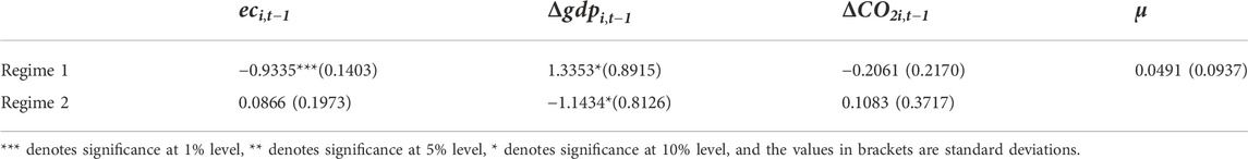
TABLE 7. Empirical results of CO₂ emissions equation when the transition variable is output growth.

As discussed above, the regime shifts of the PSTRVEC model are captured by transition function $G\left(s_{i,t};\gamma ,c\right)$, where the parameter $\gamma$ determines the speed of switching from an extreme to another, while the positional parameter $c$ determines the location of the midpoint of transition. In CO₂ emissions growth equation, the estimated positional parameter $\widehat{c}=-0.0223$ is very close to 0, indicating that the lowest regime in the estimated PSTRVEC model corresponds to the negative growth rate of CO₂ emissions in the logistics industry, while the highest regime matches the positive growth rate of CO₂ emissions. In fact, when the growth rate of CO₂ emissions is less than −0.1728, the value of $G\left(s_{i,t};\gamma ,c\right)$ is less than 0.01; while when CO₂ emissions growth rate is greater than 0.2518, the function $G\left(s_{i,t};\gamma ,c\right)$ is greater than 0.99. The estimated parameter $\widehat{\gamma }=19.6761$ indicates a smooth transition between two extreme regimes, as shown in Figure 1. Similarly, the transition speed parameter in the output growth equation is 29.7774, indicating that switching between two extremes is relatively smooth. The transition midpoint (the estimated positional parameter) is 0.09526, indicating that the impacts of CO₂ emissions on output growth in the logistics sector are mainly concentrated in those states of higher output growth, as shown in Figure 2.

FIGURE 1

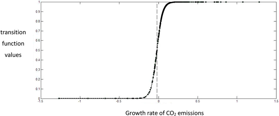
FIGURE 1. The scatter graph of the estimated transition function in the CO₂ emissions growth equation of the logistics sector.

FIGURE 2

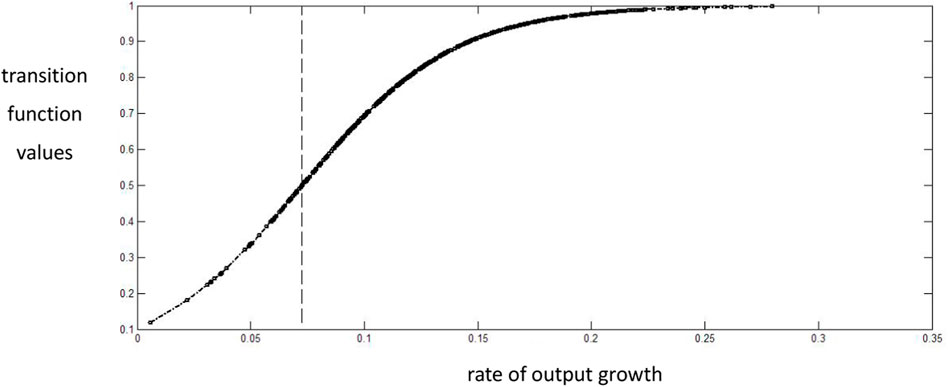
FIGURE 2. The scatter graph of the estimated transition function in the output growth equation.

We discuss the estimated coefficients of the PSTRVEC model Eq. 10. First, consider the output growth equation. When the economy is in a low output growth phase (i.e. when the output growth rate is lower than the mid-point value of the transition function, $G\left(s_{i,t};\gamma ,c\right)\approx 0$), the estimated coefficient of the error correction term is −0.0370, which is statistically significant. The negative coefficient of the error correction term means that the economy adjusts output in the opposite direction, once the output growth deviates from the long-term equilibrium level.

The mechanism of automatic stability is essential for the economy to escape from the low output growth phase. The estimated coefficient for CO₂ emissions growth in the logistics sector is 0.0109, which is statistically insignificant, implying that output growth increases as CO₂ emissions growth soars in the phase of the lower regime of output growth, although the evidence is (statistically) weak. When the economy is in the expansionary phase (i.e. when the output growth rate is higher than the midpoint value of regime transition function, $G\left(s_{i,t};\gamma ,c\right)\approx 1$), the estimated coefficient of the error correction term becomes −0.0032 (=−0.0370 + 0.0338), indicating that, in the higher economic growth phase, the mechanism of automatic stability is weakened and governmental policies for macroeconomic regulation are required. The estimated coefficient of CO₂ emissions growth is −0.058 (=0.0109–0.0689), which is statistically significant, indicating that CO₂ emissions impose a negative effect on output growth in the higher economic growth phase. Therefore, the Environmental Kuznets Curve (EKC) is proved to be true in China. In the initial phase of economic development, the output growth increases as CO₂ emissions soar. However, once output growth reaches a certain critical value, the reversed relationship can be discerned between output growth and CO₂ emissions growth.

Now consider the CO₂ emissions growth equation. When CO₂ emissions growth is at a low level, the estimated coefficient of the error correction term is equal to −0.9205, which is expected and statistically significant, indicating that the relationship between output growth and CO₂ emissions growth can be adjusted to a long-term equilibrium in the opposite direction. When CO₂ emissions growth is in a higher regime, the estimated coefficient of the error correction term is −0.831 (= −0.9205 + 0.0895), and its sign is as still expected. There exists a automatic stability mechanism between economic growth and CO₂ emissions growth such that the economy approaches to a long-term equilibrium, but at slower speed than in the lower regime of CO₂ emissions growth. This finding is very informative, implying the necessity of macroeconomic intervention once CO₂ emissions of the logistics industry are at a higher growth level. In the lower regime of CO₂ emissions growth, the estimated coefficient of output growth is −0.8834, which is statistically significant. In comparison, in the higher regime of CO₂ emissions growth, the estimated coefficient of output growth becomes −0.0336 (= −0.8834 + 0.8498). This finding indicates that, when CO₂ emissions growth is low, an increase in output growth might lead to a decrease in CO₂ emissions growth in the logistics sector, because output growth benefits CO₂ emissions reduction in the long term. However, if the CO₂ emissions growth is in a higher regime, the effect of output growth on CO₂ emissions reduction will be substantially reduced (shown by the fact that, when CO₂ emissions growth is in higher regime, the estimated coefficient is −0.0336).

When taking output growth $\Delta gd{p}_{i,t-1}$ as a transition variable and plugging it into the CO₂ emissions growth equation of the logistics sector, we can check how the output growth influences CO₂ emissions growth at different phases of the business cycle. In its lower phase, output growth influences CO₂ emissions growth positively, which is discerned from the positive coefficient of $\Delta gd{p}_{i,t-1}$ (1.3353), statistically significant at the significance level of 10%. The empirical finding indicates that output growth leads to an increase in demand for logistics services and an increase in CO₂ emissions simultaneously. However, when the output growth reaches a certain critical level, that is, when it is in a state of the higher regime, the pro-cyclical effect of CO₂ emissions growth in the logistics industry falls into a decline quickly, where the estimated coefficient of $\Delta gd{p}_{i,t-1}$ is only 0.1919 (1.3353–1.1434), statistically significant at the significance level of 10%. As results, accompanied with output growth, the logistics demand increases, but CO₂ emissions do not increase proportionally, which again shows that the Environmental Kuznets Curve holds in China.

Conclusion and implications

We use a panel dataset from 30 provinces and autonomous regions examining the dynamic relationship between CO₂ emissions growth and output growth in the logistics sector over the period 1995–2020. The panel co-integration test is implemented using a nonlinear smooth transition regression model. In the presence of nonlinear co-integration between two variables considered, the PSTRVEC model is specified and estimated. The PSTRVEC model can explore the nonlinear and asymmetric dynamic relationship between CO₂ emissions growth and output growth in the logistics sector. Several findings can be drawn from previous empirical analyses:

Firstly, only when the possible asymmetric relationship between CO₂ emissions growth and output growth of the logistics sector is considered, can we identify a nonlinear co-integration underlying the dynamic path approaching to their long-term equilibrium state. This empirical finding suggests that an emissions reduction policy will have an asymmetric impact on China’s output growth of the logistics industry.

The green logistics performance significantly impacts on output growth, but when output growth rounds the critical point, the impacts become positive. In the logistics sector, CO₂ emissions growth and output growth react differently to the deviation from the equilibrium path approaching their stable state in a different way. Hence, such an automatic stability process is very complex. This adjustment mechanism depends on which phases output growth and CO₂ emissions growth situate, respectively. In the higher regime of output growth, the automatic stability mechanism is weaker than in the lower phase of output growth. When CO₂ emissions growth in the logistics industry is at a higher level, the speed of adjustment to the equilibrium path is much slower. In addition, from a cross-sectional perspective, the relationship between CO₂ emissions growth and output growth in the logistics sector varies over geographical regions, depending on different levels of output growth. In developed regions, the adjustment speed of the equilibrium between CO₂ emissions growth and output growth is slower, and the response of the output growth rate to the equilibrium deviation from the equilibrium sate is lower than in less developed regions.

Secondly, as the nonlinear panel unit root test shows, the dynamic relationship between CO₂ emissions growth and output growth in the logistics industry is nonlinear. We are able to reject null hypothesis of a linear relationship when using three alternative transition variables. This finding suggests that researchers and policy makers must take into account the possible non-linear relationship between CO₂ emissions growth and output growth in the logistics industry. In the output growth equation, the null hypothesis of linearity is more convincingly rejected when the lagged output growth is used as a transition variable. In the CO₂ emissions growth equation, when the lagged CO₂ emissions growth is used as a transition variable, the null hypothesis of a linear relationship is more convincingly rejected. These findings suggest that the EKC hypothesis holds in China. In the lower phase of output growth, the CO₂ emissions growth of the logistics industry is pro-cyclical, while when the output growth rounds a critical point, the CO₂ emissions growth might become counter-cyclical.

Empirical results can appeal to policymakers to a more integrated and sustainable perspective, which gives higher priority to economic growth by reducing CO₂ emissions in the logistics sector. When exploring the relationship between CO₂ emissions growth and output growth in logistics sector, we find that the traditional linear relationship is not suitable. Our conclusions are important for policy authorities to consider potential asymmetries. The automatic stability mechanism of the dynamic relationship between CO₂ emissions and output growth in logistics industry is weaker during periods of higher output growth (or developed regions), indicating that China can conduct energy conservation policies to reduce CO₂ emissions in the logistics industry without worrying about damaging the long-term output growth. Energy conservation policies for CO₂ emissions reduction should not only limit the adverse effect on output growth in the short run, but also not harm output growth in long-term. In addition, we find that, when the initial output growth is relatively low, the output growth does not increase the CO₂ emissions of the logistics industry in the short term at all. However, in the long run, this is another story. In different output growth stages and different regions, the relationship between CO₂ emissions growth and output growth in the logistics industry reveals different patterns, which requires the government to consider regional gaps when designing energy saving and emission reduction policies. The Chinese government should focus on reducing CO₂ emissions of the logistics industry in economically developed areas, and formulate measures in favor of those developed areas and green logistics performance.

Data availability statement

The original contributions presented in the study are included in the article/Supplementary Material; further inquiries can be directed to the corresponding author.

Author contributions

In this article JW proposed the research ideas, formed the overall research goal, and completed the writing. Review and revision of the manuscript. He is the first to study the Nonlinear Dynamic Interrelationship between CO₂ Emissions and Output Growth in the Logistics Sector.

Funding

We acknowledge financial support from the research project “Research on Parameter dentification and Application of DSGE Models: Allowing for Indeterminacy” (Approval Number: 71863008) sponsored by National Natural Science Foundation of China, and from the research project “A Research on Bias Correction of Long Memory Semiparametric Estimators and Application of ARFIMA Models under High-Frequency Cantagion” (Approval Number: 72263010) sponsored by National Natural Science Foundation of China.

Conflict of interest

The author declares that the research was conducted in the absence of any commercial or financial relationships that could be construed as a potential conflict of interest.

Publisher’s note

All claims expressed in this article are solely those of the authors and do not necessarily represent those of their affiliated organizations, or those of the publisher, the editors and the reviewers. Any product that may be evaluated in this article, or claim that may be made by its manufacturer, is not guaranteed or endorsed by the publisher.

Footnotes

¹In Eq. 1, $y_{it}$ and $x_{it}$ are represented by $gd{p}_{it}$ and $C{O}_{2it}$ respectively, and then the dependent variable and independent variable are swapped to obtain two equations, and two residuals are estimated.

References

Abbes, S., and Bulteau, J. (2018). Growth in transport sector CO₂ emissions in Tunisia: An analysis using a bounds testing approach. Int. J. Glob. Energy Issues 41 (1-4), 176–197. doi:10.1504/ijgei.2018.092334

CrossRef Full Text | Google Scholar

Adebayo, T. S., Awosusi, A. A., Kirikkaleli, D., Akinsola, G. D., and Mwamba, M. N. (2021). Can CO₂ emissions and energy consumption determine the economic performance of South Korea? A time series analysis. Environ. Sci. Pollut. Res. 28 (29), 38969–38984. doi:10.1007/s11356-021-13498-1

PubMed Abstract | CrossRef Full Text | Google Scholar

Alinaghian, M., and Goli, A. (2017). Location, allocation and routing of temporary health centers in rural areas in crisis, solved by improved harmony search algorithm. Int. J. Comput. Intell. Syst. 10, 894–913. doi:10.2991/ijcis.2017.10.1.60

CrossRef Full Text | Google Scholar

Arouri, M. E., Youssef, A., M’henni, H., and Rault, C. (2012). Energy consumption, economic growth and CO₂ emissions in Middle East and North african countries. Energy Policy 45, 342–349. doi:10.1016/j.enpol.2012.02.042

CrossRef Full Text | Google Scholar

Awan, A., Alnour, M., Jahanger, A., and Onwe, J. C. (2022). Do technological innovation and urbanization mitigate carbon dioxide emissions from the transport sector? Technol. Soc. 71, 102128. doi:10.1016/j.techsoc.2022.102128

CrossRef Full Text | Google Scholar

Aydin, C., Aydin, H., and Altinok, H. (2022). Does the level of energy intensity matter in the effect of logistic performance on the environmental pollution of OBOR countries? Evidence from PSTR analysis. J. Environ. Plan. Manag., 1–19. doi:10.1080/09640568.2022.2030685

CrossRef Full Text | Google Scholar

Baek, J., and Kim, H. S. (2013). Is economic growth good or bad for the environment? Empirical evidence from Korea. Energy Econ. 36, 744–749. doi:10.1016/j.eneco.2012.11.020

CrossRef Full Text | Google Scholar

Cerrato, M., de Peretti, C., Larsson, R., and Sarantis, N. (2009). A nonlinear panel unit root test under cross section dependence, working papers 2009_28. Glasgow, United Kingdom: Department of Economics, University of Glasgow.

Google Scholar

Choi, E., Heshmati, A., and Yongsung, C. (2010). An empirical study of the relationships between CO₂ emissions, economic growth and openness. IZA Discussion Paper No. 5304 SSRN Available at: https://ssrn.com/abstract=1708750. doi:10.2139/ssrn.1708750

CrossRef Full Text | Google Scholar

Fleisher, B. M., and Chen, J. (1997). The coast-noncoast income gap, productivity and regional economic policy in China. J. Comp. Econ. 25 (2), 220–236. doi:10.1006/jcec.1997.1462

CrossRef Full Text | Google Scholar

Goli, A., Khademi-Zare, H., Tavakkoli-Moghaddam, R., Sadeghieh, A., Sasanian, M., and Kordestanizadeh, R. M. (2021). An integrated approach based on artificial intelligence and novel meta-heuristic algorithms to predict demand for dairy products: A case study. Netw. Comput. neural Syst. 32 (1), 1–35. doi:10.1080/0954898x.2020.1849841

PubMed Abstract | CrossRef Full Text | Google Scholar

Gonzalez, A., Teräsvirta, T., and Dijk, D. (2005). Panel smooth transition regression model. Sydney, NSW: Quantitative Finance Research Centre, University of Technology.

Google Scholar

Hansen, B. (1999). Threshold effects in non-dynamic panels: Estimation, testing and inference. J. Econ. 93 (2), 345–368. doi:10.1016/s0304-4076(99)00025-1

CrossRef Full Text | Google Scholar

Hassan, S. T., Khan, D., Zhu, B., and Batool, B. (2022). Is public service transportation increase environmental contamination in China? The role of nuclear energy consumption and technological change. Energy 238, 121890. doi:10.1016/j.energy.2021.121890

CrossRef Full Text | Google Scholar

IPCC (2006). “Summary for policymakers,” in Climate change: The physical science basis. Contribution of working group I to the fifth assessment report of the intergovernmental panel on climate change [stocker, T.F., D. Qin, G.-K. Plattner, M.

Google Scholar

Jing, A. H. Y., and Ab-Rahim, R. (2020). Information and communication technology (ICT) and economic growth in ASEAN-5 countries. J. Public Adm. Governance 10 (2), 2033. doi:10.5296/jpag.v10i2.16589

CrossRef Full Text | Google Scholar

Kapetanios, G., Shin, Y., and Snell, A. (2003). Testing for a unit root in the nonlinear STAR framework. J. Econ. 112, 359–379. doi:10.1016/s0304-4076(02)00202-6

CrossRef Full Text | Google Scholar

Kapetanios, G., Shin, Y., and Snell, A. (2006). Testing for cointegration in nonlinear smooth transition error correction models. Econom. Theory 22 (2), 279–303.

CrossRef Full Text | Google Scholar

Khan, M., and Eggoh, J. (2021). Investigating the direct and indirect linkages between economic development and CO₂ emissions: A PSTR analysis. Environ. Sci. Pollut. Res. 28 (8), 10039–10052. doi:10.1007/s11356-020-11468-7

PubMed Abstract | CrossRef Full Text | Google Scholar

Kim, T.-H., Pfaffenzeller, N. E. S., Rayner, T., and Newbold, P. (2003). Testing for linear trend with application to relative primary commodity prices. J. Time Ser. Anal. 24, 539–551.

CrossRef Full Text | Google Scholar

Li, H., and Ya, K. (2012). Research on the relationship between Industrial carbon emission and economic development in China. Macroeconomics (11), 46–52.

Google Scholar

Li, X., Sohail, S., Majeed, M. T., and Ahmad, W. (2021). Green logistics, economic growth, and environmental quality: Evidence from one belt and road initiative economies. Environ. Sci. Pollut. Res. 28 (24), 30664–30674. doi:10.1007/s11356-021-12839-4

PubMed Abstract | CrossRef Full Text | Google Scholar

Liu, C., Ji, W., AbouRizk, S. M., and Siu, M. F. (2019). Equipment logistics performance measurement using data-driven social network analysis. J. Constr. Eng. Manag. 145 (5), 04019033. doi:10.1061/(asce)co.1943-7862.0001659

CrossRef Full Text | Google Scholar

Liu, H., Yang, R., Wu, D., and Zhou, Z. (2021). Green productivity growth and competition analysis of road transportation at the provincial level employing Global Malmquist-Luenberger Index approach. J. Clean. Prod. 279, 123677. doi:10.1016/j.jclepro.2020.123677

CrossRef Full Text | Google Scholar

Lu, H. (2000). An analysis on China’s economy development and on state space model of environment —take air pollution as an example. J. Finance Econ. (10), 53–59.

Google Scholar

Lu, Q., Liu, H., Yang, D., and Liu, H. (2019). Effects of urbanization on freight transport carbon emissions in China: Common characteristics and regional disparity. J. Clean. Prod. 211, 481–489. doi:10.1016/j.jclepro.2018.11.182

CrossRef Full Text | Google Scholar

Luukkonen, R., Saikkonen, P., and Teräsvirta, T. (1988). Testing linearity against smooth transition autoregressive models. Biometrika 75, 491–499. doi:10.1093/biomet/75.3.491

CrossRef Full Text | Google Scholar

Maki, D. (2010). An alternative procedure to test for cointegration in STAR models. Math. Comput. Simul. 80, 999–1006. doi:10.1016/j.matcom.2009.12.003

CrossRef Full Text | Google Scholar

Muhammad, B. (2019). Energy consumption, CO₂ emissions and economic growth in developed, emerging and Middle East and North Africa countries. Energy 179, 232–245. doi:10.1016/j.energy.2019.03.126

CrossRef Full Text | Google Scholar

Omay, T., and Kan, E. Ö. (2010). Re-examining the threshold effects in the inflation–growth nexus with cross-sectionally dependent non-linear panel: Evidence from six industrialized economies. Econ. Model. 27 (5), 996–1005. doi:10.1016/j.econmod.2010.04.011

CrossRef Full Text | Google Scholar

Pao, H-T., and Tsai, C-M. (2010). CO2 emissions, energy consumption and economic growth in BRIC countries. Energy Policy 38, 7850–7860. doi:10.1016/j.enpol.2010.08.045

CrossRef Full Text | Google Scholar

Pedroni, P. (1999). Critical values for cointegration tests in heterogeneous panels with multiple regressors. Oxf. Bull. Econ. Stat. 61, 653–670. doi:10.1111/1468-0084.61.s1.14

CrossRef Full Text | Google Scholar

Pesaran, M. H. (2007). A simple panel unit root test in the presence of cross-section dependence. J. Appl. Econ. Chichester. Engl. 22 (2), 265–312. doi:10.1002/jae.951

CrossRef Full Text | Google Scholar

Pesaran, M. H. (2004). “General diagnostic tests for cross-section dependence in panels,” in Cam-bridge working papers in economics 0435 (UK: University of Cambridge).

Google Scholar

Rahman, M. M., Saidi, K., and Mbarek, M. B. (2020). Economic growth in South Asia: The role of CO2 emissions, population density and trade openness. Heliyon 6 (5), e03903. doi:10.1016/j.heliyon.2020.e03903

PubMed Abstract | CrossRef Full Text | Google Scholar

Sun, Y., Li, M., Zhang, M., Khan, H. S. U. D., Li, J., Sun H., Z., et al. (2021). A study on China’s economic growth, green energy technology, and carbon emissions based on the Kuznets curve (EKC). Environ. Sci. Pollut. Res. 28 (6), 7200–7211. doi:10.1007/s11356-020-11019-0

PubMed Abstract | CrossRef Full Text | Google Scholar

Teräsvirta, T. (1994). Specification, estimation, and evaluation of smooth transition autoregressive models. J. Am. Stat. Assoc. 89, 208–218. doi:10.2307/2291217

CrossRef Full Text | Google Scholar

Tirkolaee, E. B., Goli, A., Ghasemi, P., and Goodarzian, F. (2022). Designing a sustainable closed-loop supply chain network of face masks during the COVID-19 pandemic: Pareto-based algorithms. J. Clean. Prod. 333, 130056. doi:10.1016/j.jclepro.2021.130056

PubMed Abstract | CrossRef Full Text | Google Scholar

Uçar, N., and Omay, T. (2009). Testing for unit root in nonlinear heterogeneous panels. Econ. Lett. 104 (1), 5–8. doi:10.1016/j.econlet.2009.03.018

CrossRef Full Text | Google Scholar

Wang, K. M. (2012). Modelling the nonlinear relationship between CO2 emissions from oil and economic growthEmissions from Oil and Economic Growth. Econ. Model. 29, 1537–1547. doi:10.1016/j.econmod.2012.05.001

CrossRef Full Text | Google Scholar

Wang, L. (2021). Research on logistics carbon emissions under the coupling and coordination scenario of logistics industry and financial industry. Plos one 16 (12), e0261556. doi:10.1371/journal.pone.0261556

PubMed Abstract | CrossRef Full Text | Google Scholar

Wang, S. S., Zhou, D. Q., Zhou, P., and Wang, Q. W. (2011). CO₂Emissions, energy consumption and economic growth in China: A panel data analysis. Energy Policy 39, 4870–4875. doi:10.1016/j.enpol.2011.06.032

CrossRef Full Text | Google Scholar

Yuan, J. H., Kang, J. G., Zhao, C. H., and Hu, Z. G. (2008). Energy consumption and economic growth: Evidence from China at both aggregated and disaggregated levels. Energy Econ. 30 (6), 3077–3094. doi:10.1016/j.eneco.2008.03.007

CrossRef Full Text | Google Scholar

Zhao, X., and Hu, Y. (2013). Carbon market: Systematic risk and expectations of returns. J. Beijing Inst. Technol. 1, 5–11.

Google Scholar