Integration of shapley additive explanations with random forest model for quantitative precipitation estimation of mesoscale convective systems

Mesoscale convective cloud systems have a small horizontal scale and a short lifetime, which brings great challenges to quantitative precipitation estimation (QPE) by satellite remote sensing. Combining machine learning models and geostationary satellite spectral information is an effective method for the QPE of mesoscale convective cloud, while the interpretability of machine learning model outputs remains unclear. In this study, based on Himawari-8 data, high-density automatic weather station observations, and reanalysis data over the North China Plain, a random forest (RF) machine learning model of satellite-based QPE was established and verified. The interpretation of the output of the RF model of satellite-based QPE was further explored by using the Shapley Additive Explanations (SHAP) algorithm. Results showed that the correlation coefficient between the predicted and observed precipitation intensity of the RF model was .64, with a root-mean-square error of .27 mm/h. The importance ranking obtained by SHAP model is completely consistent with the outputs of random forest importance function. This SHAP method can display the importance ranking of global features with positive/negative contribution values (e.g., current precipitation, column water vapor/black body temperature, cloud base height), and can visualize the marginal contribution values of local features under interaction. Therefore, combining the RF and SHAP methods provides a valuable way to interpret the output of machine learning models for satellite-based QPE, as well as an important basis for the selection of input variables for satellite-based QPE.

1 Introduction

Precipitation plays an important role in the interaction of the hydrosphere, atmosphere and biosphere (Hobbs, 1989; Ren et al., 2021). A measurement of this quantity is needed not only for an understanding of atmospheric processes but also for a wide range of practical applications ranging from flood forecasting and water resource management to microwave communications. Its uneven spatial and temporal distribution often lead to extreme weather events such as rainstorms and drought, which have a serious impact on human activities (Futrell et al., 2005; Gao, 2022). Traditional ground-station observations of precipitation exhibited extremely high measurement accuracy on the point scale, but they cannot accurately reflect the precipitation on the regional scale owing to the sparse distribution and network density of stations. Ground-based radar observations can give the spatial and temporal distribution of precipitation within a 300-km radius range, but their spatial coverage cannot be scaled up to the global scale (Li et al., 2021a). With the development of meteorological satellites, satellite-based quantitative precipitation estimation (QPE) technology has been greatly conducted (Tang et al., 2015; Yang et al., 2018; Zheng et al., 2021). Because precipitation is a highly complex process, however, there is a non-linear relationship between the surface precipitation intensity and cloud-top optical physical variables, resulting in certain limitations in the precipitation estimation equation constructed with statistical methods (Atkinson and Tatnall, 1997).

Machine learning has been widely proved to be effective for solving such complicated problems that have non-linear correlation among their numerous inner components, to which it is extremely difficult to set up simple physical models by using ordinary mathematic analysis or statistical skills (El-Alfy and Mohammed, 2020). Therefore, machine learning algorithms such as random forests have the advantages in satellite-based QPE (Li et al., 2021b; Lao et al., 2021; Lao et al., 2021). However, most of their working processes are in a black box state, extremely complex, lack transparency, and are often difficult to interpret and fully understand. (Barredo Arrieta et al., 2019; Vilone and Longo, 2020). Currently, most studies set out to improve the accuracy of machine learning models for QPE and ignore the interpretation of the output of the machine learning model and the interaction between input variables (Bochenek and Ustrnul, 2022). In general, the complexity of a random forest is proportional to the number of training samples and decision trees. The deeper the decision tree, the more leaf nodes, and the higher the complexity of the random forest. However, with the increase in the complexity of the model, it has become a greater challenge to interpret the output of machine learning algorithms, and the interpretability of machine learning is still an issue. Models trained through algorithms are treated as black boxes, seriously hampering the use of machine learning in certain areas. As an interpretable approach to artificial intelligence, the Shapley Additive Explanations (SHAP) algorithms are defined as arbitrary interpreted approximations of the original model and are compatible with several types of machine learning algorithm (Pathy, et al., 2020; Ning et al., 2022). Machine learning algorithms used in combination with SHAP include random forest (RF) (Kim and Kim, 2022), extreme gradient enhancement algorithm (XGBoost) (Min, et al., 2022) and gradient enhanced decision tree (LightGBM) (Wen et al., 2021), etc.

In recent years, many studies have begun to use SHAP models to optimize machine learning models and interpret their output results (Bi et al., 2020; Ning et al., 2022). Covering the fields of clinical medicine (Wang et al., 2021), finance (Pérez-Castrillo and Sun, 2022), structural engineering (Mangalathu et al., 2020) and the environment (Tang et al., 2022). For instance, based on the RF algorithm and SHAP model, (Li et al., 2021a) analyzed the temporal and spatial variations of selected key factors affecting PM_2.5 (fine particulate matter) in Zhejiang Province, China. The results showed that the factors influencing PM_2.5 varied greatly during the study period, but the Shapley values indicated that their relative importance was consistent. Shapley values provide a valuable means for identifying regional differences in key factors affecting atmospheric PM_2.5 values and provide a reliable reference for pollution control strategies (Li et al., 2021b). All these previous studies demonstrate that SHAP, as an emerging artificial intelligence interpretable model, is increasingly being applied to different algorithms and fields, its reliability and practicality are being gradually tested, and its deep logic and significance are worthy of further study.

At present, few scientists in the field of meteorology, either in China or internationally, have combined SHAP models to analyze the influence of the output of machine learning models on feature dependence. Mesoscale convective systems (MCSs) are one of the most impactful weather phenomena on Earth (Chen et al., 2020). The small horizontal range and short life history of MCSs pose a great challenge to precipitation prediction. MCSs are defined as convective systems with contiguous area extends ≥100 km in at least one horizontal direction (Gray, 2011). More importantly, MCSs contribute to warm-season precipitation, both in the tropics and mid-latitude regions (Nesbitt et al., 2006; Rasmussen et al., 2016). Accompanied with MCSs, strong weather phenomena, such as strong thunderstorms, gales, rainstorms, hail, etc., often occurred (Parker et al., 2000; Johnson et al., 2021; Gao, 2022). Apparently, the MCSs with heavy precipitation were caused by even more complicated environment, which is worthy of examination from the machine learning perspective. To date, spectral information based on geostationary satellites combined with machine learning (ML) models is an effective way to predict precipitation in MCSs (Kühnlein et al., 2014; Sanò et al., 2015; Min et al., 2019; Gaur et al., 2020), while there have been no reports on predicting mesoscale convective cloud precipitation in combination with SHAP models.

Therefore, an attempt was made to explore the QPE issue of mesoscale convection by combining SHAP with the random forest algorithm. In particular, it is necessary to use interpretable models such as SHAP to improve the transparency of the model and explore the specific effects of global and local features on the results to support more accurate QPE. This paper takes MCSs in eastern China during April-Jun of 2016 as a case study (Figure 1). By using ground-based high-density automatic station data, European Centre for Medium-Range Weather Forecasting (ECMWF) reanalysis data, and Himawari-8 satellite data, 15 variables, such as relative humidity (RH), current precipitation, and black body temperature (tbb), were used as input factors to build an RF model of satellite-based QPE. The SHAP model was introduced to elaborate on the global and local interpretability, with our objective is to explore: 1) the order of importance and dependencies of global features; 2) under their interaction, the influence of two local features and individual local features on the prediction results; and 3) the interpretability of random forest models to provide scientific reference for more accurate QPE.

FIGURE 1

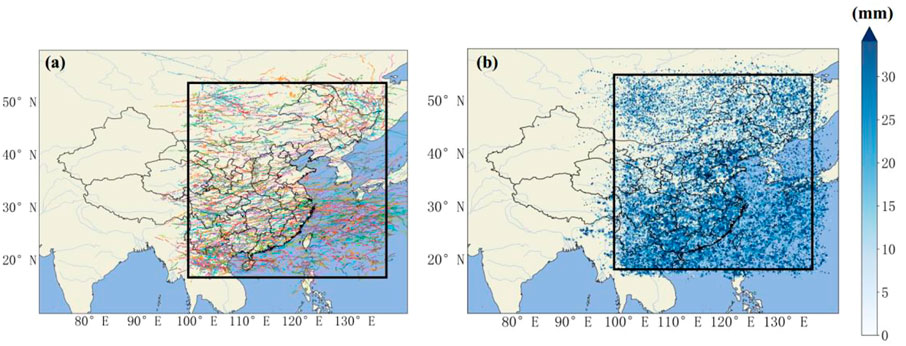
FIGURE 1. Object of study: (A) the trajectory of convective clouds studied; (B) maximum instantaneous precipitation in the MCS (mm).

2 Material and methodology

2.1 Material

The Himawari-8 meteorological satellite is one of the Himawari series of satellites designed and manufactured by the Japan Aerospace Exploration Agency, and is a new generation of meteorological satellites launched by Japan on 7 October 2014. The Himawari-8 data have 16 observation bands, distributed from the visible, to near-infrared, to thermal infrared wavelengths.

Himawari-8 carries an Advanced Himawari Imager (AHI) scanning five areas: Full Disk (images of the whole Earth as seen from the satellite), the Japan Area (Regions 1 and 2), the Target Area (Region 3) and two Landmark Areas (Regions 4 and 5). While the scan ranges for Full Disk and the Japan Area will be preliminarily fixed, those of the Target Area and Landmark Areas will be flexible to enable prompt reaction to meteorological conditions. At the beginning of Himawari-8’s operation, Landmark Area data will be used only for navigation, and are not intended for use as satellite products. No matter what shooting mode, the time resolution can reach at least 10 min. The time resolution of the mode of shooting Landmark Areas can reach .5 min. The spatial resolution is up to 500 m, and cloud parameter information can be inverted from Himawari-8 data (links to data: https://www.eorc.jaxa.jp/ptree/).

The European Centre for Medium-Range Weather Forecasting (ECMWF, an international organization supported by 34 countries, is currently the world’s leading international weather forecasting research and business organization. It was officially established in 1975 and then expanded its operations in June 1979 to real-time medium-term weather forecasts. ERA5 is the ECMWF’s latest (fifth generation) atmospheric reanalysis dataset, covering the Earth on a 30-km grid and using 137 horizontally resolved atmospheric layers from the surface to an altitude of 80 km, with a horizontal resolution of .25 × 0.25 (links to data: https://cds.climate.copernicus.eu/cdsapp#!/home).

The precipitation dataset was obtained from the hourly observation data of China’s ground-based, high-density network of automatic weather stations. These stations are an important means to fill the gaps not covered by spaceborne meteorological detection data, and can be used for all-weather on-site monitoring of more than a dozen meteorological elements such as wind speed, wind direction, rainfall, air temperature, and air humidity.

2.2 Methodology

The overall design of the study is illustrated in Figure 2. The specific details are explained in the following subsections.

FIGURE 2

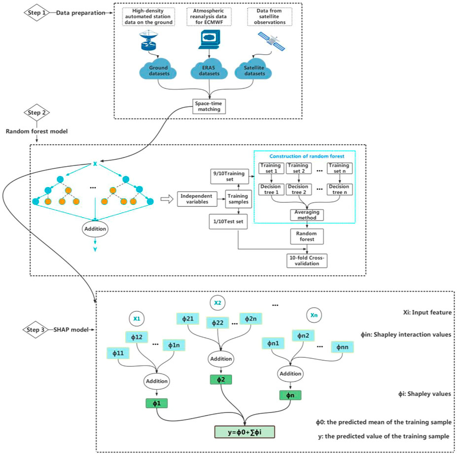
FIGURE 2. Research roadmap.

2.2.1 Pre-processing of data and input variables

In this paper, the geographic and precipitation information of high-density automatic stations with 1-h resolution, HW8/AHI observation data and ERA5 reanalysis data are selected as RF model inputs. According to the geographic location and time information of high-density automatic stations, the ERA5 and satellite data were matched with data from the station by using the bilinear interpolation method. The fused data, such as tbb, RH, and precipitation in the previous hour, were used as input variables to train a random forest model (see Table 1).

TABLE 1

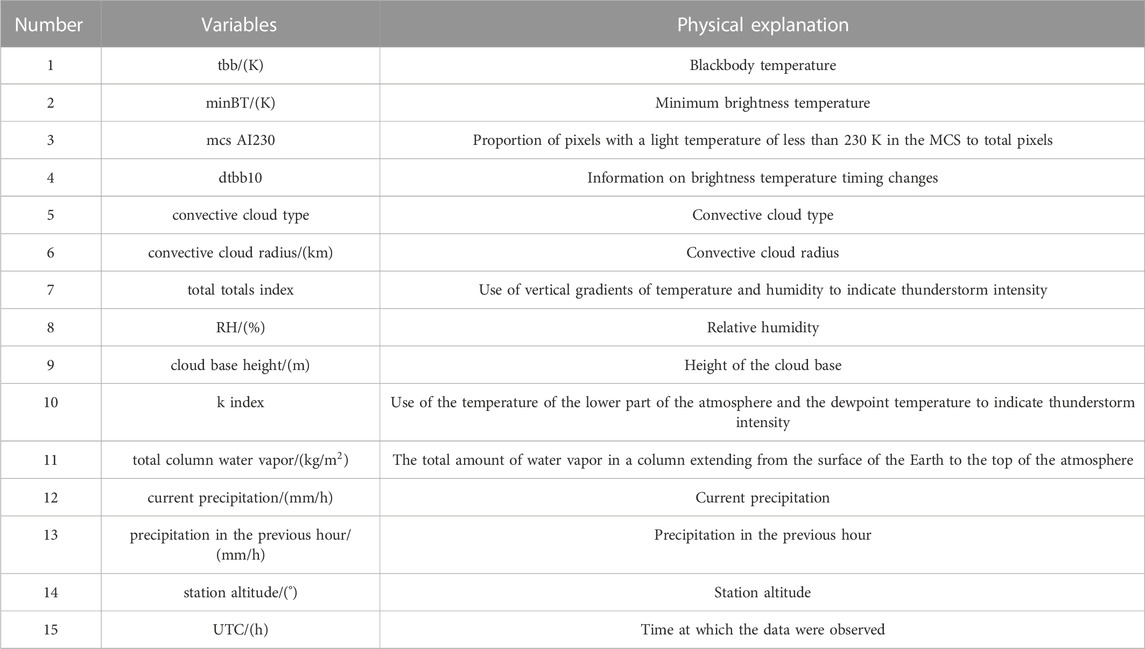
TABLE 1. Input variables for the random forest model.

2.2.2 Random forest model

Random forest () is a machine learning algorithm (Breiman, 2001; Ziegler and Koenig, 2014). The superiority of the random forests approach is reflected in i) its high level of accuracy compared to all other current algorithms and its ability to run efficiently on large data sets; ii) its ability to process input samples with high-dimensional features without the need for dimensionality reduction; and iii) its ability to assess the importance of individual features in classification issues. Furthermore, it can also obtain good results for the default value problem, is increasingly being used in various industries, and is widely regarded as one of the best algorithms at present (Genuer et al., 2010).

This paper uses Random Forest Regressor packets in the Python language to construct a random forest model to predict the precipitation intensity for the next hour. The independent variables of the model input are the real-time data of this time, including current precipitation, tbb, and RH, etc., as shown in Table 1, and the dependent variable is the log value of the precipitation rate of the next hour [lg (Rain Rate)]. For the constructed data set, the sites in the MCS domain of several times are randomly extracted from it, so that they do not participate in the modeling process at all. They are used as the final verification set of the model, and the rest of the data are training sets. The training set is input into the RF model for grid parameter adjustment based on cross validation, so as to construct the precipitation prediction model with the highest accuracy. Finally, the order of importance of modeling variables is given to obtain the characteristic analysis with physical significance. The specific parameters are set as follows: the number of branches of the decision tree is 250; the maximum depth of the tree is 30; the minimum number of samples required at the leaf node is two; the minimum number of samples for each division is two when dividing the nodes according to attributes; and the number of samples for features to consider when finding the best split on each node is 80.

Finally, the training set is input into the RF model for grid parameter adjustment based on 10-fold cross-validation (CV), so as to construct the precipitation prediction model with the highest accuracy. Finally, the order of importance of modeling variables is given to obtain the characteristic analysis with physical significance. In the 10-fold CV, the training set is divided into 10 sample subsets, and 9/10 of the samples are randomly selected as the training dataset to establish a random forest model with each instance of training, and the remaining 1/10 samples are used as the test dataset for verification of the prediction accuracy of the established random forest model. The process is repeated until all the samples have been predicted at least once. The complexity of 10-fold CV calculations is relatively high, but the data are fully utilized, which has obvious advantages for the case of a relatively small dataset, and can improve the accuracy of model prediction. Finally, the model is judged by the correlation coefficient (r) and root-mean-square error (RMSE), in which r represents the correlation between the predicted value of the model and the true value, and the RMSE is the sum of squares of the deviation of the predicted value from the true value divided by the number of predictions, and then taking the square root of the value of the result. The higher the r value, the smaller the RMSE value and the higher the model accuracy (Kuhnlein et al., 2014).

3.3 SHAP model

3.3.1 Definition and implementation of SHAP model

SHAP is a game theory method used to interpret the output of any machine learning model. SHAP interprets the Shapley value as an additive feature attribution method that interprets the predicted values of the model as the sum of the attributed values of each input feature, thus achieving an arbitrary explanatory approximation of the original model. Referring to previous studies (Shapley, 1952; Roth and Shapley, 1991; Kuhnlein et al., 2014), the principles of implementation for SHAP can be briefly described as follows: Each input feature has a corresponding attribution value—namely, Shapley values (${\mathrm{\varphi }}_{\mathrm{i}}$)—and then Shapley interaction values (${\mathrm{\varphi }}_{\mathrm{i}\mathrm{j}}$) are interaction attribution values between two features that capture the effect of paired interactions. Its connection to the attribution value is that the attribution value that each feature has is determined by the sum of a series of interactive attribution values ($\sum {\mathrm{\varphi }}_{\mathrm{i}\mathrm{j}}={\mathrm{\varphi }}_{\mathrm{i}}$), so that the predicted value of the training sample can be expressed as the sum of the predicted mean and the total sample attribution value ($\mathrm{y}={\mathrm{\varphi }}_0+{\displaystyle \sum }_{\mathrm{i}=1}{\mathrm{\varphi }}_{\mathrm{i}}$ , where ${\mathrm{\varphi }}_0$ is the predicted mean of the training sample). When the model changes so that the marginal contribution value of the feature value increases or remains unchanged (regardless of other features), the attribution value also increases or remains unchanged.

In the SHAP plot, if the Shapley value is greater than 0, it indicates that the prediction is pushed higher, i.e., a positive contribution; and if the Shapley value is less than 0 it means the forecast is pushed lower, i.e., a negative contribution.

3.3.2 Classification in a SHAP diagram

SHAP can be classified according to different evaluation criteria, and this paper divides it into visual feature importance, realizing the clustering of samples and features, and interpreting the model output. When visualizing the sorting of feature importance, a simple plot (plot type = ‘bar’) or a bar plot is often used to reflect the importance of all features. When clustering samples and features (Lundberg et al., 2018), hierarchical clustering is achieved using shap. utils.hclust, i.e., a hierarchical nested clustering tree is created by calculating the similarity between data points in different categories. In feature clustering, by controlling the degree of redundancy, you can analyze features with a high degree of correlation. In sample clustering, the distribution intervals of high-quality samples can be visualized to some extent. When interpreting the model output, the summary plot or beeswarm plot is used to demonstrate the positive and negative effects of all features, and include the ranking of feature importance. A force plot or waterfall plot is used to demonstrate the influence of features on single or multiple samples. A dependence plot is used to explore the interaction between one or more pairs of features to obtain Shapley interaction values (Lundberg et al., 2020). This is a method of generalizing SHAP to higher-order interactions, enabling fast, precise, two-by-two interaction calculations that show whether the relationship between dependent variables and features is linear, monotonous, or more complex. Dependence plots tend to reveal interesting hidden relationships between features, which is the focus of this paper.

3.2.3 Advantages of the SHAP model

Currently, many of the methods used to interpret local predictions of machine learning models belong to the attribution of added features, such as LIME, DeepLIFT, and hierarchical correlation propagation. SHAP, on the other hand, can unify the interpretation prediction framework of the above methods. The advantages of the SHAP model can be broadly summarized as simplicity, visibility, reliability, and comprehensiveness. More specifically, SHAP is a “model explanation” package developed by Python, which can be used by users after installation. The SHAP model visualizes complex Shapley values, and the relationship between features and features or features and variables can be intuitively explored through analysis graphs. Shapley values are the only method of interpretation with solid theories, the main idea of which is the Shapley value, a method from cooperative game theory created by Shapley (1952) that can rigorously prove its reliability. SHAP has the ability to interpret both global and local features (Lundberg et al., 2020) while exploring overlooked physical laws based on interactions between features.

4 Results and discussions

4.1 Verification of the random forest model and ranking of feature importance

The RF model was verified by the 10-fold CV method, where the r of the training set was .92 and the RMSE was .14 mm/h. The r of the test set was .64 and the RMSE was .27 mm/h, which is more accurate for predicting the precipitation. A frequency scatter plot (logarithm) of the training set prediction results predicted by the random forest model and the precipitation data observed at the site is shown in Figures 3A frequency scatter plot (logarithm) of the test set prediction results versus the precipitation data observed at the site is shown in Figure 3B. From the color shading, which indicates the density distribution, it can be seen that a large amount of the precipitation observations and estimations are concentrated around 1:1 line, indicating that the algorithm has a high quantitative estimation ability for precipitation. However, due to the error of the dataset itself after the spatiotemporal matching, the accuracy of the model will be affected to some extent. Thus, in Figure 3A, B it is clear to see that the data have a certain inclination, a slope of less than 1, and there is a certain degree of underestimation in the model. The Python language provides an importance function that sorts the variables of the input model by importance, as shown in Figure 3C.

FIGURE 3

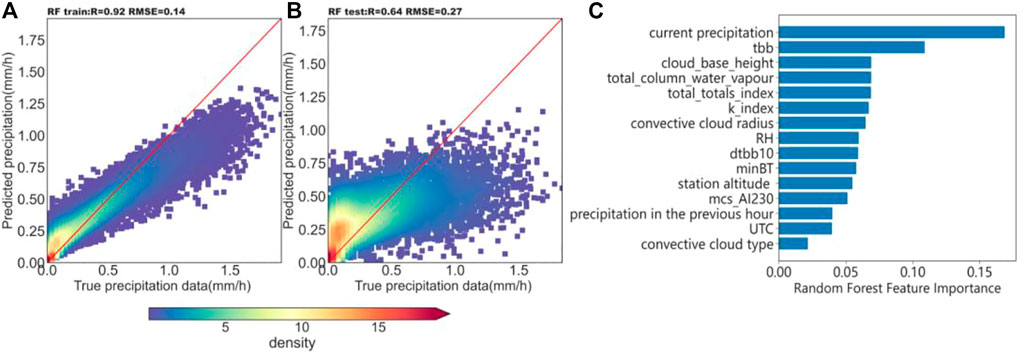
FIGURE 3. Scatter density plot of logarithmic values of predicted precipitation rates and measured precipitation data in the training set (A) and test set (B) for fusion parameter modeling, and (C) the ranking plot of the importance of features.

4.2 Interpretation of global features from the SHAP model

4.2.1 Ordering and influencing the importance of features

The global features are all the input variables of the RF model. In this paper, the order of global feature importance with positive and negative influences was sorted based on the output of the RF model using the summary plot (Figure 4). Color shading in Figure 4 indicates the size of the features, with red representing the larger values and blue the smaller values. The top-down ordering in the figure indicates that the feature importance is from high to low, and it can be known in Figure 3C, and the importance ranking obtained by the SHAP model is exactly the same as the result of the random forest importance function. In particular, Figure 4 can also exhibit the influence of a certain feature on the prediction in a certain interval segment based on the change of the Shapley values.

FIGURE 4

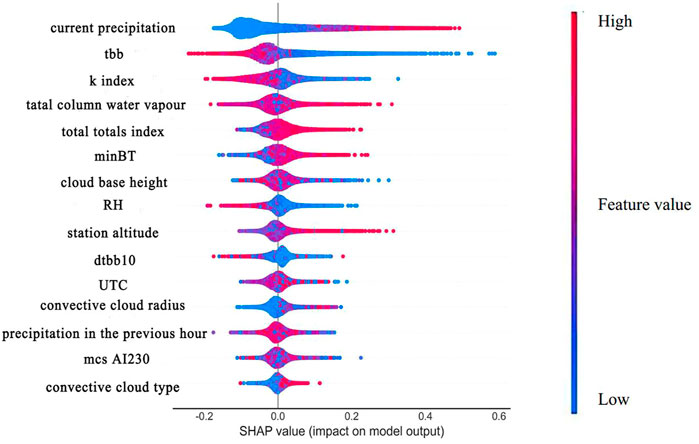
FIGURE 4. Summary plot of feature importance ranking and positive and negative influence in SHAP.

Taking current precipitation, which is the most important feature, as an example, the redder the color, the larger the value of current precipitation, and the corresponding Shapley value increases and is always greater than zero, i.e., the positive contribution to the prediction (overestimation) increases; and the bluer the color, the smaller the value of current precipitation, and the corresponding Shapley value gradually decreases from positive to negative, i.e., the contribution to the prediction changes from positive (overestimation) to negative (underestimation). Overlapping data points are scattered in the y-axis direction, e.g., the blue area of current precipitation is obviously more discrete on the y-axis than the red area, which indicates that the data contain a large number of samples with low values of current precipitation. This is highly consistent with the samples used for training. In the surface station observation data, the number of non-precipitation pixels was 493760, the number of precipitation pixels was 199119, and the number of non-precipitation samples was obviously more than that of precipitation samples.

Meanwhile, the values of current precipitation and mcs Al230 are positively proportional to the Shapley values, and the positive and negative effects are obvious. In addition, the values of tbb and cloud base height are inversely proportional to the Shapley values, and their positive and negative effects are also obvious. When the values of k index and total column water vapor increase, the Shapley value increases, which has an obvious positive effect. However, when these two values decrease, the Shapley value decreases less, suggesting that their negative effects are not obvious. The similarity of the relationship between different features and Shapley values can explain the similarity between features to some extent. This can be demonstrated in feature clustering.

4.2.2 Clustering of features and samples

Cluster analysis is an important unsupervised learning method whose importance as a tool for data analysis is widely recognized in various fields (Rui and Wunsch, 2005). The purpose of clustering is to look for “natural groupings” in a dataset—the so-called “clusters.” Put simply, it refers to the analysis process of grouping a collection of physical or abstract objects into classes consisting of similar objects. Clustering algorithms are not always effective, or even completely unreasonable, but there are multiple meaningful ways to divide them that are worth exploring.

Feature redundancy is measured in SHAP by model loss comparison using the shap. utils.hclust method and by training a RF model to predict the results of each pair of input features, which is used to build hierarchical clustering of features (Mahlstein and Knutti, 2010). Features of typical structured datasets are more accurate than those obtained from unsupervised methods such as correlation (Yogiraj and Ashish, 2016). The results of the computed clustering are passed to the bar chart, which visualizes both the feature redundancy structure and the feature importance. Suppose that the distances in a cluster are approximately scaled between 0 and 1, where 0 represents full redundancy among features and 1 means they are completely independent. By default, the shap. utils.hclust method only displays the clustering part of the distance <.5, and changing the value of the clustering cutoff can obtain different degrees of clustering, such as for clustering cutoff = .6, the clustering part of the distance <.6 is displayed. As shown in Figure 5A, when clustering cutoff = .5, only k index and total column water vapor are displayed with more than 50% redundancy. It can be said that the two are highly correlated, and there is a multicollinear problem of features, so they are the only features grouped in the bar chart. In the summary plot, we found similarities between the k index and the total column water vapor in their influence on the predictions, confirming our conjecture of the similarity of the two through feature clustering. From the physical perspective, the k index is a measure of the development potential of thunderstorms calculated based on the temperature of the lower part of the atmosphere and the dewpoint temperature. In addition to representing the rate of vertical decrease in temperature, it also contains the humidity conditions and saturation of the middle and lower layers of the atmosphere. The more abundant the water vapor at low altitude, the larger the k index value, and the more unstable the atmospheric stratification, the higher the probability of MCSs development (Ruoyun et al., 2021). Total column water vapor represents the total tower water vapor, which is the total amount of water vapor in a column that extends from the Earth’s surface to the top of the atmosphere. The three elements conducive to the occurrence and development of thunderstorms refer to unstable layer junctions, good low-altitude water vapor conditions and appropriate triggers (Colman, 1990; Ban et al., 2015). It can be seen that water vapor conditions play an important role in the occurrence of MCSs, thus confirming the high correlation between the characteristics of k index and total column water vapor. As shown in Figure 5B, when clustering cutoff = .7, the groupings of current precipitation and precipitation in the previous hour were added, as well as minBT and mcs Al230 after completing the first layer of clustering, and continued to complete the grouping of the second layer of clustering with convective cloud radius. This indicates that each group has more than 30% redundancy.

FIGURE 5

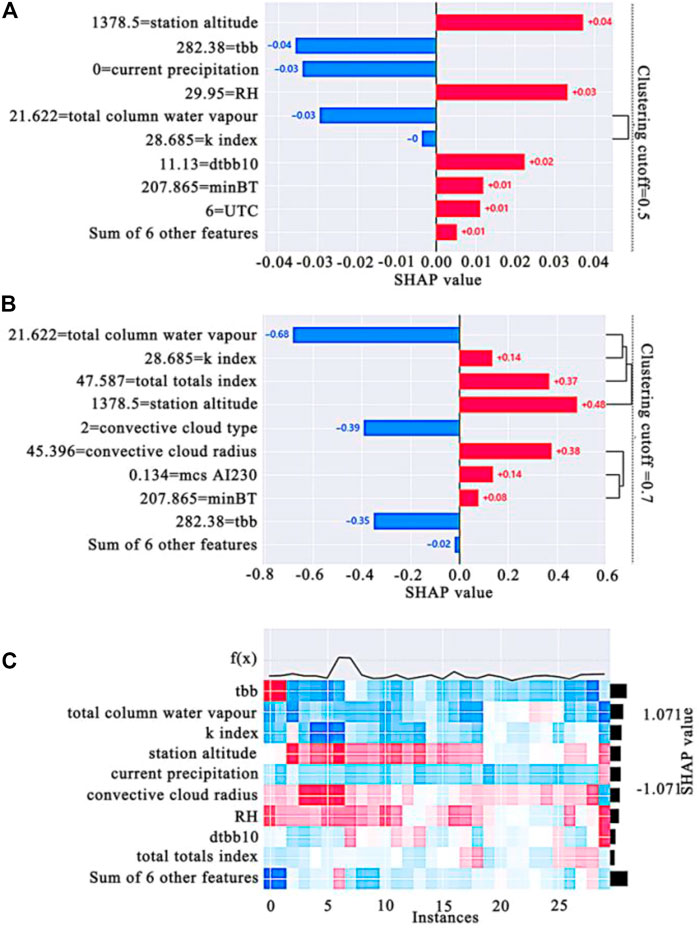
FIGURE 5. Feature clustering: (A) cluster distance <.5; (B) cluster distance <.7; and (C) sample cluster plots.

In addition to clustering features, we can also use shap. plots.heatmap to perform heat mapping analysis on samples. As shown in Figure 5C, the sample color patches are so evenly distributed because the dataset first undergoes a hierarchical clustering of shap. utils.hclust. In this plot, the numerical values of the x-axis represent the sample series, and the f(x) function plot above the x-axis is the sum of the Shapley values of all the features of each sample (the sum of the Shapley values of the sample dimension), representing the degree of deviation from the mean (the dotted line in the figure represents the mean). The left-hand y-axis is the feature name, the right-hand y-axis is the feature importance (the sum of the Shapley values of the feature dimensions), and the streak in the middle is the size of the Shapley value for each feature in each sample. It can be clearly seen that from the zero to fifth sample, the tbb color block shows a clear blue color, indicating that these five samples are greatly affected by the negative direction of tbb, and the sum f(x) of the sample Shapley value is also lower than the average line, which is unified. In a sense, the zero to fifth samples are high-quality samples when the study features tbb.

4.3 Interpretation of local features in SHAP models

Local features refer to some of the input variables of RF models, and we can interpret local features through analyzing the feature dependency and interaction. Interaction refers to the phenomenon whereby the difference in the amount of reaction between the levels of one variable changes with the different levels of other variables. The presence of interaction suggests that the effects of several variables studied at the same time are not independent. Shapley interaction values are interaction attribution values between two features that capture the effect of interactions in pairs, which can maintain consistency while explaining the interaction of individual predictions.

4.3.1 Understanding interactions with tbb

In the previous random forest feature importance ranking and SHAP’s supreme plot graph, tbb ranked second. Next, therefore, we attempt to understand the interaction with tbb.

Tbb is used to indicate the radiant temperature of a cloud-top black body and is closely related to the development of precipitation. If it is a strong convective weather development, the blackbody temperature is generally below −60°C; and the lower the blackbody temperature, the higher the cloud top, the more vigorous the convection, and the greater the potential for precipitation (Adler and Mack, 1984; Chen et al., 2007). Tbb ranks second in the order of feature importance of random forests, and has a clear negative correlation with Shapley values, so the role of tbb in precipitation prediction is further explored by combining feature dependency graphs with interactions. The following analysis is carried out with reference to existing studies (Wieland et al., 2020; Feng et al., 2021). In Figure 6A, tbb is the first feature and current precipitation is the second feature. It is found that when tbb > 230 K, the colors have a pronounced differentiation in the vertical direction. In this interval, when the current precipitation value is larger, the Shapley value of tbb is small, basically below zero, which has an underestimated effect on the QPE result, corresponding to the red data point. When the current precipitation value is small, the Shapley value of tbb is larger, basically located at or above zero, which has no impact on the QPE result or has an overestimated effect, corresponding to the blue data point. This shows that the interaction effect of current precipitation on tbb shows a clear negative correlation with the size of the Shapley value of tbb.

FIGURE 6

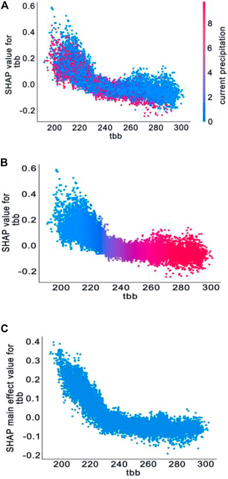
FIGURE 6. Characteristic-dependent plots of tbb (K): (A) feature dependency graph showing the interaction of current precipitation with tbb(K); (B) feature dependency graph that represents the comprehensive interaction of all the remaining input features on the tbb (K); (C) feature dependency graphs that eliminate interactions.

Figure 6B is a feature dependency graph of tbb that also shows the variance on the y-axis, and this is because there is an interaction of all other features, so the dependency graph diverges vertically. Figure 6C is a dependency plot that removes the interaction, and it can be clearly seen that after removing the interaction of other features, the vertical divergence of the data point distribution is weakened. It tends to fluctuate up and down in a certain concentration area. At the same time, all three graphs have an inflection point near the tbb value equal to 230 K. When the tbb value is less than 230 K, the slope is less than zero, and the absolute value is larger. When the tbb value is greater than 230 K, the absolute value of the slope decreases rapidly, even close to zero. This means that in the interval where the tbb value is less than about 230 K, the tbb is inversely correlated with its Shapley value and the rate of change is large, and the Shapley value increases rapidly with the decrease of the tbb value; that is, the overestimated effect on the QPE is rapidly enhanced, and the estimated precipitation probability is increased. In the interval where the tbb value is greater than 230 K, tbb is negatively correlated with its Shapley value and the rate of change decreases obviously, and the Shapley value hovers around −.1 with the increase of the tbb value; that is, it has a weak underestimated effect on the QPE, and the underestimated effect does not change much with the tbb, reducing the probability of estimated precipitation.

As can be seen in Figure 4, the red and blue colors are obviously layered near where the Shapley value is equal to zero, which means that it is close to the mean of tbb. Comparing the length of the red and blue bars, when the Shapley value is positive and the tbb value changes from the lowest value to the mean, the absolute value of the Shapley value changes greatly. When the Shapley value is negative and the tbb value changes from the highest value to the mean, the absolute value of the Shapley value change is smaller. That is, the inflection point of the image should appear near the Shapley value of zero, i.e., the tbb value in the feature dependency graph is near 230 K. According to existing studies, there is an obvious non-linear change between the blackbody temperature and the precipitation, and the two are negatively correlated within a certain temperature range. Some studies that have comprehensively considered the relationship between tbb and precipitation in different regions (Molinie and Jacobson, 2004) found that values of blackbody temperature prone to precipitation are concentrated between 210 K and 250 K, which is basically consistent with the conclusions observed from the SHAP plot.

4.3.2 Explaining the anomalous prediction of RH

Water vapor at low-level atmospheric layer accounts for a large proportion of the total atmospheric water vapor content of the whole layer, and the total amount of water vapor in the whole atmosphere is closely related to the ground humidity, which can reflect the amount of water vapor content of the whole atmosphere through the ground humidity (Brenner, 2004). Relative humidity at surface, hereinafter referred to as RH, is defined as the percentage of the ratio of the actual water vapor pressure (e) to saturated water vapor pressure (es) on the surface, which characterizes the saturation of water vapor in the atmosphere. As an important factor in regulating the balance of surface water and energy, the change of RH is closely related to precipitation and air temperature. The same approach as before is used with RH to make feature dependency plots (Figure 7A) and feature dependency plots after eliminating interactions (Figure 7B). Anomalous predictions occur approximately in the range where RH is less than 30%, at which point RH corresponding to a Shapley value greater than zero implies an overestimation of precipitation predictions, which is contrary to the experience of model predictions of no precipitation when the relative humidity is low (Lin et al., 2007; Todd et al., 2018). Therefore, this section attempts to provide a physical explanation for the occurrence of anomalous predictions at RH less than 30%.

FIGURE 7

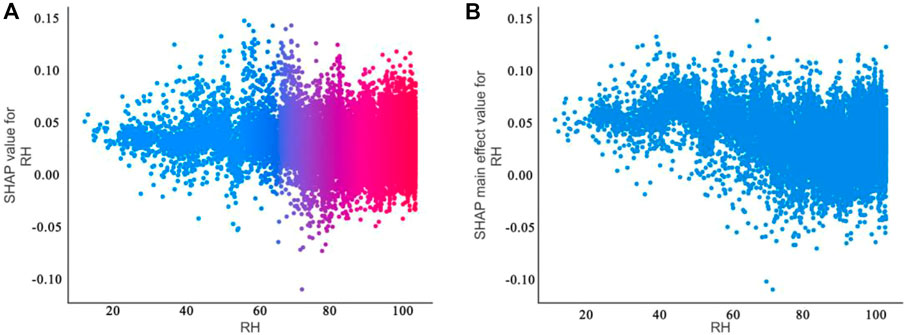
FIGURE 7. Characteristic-dependent plots of relative humidity (%): (A) feature dependency graph that represents the comprehensive interaction of all the remaining input features on the RH (%); (B) feature dependency graphs that eliminate interactions.

In addition, there are two more noteworthy points in the range where RH is greater than 80%. Firstly, in this interval, the upper and lower edges of the Shapley value distribution band show an obvious upward trend. This suggests that, to some extent, RH may be constraining the upper and lower limits of precipitable water. Secondly, the change in slope in the feature-dependency graph of the eliminated interaction is obviously greater than that in the plot when the interaction is not eliminated, which suggests that when RH is larger, the interaction of other features mitigates the effect of RH on precipitation prediction.

In the range of RH less than 30%, the Shapley value distribution band is almost horizontal, indicating that precipitation prediction is less affected by RH changes and there is almost no interaction effect of other factors. Therefore, it is speculated that in this area (31.7167°–43.3°N, 103.717°–128.183°E), when RH < 30%, the precipitation in the next moment is mainly from non-local water vapor. According to previous studies (Xu et al., 2020; Zheng et al., 2021; Yang et al., 2022), local water vapor comes from local surface evaporation and plant transpiration, and the starting height is the same as the surface height, which belongs to the relatively low layer of water vapor. Non-local water vapor comes from surface evaporation and plant transpiration in other places, and is transported horizontally and vertically to the local sky, which has a higher average altitude and belongs to the relatively high-rise water vapor. According to this, comparing the relative humidity and absolute humidity of different levels in the region for this period, if the relative humidity and absolute humidity values meet, the upper-layer water vapor is greater than the near-surface layer water vapor. To a certain extent, the source of precipitation can be characterized as non-local water vapor. Therefore, this paper uses the ground station data to extract the longitude, latitude and time corresponding to RH < 30%, matches the ERA5 reanalysis data of different levels of relative humidity and absolute humidity in this time and space, and uses 925 hPa to approximate the near-surface layer and 700 hPa to approximate the middle and upper layers. After averaging the time, the results present in Table 2 were obtained. It can be seen that the relative humidity of the 700 hPa level is obviously greater than the relative humidity of the 925 hPa level, and the absolute humidity of the two is smaller and the size is close, so it can be confirmed to some extent that precipitation mainly comes from the transboundary water vapor.

TABLE 2

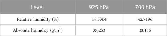
TABLE 2. Comparison of relative and absolute humidity at the 925 hPa and 700 hPa levels.

To further explore the causes, the sites with RH less than 30% in this space and time were located, and the precipitation intensity at different times of the corresponding stations was determined by using the surface automatic weather station data. Figure 8A shows that the data points that meet an RH of less than 30% are concentrated in the North China Plain region, and there are also a small number distributed in the Northeast Plain and the Yunnan-Guizhou Plateau regions. Figures 8B–G show that the first 3 hours to the previous hour have less precipitation and a smaller impact range, and the subsequent one to 3 hours of precipitation increase obviously and the scope of influence is expanded. This proves to some extent the accuracy of the results of the SHAP model; that is, when the RH is less than 30%, it makes a positive contribution to the prediction of precipitation, increasing the probability of predicting precipitation. In order to verify the spatiotemporal characteristics of water vapor transport (He et al., 2007), the 850-hPa level horizontal wind field and geopotential height reanalysis data from April, May and June 2016 were used, and the 850-hPa wind pressure field representing the low altitude level was obtained after averaging the time, respectively (Figures 9G–I). Using the multi-layer wind field and specific humidity reanalysis data under 1,000 hPa to 300 hPa in April, May and June, the integral of 1,000 hPa to 300 hPa in the vertical direction after taking the time average, respectively, obtained the water vapor flux field representing the whole layer (Figures 9D–F) and the water vapor flux field of the 850-hPa single layer (Figures 9A–C). It can be clearly seen that a very deep south-branch trough appears in the southwest direction of China (Figures 9G–I), which is consistent with the findings of (Ke et al., 2021), and the southwest wind blows before the trough (east side of the trough), which can be used as a warm conveyor belt. The air makes an upward movement to transport warm and humid air over the Indian Ocean and the Bay of Bengal to the middle and low latitudes of China. A powerful cold vortex system (Northeast Cold Vortex) appears in the northeast direction, and a distinct westerly wind conveyor belt appears on the south side of the cold vortex, bringing cooler air masses to North China. In addition, studies have shown that the Northeast Cold Vortex affects precipitation in eastern China and has a clear correlation with the Western Pacific Subtropical High (Liu et al., 2015; Gao, 2022). There is a pronounced subtropical high pressure in the southeast direction (Yuan et al., 2020) from April to June, and on the eve of the first north jump of the subtropical high pressure, a southeast monsoon will be on its southwestern side to deliver warm and humid air flow through the tropical western Pacific Ocean to southeast China. Warm and humid air currents from the southwest and sub-high edges intersect with strong cold air from the northeast around at 33°–40°N, roughly coinciding with the data point concentration area. The connection between the above weather systems transports water vapor, heat and momentum from low to higher latitudes, creating conditions for cloud rain to form in mid- and high-latitude regions. The water vapor flux field is basically the same as the wind field situation, and the low and middle latitudes have obvious southwest air flow and west wind air flow to transport a large amount of water vapor to the North China Plain. This feature is most pronounced in June.

FIGURE 8

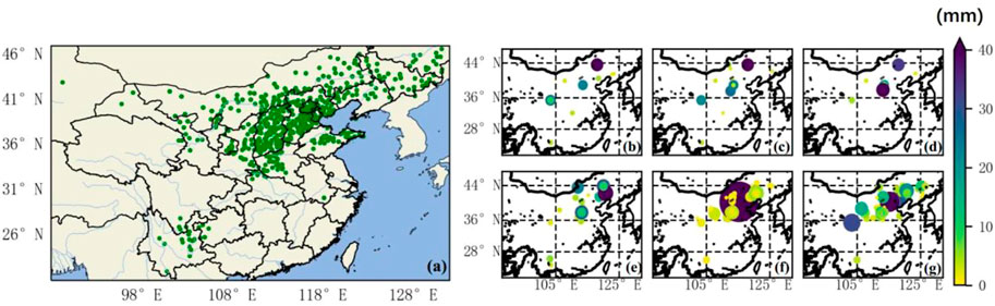
FIGURE 8. (A) Data point distribution plot with relative humidity of less than 30%. The hourly rainfall intensity distribution map for the data points in (A): (B) rainfall for the first 3 hours; (C) rainfall for the first 2 hours; (D) rainfall the previous hour; (E) rainfall in the next hour; (F) rainfall in the next 2 hours; (G) rainfall in the next 3 hours.

FIGURE 9

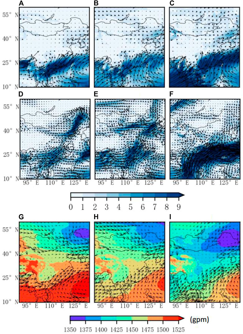
FIGURE 9. Monthly-averaged single-layer water vapor flux field at 850 hPa (unit: $\mathbf{g}$· ${\mathbf{P}\mathbf{a}}^{-\mathbf{1}}$· ${\mathbf{m}}^{-\mathbf{1}}$· ${\mathbf{s}}^{-\mathbf{1}}$):(A) April; (B) May; (C) June. Monthly-averaged whole-layer water vapor flux field of 1,000–300 hPa (unit: $\mathbf{g}$· ${\mathbf{P}\mathbf{a}}^{-\mathbf{1}}$· ${\mathbf{m}}^{-\mathbf{1}}$· ${\mathbf{s}}^{-\mathbf{1}}$): (D) April; (E) May; (F) June. Monthly average geopotential height (gpm) and wind vector field (m/s) at 850 hPa. The vector denotes the size and direction of wind and water vapor flux, the shading indicates the value of potential height: (G) April; (H) May; (I)June.

Further statistical analysis of the observation data with less than 30% RH reveals that the observation time distribution of the data has obvious diurnal variation characteristics (Figure 10G). Maximums occur at 0300–1,000 and 1,500–1800 Beijing time (BJT), respectively, of which the number of occurrences at 0300–1000 BJT accounts for more than 63% of the total number of times, and the average time of data point occurrence is about 0900 BJT. This is associated with low-level jet stream with obvious daily variations in intensity (Yan et al., 2021). The northern hemisphere’s low-level jet streams are strong in the morning and weakest in the afternoon, generally in the south or southwest, appearing on the west or north edge of the subtropical high pressure, and play a role in transporting heat, water vapor and momentum to the lower atmosphere. The updraft is mostly located on the left or at the front of the axis of jet stream, and another obvious feature is that on its north or west side there is a lot of cold air sinking from the middle and pelagic layers, which flows all the way to the front and converges with the airflow from the south or east, further strengthening the airflow in the ascendant branch. When the warm and humid air is transported north to the bottom of the drier and cooler air, a convectively unstable stratification is formed, and under the trigger of the upward movement on the left side of the low-level jet stream, it is easy for convective precipitation to be produced, such as heavy rain and hail, and even tornado weather. The same meteorological elements were selected and the data were analyzed. The day was divided into three time periods (0300–1000 BJT, 1,100–1800 BJT, and 1900–0200 BJT) and then the time averaged to obtain the 1,000–300 hPa whole layer of the water vapor flux field (Figures 10D–F) and the 850 hPa single-layer water vapor flux field (Figure 10A–C) in the three periods. Among them, after the average value of the water vapor flux value of the 850-hPa single-layer, the situation of each time period is as follows: the time period of 0300–1000 BJT has a maximum value; the time period of 1900–0200 BJT has a large value; and the time period of 1,100–1800 BJT has a minimum value. This is basically consistent with the diurnal variation characteristics of low-level jet streams. Therefore, the water vapor transport at 0300–1000 BJT is related to the low-level jet streams from the southwest direction.

FIGURE 10

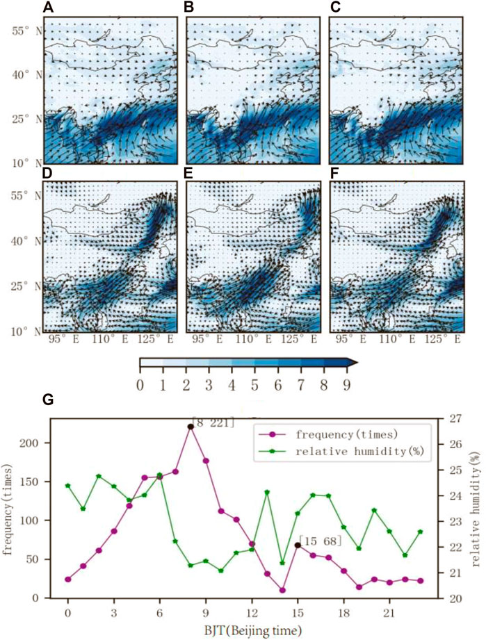
FIGURE 10. Diurnal variation of the single-layer water vapor flux field at 850 hPa (unit: $\mathbf{g}$· ${\mathbf{P}\mathbf{a}}^{-\mathbf{1}}$· ${\mathbf{m}}^{-\mathbf{1}}$· ${\mathbf{s}}^{-\mathbf{1}}$): (A) 0300–1000 BJT; (B) 1,100–1800 BJT; (C) 1900–0200 BJT. Diurnal variation of the water vapor flux field of the whole layer of 1,000–300 hPa (unit: $\mathbf{2}$· ${\mathbf{10}}^{\mathbf{2}}$· $\mathbf{g}$· ${\mathbf{m}}^{-\mathbf{1}}$· ${\mathbf{s}}^{-\mathbf{1}}$): (D) 0300–1000 BJT; (E) 1,100–1800 BJT; (F) 1900–0200 BJT. (G) The number of times the relative humidity is less than 30% during different data observations, and the corresponding relative humidity value. The vector represents the water vapor flux value.

In summary, through the humidity conditions, wind pressure fields, and water vapor flux fields of different atmospheric levels, we have preliminarily verified the conjecture that precipitation in areas with relative humidity of less than 30% comes from non-local water vapor transport. At the same time, the seemingly abnormal output of the SHAP model is thus physically explained, which verifies its rationality.

4.4 Advantage and limitation

Using SHAP to explain the machine learning model used to predict meteorological elements, its advantages and reliability have been tested in previous studies (Ghafarian et al., 2022; Song et al., 2022; Tang et al., 2022). For instance, Tang et al. (2022) combined machine learning and SHAP to find potential climate remote links and improve the prediction of other climate signals. Their results show that SHAP can eliminate the difference in the importance of features caused by the selection of different indicators, which is meaningful for revealing the objective phenomenon that has not been found, and it helps to fill the gap in the interpretability of machine learning models. Compared with other studies that use machine learning to predict precipitation (Min et al., 2019; Li et al., 2021a; Lao et al., 2021; Lao et al., 2021), nevertheless, our present work focuses on interpreting the output of the model, exploring the features and models, and the influence between different features. SHAP is an after-the-fact interpretation approach that is suitable for any machine learning model. In the future, we need to find a meteorology-based physical interpretation model for SHAP to apply to the actual operation of machine learning model interpretation. In addition, for the anomalies in relative humidity that appear in this paper, we will further explore the physical mechanisms of MCSs (Mishra, 2018).

5 Conclusion

Based on ERA5 reanalysis data, AHI observation and inversion data carried by the Himawari-8 meteorological satellite, and high-density automatic weather station data, a QPE model for MCSs was constructed by using a random forest algorithm, and the interpretation of the output of the random forest was explored by using a SHAP model. The main conclusions can be summarized as follows:

The output of the random forest model for QPE can be analyzed by the SHAP model for global and local feature influence, and the feature importance ranking and local contribution values can be obtained. The importance ranking obtained by SHAP model is completely consistent with the outputs of random forest importance function. This SHAP method can display the importance ranking of global features with positive/negative contribution values (e.g., current precipitation, column water vapor/black body temperature, cloud base height), and can visualize the marginal contribution values of local features under interaction. Taking current precipitation, tbb and cloud base height as examples, the local influence was analyzed and combined with objective facts, which proved the reliability of the SHAP model applied to the random forest model for QPE. Clusters of features and samples can be achieved through SHAP, assisting in the search for highly relevant features as well as high-quality samples. Taking tbb as another example, the SHAP model can visualize the interaction between features, which is conducive to exploring the influence of features on the output of the model and the interaction between features, and even the physical meaning implied in the interaction. In contrast, by analyzing anomalies in the RH Shapley value, we can still find a relatively reasonable physical explanation to justify its results. In general, our findings show that combining the RF and SHAP methods provides a valuable way to interpret the output of machine learning models for satellite-based QPE, as well as an important basis for the selection of input variables for satellite-based QPE.

Data availability statement

The original contributions presented in the study are included in the article/supplementary material, further inquiries can be directed to the corresponding author.

Author contributions

ZH: Methodology, formal analysis, results, and discussion, and writing—original draft preparation. RF, SZ, WZ, YB, JL, and BW: Discussion and writing reviewing and editing. YY: Conceptualization, methodology, results, and discussion, and writing—reviewing and editing. All authors contributed to the article and approved the submitted version.

Funding

This study was supported by National Natural Science Foundation of China (42222503 and 42175098). The data that support the findings of this study are available based the request.

Acknowledgments

We acknowledge the High Performance Computing Center of Nanjing University of Information Science & Technology for their support of this work.

Conflict of interest

BW was employed by Boyan Information Technology (Xi’an) Co Ltd.

The remaining authors declare that the research was conducted in the absence of any commercial or financial relationships that could be construed as a potential conflict of interest.

Publisher’s note

All claims expressed in this article are solely those of the authors and do not necessarily represent those of their affiliated organizations, or those of the publisher, the editors and the reviewers. Any product that may be evaluated in this article, or claim that may be made by its manufacturer, is not guaranteed or endorsed by the publisher.

References

Adler, R. F., and Mack, R. A. (1984). Thunderstorm cloud height–rainfall rate relations for use with satellite rainfall estimation techniques. J. Appl. Meteorology Climatol. 23 (2), 280–296. doi:10.1175/1520-0450(1984)023<0280:tchrrf>2.0.co;2

CrossRef Full Text | Google Scholar

Atkinson, P. M., and Tatnall, A. (1997). Introduction Neural networks in remote sensing. Int. J. Remote Sens. 18, 699–709. doi:10.1080/014311697218700

CrossRef Full Text | Google Scholar

Ban, N., Schmidli, J., and Schär, C. (2015). Heavy precipitation in a changing climate: Does short-term summer precipitation increase faster? Geophys. Res. Lett. 42, 1165–1172. doi:10.1002/2014GL062588

CrossRef Full Text | Google Scholar

Barredo Arrieta, A., Díaz-Rodríguez, N., Del Ser, J., Bennetot, A., Tabik, S., Barbado, A., et al. (2019). Explainable Artificial Intelligence (XAI): Concepts, taxonomies, opportunities and challenges toward responsible AI. Inf. Fusion 58, 82–115. doi:10.1016/j.inffus.2019.12.012

CrossRef Full Text | Google Scholar

Bi, Y., Xiang, D., Ge, Z., Li, F., Jia, C., and Song, J. (2020). An interpretable prediction model for identifying N7-methylguanosine sites based on XGBoost and SHAP. Mol. Ther. - Nucleic Acids 22, 362–372. doi:10.1016/j.omtn.2020.08.022

PubMed Abstract | CrossRef Full Text | Google Scholar

Bochenek, B., and Ustrnul, Z. (2022). Machine learning in weather prediction and climate analyses—applications and perspectives. Atmosphere 13, 180. doi:10.3390/atmos13020180

CrossRef Full Text | Google Scholar

Breiman, L. (2001). Random forests. Mach. Learn. 45 (1), 5–32. doi:10.1023/A:1010933404324

CrossRef Full Text | Google Scholar

Brenner, I. S. (2004). The relationship between meteorological parameters and daily summer rainfall amount and coverage in west-central Florida. Am. Meteorological Soc. 19 (2), 286–300. doi:10.1175/1520-0434(2004)019<0286:TRBMPA>2.0.CO;2

CrossRef Full Text | Google Scholar

Chen, D., Guo, J., Yao, D., Feng, Z., and Lin, Y. (2020). Elucidating the life cycle of warm-season mesoscale convective systems in eastern China from the himawari-8 geostationary satellite. Remote Sens. 12, 2307. doi:10.3390/rs12142307

CrossRef Full Text | Google Scholar

Chen, P., Yihong, D., Yu, H., and Chunmei, H. U. (2007). Application of equivalent black body temperature in the forecast of tropical cyclone intensity. J. Geophys. Res. 21. 7471. doi:10.1029/2006JD007471

CrossRef Full Text | Google Scholar

Colman, B. R. (1990). Thunderstorms above frontal surfaces in environments without positive CAPE. Part II: Organization and instability mechanisms. Mon. Weather Rev. 118 (5), 1123–1144. doi:10.1175/1520-0493(1990)118<1123:tafsie>2.0.co;2

CrossRef Full Text | Google Scholar

El-Alfy, E. S., and Mohammed, S. (2020). A review of machine learning for big data analytics: Bibliometric approach. Technol. Analysis Strategic Manag. 32, 984–1005. doi:10.1080/09537325.2020.1732912

CrossRef Full Text | Google Scholar

Feng, D. C., Wang, W. J., Mangalathu, S., and Taciroglu, E. (2021). Interpretable XGBoost-SHAP machine learning model for shear strength prediction of squat RC walls. J. Struct. Eng. 147, 04021173. doi:10.1061/(ASCE)ST.1943-541X.0003115

CrossRef Full Text | Google Scholar

Futrell, J., Gephart, R., Kabat-Lensch, E., McKnight, D., Pyrtle, A., Schimel, J., et al. (2005). Water: Challenges at the intersection of human and natural systems. Technical Report. doi:10.2172/1046481

CrossRef Full Text | Google Scholar

Gao, Z., Zhang, J., Yu, M., Liu, Z., Yin, R., Zhou, S., et al. (2022). Role of water vapor modulation from multiple pathways in the occurrence of a record-breaking heavy rainfall event in China in 2021. Earth Space Sci. 9, 2357. doi:10.1029/2022EA002357

CrossRef Full Text | Google Scholar

Gaur, Y., Jain, A., and Sarmonikas, G. (2020). Precipitation nowcasting using deep learning techniques. Report. doi:10.13140/RG.2.2.29845.86248

CrossRef Full Text | Google Scholar

Genuer, R., Poggi, J. M., and Tuleau-Malot, C. (2010). Variable selection using random forests. Pattern Recognit. Lett. 31 (14), 2225–2236. doi:10.1016/J.PATREC.2010.03.014

CrossRef Full Text | Google Scholar

Ghafarian, F., Wieland, R., Lüttschwager, D., and Nendel, C. (2022). Application of extreme gradient boosting and Shapley Additive explanations to predict temperature regimes inside forests from standard open-field meteorological data. Environ. Model. Softw. 156, 105466. doi:10.1016/j.envsoft.2022.105466

CrossRef Full Text | Google Scholar

Gray, S. (2011). Mesoscale meteorology in midlatitudes by Paul markowski and yvette richardson. Hoboken, NJ: Wiley.

Google Scholar

He, J., Sun, C., Liu, Y., Matsumoto, J., and Li, W. (2007). Seasonal transition features of large-scale moisture transport in the Asian-Australian monsoon region. Adv. Atmos. Sci. 24, 1–14. doi:10.1007/s00376-007-0001-5

CrossRef Full Text | Google Scholar

Hobbs, P. V. (1989). Research on clouds and precipitation: Past, present, and future, part I. Bull. Amer. Meteor. 70 (3), 282–285. doi:10.1175/1520-0477-70.3.282

CrossRef Full Text | Google Scholar

Johnsen, P. V., Riemer-Sørensen, S., DeWan, A. T., Cahill, M. E., and Langaas, M. (2021). A new method for exploring gene-gene and gene-environment interactions in GWAS with tree ensemble methods and SHAP values. BMC Bioinforma. 22 (1), 230. doi:10.1186/s12859-021-04041-7

CrossRef Full Text | Google Scholar

Ke, L., Shunwu, Z., Xia, S., Siyuan, C., and Qianqian, S. (2021). A synthetic study of the position difference of the southern branch trough of the qinghai-Ti-bet plateau based on objective identification. J J. Geoscience Environ. Prot. 09 (03), 182–194. doi:10.4236/gep.2021.93011

CrossRef Full Text | Google Scholar

Kim, Y., and Kim, Y. (2022). Explainable heat-related mortality with random forest and SHapley Additive exPlanations (SHAP) models. Sustain. Cities Soc. 79, 103677. doi:10.1016/j.scs.2022.103677

CrossRef Full Text | Google Scholar

Kuhnlein, M., Appelhans, T., Thies, B., and Nauss, T. (2014). Improving the accuracy of rainfall rates from optical satellite sensors with machine learning - a random forests-based approach applied to MSG SEVIRI. REMOTE Sens. Environ. 141, 129–143. doi:10.1016/j.rse.2013.10.026

CrossRef Full Text | Google Scholar

Kühnlein, M., Appelhans, T., Thies, B., and Nauss, T. (2014). Precipitation estimates from MSG SEVIRI daytime, nighttime, and twilight data with random forests. J. Appl. Meteorology Climatol. 53, 2457–2480. doi:10.1175/JAMC-D-14-0082.1

CrossRef Full Text | Google Scholar

Lao, P., Liu, Q., Ding, Y., Wang, Y., Li, Y., and Li, M. (2021). Rainrate estimation from FY-4A cloud top temperature for mesoscale convective systems by using machine learning algorithm. Remote. Sens. 13, 3273. doi:10.3390/rs13163273

CrossRef Full Text | Google Scholar

Li, X., Wu, C., Meadows, M. E., Zhang, Z., Lin, X., Zhang, Z., et al. (2021a). Factors underlying spatiotemporal variations in atmospheric PM2.5 concentrations in Zhejiang Province, China. Remote Sens. 13 (15), 3011. doi:10.3390/rs13153011

CrossRef Full Text | Google Scholar

Li, X., Yang, Y., Mi, J., Bi, X., Zhao, Y., Huang, Z., et al. (2021b). Leveraging machine learning for quantitative precipitation estimation from Fengyun-4 geostationary observations and ground meteorological measurements. Atmos. Meas. Tech. 14, 7007–7023. doi:10.5194/amt-14-7007-2021

CrossRef Full Text | Google Scholar

Lin, G., Chen, X., Fuab, Z., Zhao, Q., Fu, D., Guo, S., et al. (2007). Temporal-spatial diversities of long-range correlation for relative humidity over ChinaComparison of spatial interpolation methods for the estimation of precipitation patterns at different time scales to improve the accuracy of discharge simulations. Phys. A-STATISTICAL Mech. ITS Appl. Res. 38351 (2), 583146–583601. doi:10.1016/j.physa.2007.04.059Liu10.2166/nh.2020.146

CrossRef Full Text | Google Scholar

Liu, G., Feng, G., Qin, Y., Cao, L., Yao, H., and Liu, Z. (2015). Activity of cold vortex in Northeastern China and its connection with the characteristics of precipitation and circulation during 1960–2012. J. Geogr. Sci. 25, 1423–1438. doi:10.1007/s11442-015-1243-2

CrossRef Full Text | Google Scholar

Lundberg, S., Erion, G., and Lee, S. I. (2018). Consistent individualized feature attribution for tree ensembles. arXiv. doi:10.48550/arXiv.1802.03888

CrossRef Full Text | Google Scholar

Lundberg, S. M., Erion, G., Chen, H., DeGrave, A., Prutkin, J. M., Nair, B., et al. (2020). From local explanations to global understanding with explainable AI for trees. Nat. Mach. Intell. 2 (1), 56–67. doi:10.1038/s42256-019-0138-9

PubMed Abstract | CrossRef Full Text | Google Scholar

Mahlstein, I., and Knutti, R. (2010). Regional climate change patterns identified by cluster analysis. Clim. Dyn. 35, 587–600. doi:10.1007/s00382-009-0654-0

CrossRef Full Text | Google Scholar

Mangalathu, S., Hwang, S. H., and Jeon, J. S. (2020). Failure mode and effects analysis of RC members based on machine-learning-based SHapley Additive exPlanations (SHAP) approach. Eng. Struct. 219, 110927. doi:10.1016/j.engstruct.2020.110927

CrossRef Full Text | Google Scholar

Min, H., Haolan, Z., Bingjian, W., Gang, L., and Li, Z. (2022). Interpretable predictive model for shield attitude control performance based on XGboost and SHAP. Sci. Rep. 12 (1), 18226. doi:10.1038/s41598-022-22948-w

PubMed Abstract | CrossRef Full Text | Google Scholar

Min, M., Bai, C., Guo, J., Sun, F., Liu, C., Wang, F., et al. (2019). Estimating summertime precipitation from himawari-8 and global forecast system based on machine learning. IEEE Trans. Geoscience Remote Sens. 57, 2557–2570. doi:10.1109/TGRS.2018.2874950

CrossRef Full Text | Google Scholar

Mishra, A. K. (2018). Remote sensing of convective clouds using multi-spectral observations and examining their variability over India. Remote Sens. Appl. Soc. Environ. 12, 23–29. doi:10.1016/j.rsase.2018.08.002

CrossRef Full Text | Google Scholar

Molinie, G., and Jacobson, A. R. (2004). Cloud-to-ground lightning and cloud top brightness temperature over the contiguous United States. J. Geophys. Res. Atmos. 109 (D13), 3593. doi:10.1029/2003JD003593

CrossRef Full Text | Google Scholar

Nesbitt, S., Cifelli, R., and Rutledge, S. (2006). Storm morphology and rainfall characteristics of TRMM precipitation features. Mon. Weather Rev. - Mon. WEATHER Rev. 134, 2702–2721. doi:10.1175/MWR3200.1

CrossRef Full Text | Google Scholar

Ning, Y., Ong, M. E. H., Chakraborty, B., Goldstein, B. A., Ting, D. S. W., Vaughan, R., et al. (2022). Shapley variable importance cloud for interpretable machine learning. Patterns 3 (4), 100452. doi:10.1016/j.patter.2022.100452

PubMed Abstract | CrossRef Full Text | Google Scholar

Parker, M., Rutledge, S. A., and Johnson, R. H. (2000). Cloud-to-ground lightning in linear mesoscale convective systems. Mon. Weather Rev. 129 (5), 1232–1242. doi:10.1175/1520-0493(2001)1292.0.CO;2

CrossRef Full Text | Google Scholar

Pathy, A., Meher, S., and Balasubramaniyan, B. P. (2020). Predicting algal biochar yield using eXtreme Gradient Boosting (XGB) algorithm of machine learning methods. Algal Res. 50, 102006. doi:10.1016/j.algal.2020.102006

CrossRef Full Text | Google Scholar

Pérez-Castrillo, D., and Sun, C. (2022). The proportional ordinal Shapley solution for pure exchange economies. Games Econ. Behav. 135, 96–109. doi:10.1016/j.geb.2022.06.001

CrossRef Full Text | Google Scholar

Rasmussen, K. L., Chaplin, M. M., Zuluaga, M. D., and Houze, R. A. (2016). Contribution of extreme convective storms to rainfall in South America. J. Hydrometeorol. 17, 353–367. doi:10.1175/JHM-D-15-0067.1

CrossRef Full Text | Google Scholar

Ren, J., Xu, G., Zhang, W., Leng, L., Xiao, Y., Wan, R., et al. (2021). Evaluation and improvement of FY-4A AGRI quantitative precipitation estimation for summer precipitation over complex topography of western China. Remote Sens. 13 (21), 4366. doi:10.3390/rs13214366

CrossRef Full Text | Google Scholar

Roth, A. E., and Shapley, L. S. (1991). The Shapley value: Essays in honor of lloyd S. Shapley. Economica 101, 123. doi:10.2307/2554979

CrossRef Full Text | Google Scholar

Rui, X., and Wunsch, D. (2005). Survey of clustering algorithms. IEEE Trans. Neural Netw. 16 (3), 645–678. doi:10.1109/TNN.2005.845141

PubMed Abstract | CrossRef Full Text | Google Scholar

Ruoyun, M., Jianhua, S., and Xinlin, Y. (2021). An eight-year climatology of the warm-season severe thunderstorm environments over North China. J Atmos. Res. 254, 105519. doi:10.1016/j.atmosres.2021.105519

CrossRef Full Text | Google Scholar

Sanò, P., Panegrossi, G., Casella, D., Di Paola, F., Milani, L., Mugnai, A., et al. (2015). The passive microwave neural network precipitation retrieval (PNPR) algorithm for AMSU/MHS observations: Description and application to European case studies. Atmos. Meas. Tech. 8, 837–857. doi:10.5194/amt-8-837-2015

CrossRef Full Text | Google Scholar

Shapley, L. S. (1952). A value for n-person games. Santa Monica, CA: RAND Corporation.

Google Scholar

Song, X., Hao, Y., and Jim Yeh, T. C. (2022). Spatial-temporal behavior of precipitation driven karst spring discharge in a mountain terrain. J. Hydrology 612, 128116. doi:10.1016/j.jhydrol.2022.128116

CrossRef Full Text | Google Scholar

Tang, G., Ma, Y., Long, D., Zhong, L., and Hong, Y. (2015). Evaluation of GPM Day-1 IMERG and TMPA Version-7 legacy products over Mainland China at multiple spatiotemporal scales. J. Hydrology 533, 152–167. doi:10.1016/j.jhydrol.2015.12.008

CrossRef Full Text | Google Scholar

Tang, Y., Duan, A., Xiao, C., and Xin, Y. (2022). The prediction of the Tibetan plateau thermal condition with machine learning and Shapley additive explanation. Remote Sens. 14, 4169. doi:10.3390/rs14174169

CrossRef Full Text | Google Scholar

Todd, A., Collins, M., Lambert, F. H., and Chadwick, R. (2018). Diagnosing ENSO and global warming tropical precipitation shifts using surface relative humidity and temperature. J. Clim. 31 (4), 1413–1433. doi:10.1175/JCLI-D-17-0354.1

CrossRef Full Text | Google Scholar

Vilone, G., and Longo, L. (2020). Explainable artificial intelligence: A systematic review. arXiv. doi:10.48550/arXiv.2006.00093

CrossRef Full Text | Google Scholar

Wang, K., Tian, J., Zheng, C., Yang, H., Ren, J., Liu, Y., et al. (2021). Interpretable prediction of 3-year all-cause mortality in patients with heart failure caused by coronary heart disease based on machine learning and SHAP. Comput. Biol. Med. 137, 104813. doi:10.1016/j.compbiomed.2021.104813

PubMed Abstract | CrossRef Full Text | Google Scholar

Wen, X., Xie, Y., Wu, L., and Jiang, L. (2021). Quantifying and comparing the effects of key risk factors on various types of roadway segment crashes with LightGBM and SHAP. Accid. Analysis Prev. 159, 106261. doi:10.1016/j.aap.2021.106261

CrossRef Full Text | Google Scholar

Wieland, R., Lakes, T., and Nendel, C. (2020). Using SHAP to interpret XGBoost predictions of grassland degradation in Xilingol. Geo Sci. Model. Dev. 13, 9–16. doi:10.5194/gmd-2020-59

CrossRef Full Text | Google Scholar

Xu, K., Zhong, L., Ma, Y., Zou, M., and Huang, Z. (2020). A study on the water vapor transport trend and water vapor source of the Tibetan Plateau. Theor. Appl. Climatol. 140 (3-4), 1031–1042. doi:10.1007/s00704-020-03142-2

CrossRef Full Text | Google Scholar

Yan, Y., Xuhui, C., Xuesong, W., Yucong, M., and Yu, S. (2021). Low-level jet climatology of China derived from long-term radiosonde observations. J. Geophys. Res. Atmos. 126 (20). doi:10.1029/2021JD035323

CrossRef Full Text | Google Scholar

Yang, K., Tang, Q., and Hui, L. (2022). Precipitation recycling ratio and water vapor sources on the Tibetan Plateau. Sci. China Earth Sci. 65, 584–588. doi:10.1007/s11430-021-9871-5

CrossRef Full Text | Google Scholar

Yang, Y., Wang, H., Chen, F., Zheng, X., Fu, Y., and Zhou, S. (2018). TRMM-based optical and microphysical features of precipitating clouds in summer over the yangtze–huaihe river valley, China. Pure Appl. Geophys. 176, 357–370. doi:10.1007/s00024-018-1940-8

CrossRef Full Text | Google Scholar

Yogiraj, S., and Ashish, M. (2016). A survey on unsupervised clustering algorithm based on K-means clustering. J Int. J. Comput. Appl. 156 (8), 156–159. doi:10.5120/ijca2016912481

CrossRef Full Text | Google Scholar

Yuan, Y., Gao, H., and Ding, T. (2020). The extremely north position of the Western Pacific subtropical high in summer of 2018: Important role of the convective activities in the Western Pacific. J Int. J. Climatol. 40 (3), 1361–1374. doi:10.1002/joc.6274

CrossRef Full Text | Google Scholar

Zheng, X., Yang, Y., Yuan, Y., Cao, Y. n., and Gao, J. (2021). Comparison of macro- and microphysical properties in precipitating and non-precipitating clouds over central-eastern China during warm season. Remote Sens. 14, 152. doi:10.3390/rs14010152

CrossRef Full Text | Google Scholar

Ziegler, A., and Koenig, I. R. (2014). Mining data with random forests: Current options for real-world applications. Wiley Interdiscip. Reviews-Data Min. Knowl. Discov. 4 (1), 55–63. doi:10.1002/widm.1114

CrossRef Full Text | Google Scholar