Prediction model and consequence analysis for riverine oil spills

Long-distance oil and gas pipelines play an important role in ensuring energy imports, but can cause riverine oil spills and threaten public health and the environment. The emergency disposal of spilled oil is affected by a number of factors such as the difficulty of disposal and the long recovery cycle; however, there are deficiencies in the understanding of river oil spills. In this study, a prediction model of the river oil spill trajectory based on the random walk particle tracking algorithm was constructed. The performance of the model was tested by simulating the Enbridge Line 6B Oil Discharge scenario occurred in the United States in 2010. The temporal and spatial variations of the oil pollution zone in downstream and vertical directions were studied, and the interception effects on the arrival time of oil in key sections were obtained. Results showed that after the spilled oil entered the surface water body, the tiny oil droplets generated by crushing can remain underwater for a long time, making them difficult to detect and intercept. It can further combine with suspended particles in the water, settle, and pollute the riverbed, which has a greater potential for harm and risk. The model offers helpful information for the first-phase emergency response for riverine oil spills.

1 Introduction

Long oil and gas pipelines play an essential role in ensuring the security of imported energy. To meet the rising energy demand driven by rapid economic growth, China is experiencing a third wave of pipeline construction, with the lengths of crude oil and petroleum product pipelines ranking fourth and third, respectively, in the world (Li et al., 2021). Meanwhile, there is growing concern regarding the effects of oil spills (Zheng and Huang, 2017). Countries such as the United States, Canada, and China have created emergency management systems to guide responses to oil spills (Li et al., 2016).

According to National Transportation Safety Board’s (NTSB) reports (National Transportation Safety Board (NTSB)), a total of 486 pipeline incidents occurred in America between 2010 and 2019, of which 151 involved oil spills, accounting for 31% of the total pipeline incidents. Forty-four of these oil spills reached inland water systems and caused environmental pollution, accounting for 9% of the total pipeline incidents. These incidents spilled more than four million gallons of oil, including diesel, gasoline, and crude oil, damaging fresh water resources, the soil environment, and ecosystems to varying degrees, and causing over 270 million dollars in economic losses. One of the most famous incident is the Enbridge Line 6B Oil Spill incident. The pipeline ruptured at approximately 6 p.m. on 25 July 2010. The crude oil (DilBit) spilled from the ruptured segment, seeped into the ground and the nearby wetland, and flowed to the Talmadge Creek. The emergency response was initiated 17 h after the spill. The discharged DilBit volume was estimated to be approximately 3,192 m³ (843,444 gallons) and drifted downstream along the Talmadge Creek before entering the Kalamazoo River. The impacted area, including the river, floodplains, and wetlands along the banks, exceeded 20 km². River channel restoration lasted until October 2014.

There are more than 175,000 km of onshore oil and gas pipelines in China. Many pipelines cross large rivers within their territory, such as the Yangtze River, the Yellow River, and transboundary rivers, such as the Lancang River. An oil spill from such pipelines could cause serious environmental pollution and even have an international impact (Chang et al., 2014; Beyer et al., 2016). Modeling the fate and transport of discharged oil in inland rivers is critical for risk assessment and oil response (Amir-Heidari et al., 2019) and these efforts date back to the 1970s (Tsahalis, 1979). River morphology (meanders, branches, artificial constructions etc.) and ambient environment variation (rain, wind et al.) significantly influence river flow through multiple aspects (Yapa et al., 1994; Rakesh and B, 2018). The spilled oil may transform into a film, droplet, emulsion, aggregate, or other forms within 24 h of the spill (Afenyo et al., 2016; Brussaard et al., 2016), which brings potential challenges to the modeling field. Compared with the development of tools for oil spills in the ocean (Keramea et al., 2021; Zhao et al., 2021), studies on oil transportation in inland waterways are limited (Goeury et al., 2014; Kvočka et al., 2021), and new attempts at model optimization and calibration are still made by researchers around the world (Jiang et al., 2021; Li et al., 2022).

The longitudinal distribution of oily pollutants is one of the primary concerns in response to an oil spill in a river. Timely calculation will help in the decision-making of appropriate first-phase action to control the expansion of polluted areas and prevent even worse consequences. River hydrodynamics provide basic flow data for particle tracking algorithms. With the long-term development of numerical approaches for the dynamic model, a large number of mature software packages are available, and many researchers have discussed the computational performance of these models in different scenarios and scales (Jowett and Duncan, 2012; Bürgler et al., 2022). The contaminated area, which is significantly influenced by the longitudinal flow velocity, is hundreds of kilometers in length. It is verified that a one-dimensional hydraulic model can provide accurate results with less effort and computational requirements for large-scale modeling tasks if well calibrated (Horritt and Bates, 2002; de Paiva et al., 2013).

In this study, a random walk particle tracking algorithm using one-dimensional unsteady hydrodynamics was constructed. Data of real-time flow fluctuation and variation of atmospheric parameters can be exchanged at high speeds using the random walk model. The performance of the model was tested by simulating the Enbridge Line 6B Oil Discharge scenario. The consequences with and without containment measures were compared to provide insights into the effectiveness and challenges of emergency operations.

2 Methodology

2.1 Hydrodynamic model

The HEC-RAS software (Hydraulic Engineering Center, developed by the United States Army Corps of Engineers), which yields reliable results in the hydrodynamic modeling of natural rivers, was used for one-dimensional unsteady hydrodynamic simulations in this study. The software uses a weighted four-point implicit finite difference method (Gary, 2020) to solve the Saint-Venant equations by discretization and iteration:

$\frac{\partial A}{\partial t}+\frac{\partial S}{\partial t}+\frac{\partial Q}{\partial x}-q_l=0(1)$

$\frac{\partial Q}{\partial t}+\frac{\partial \left(vQ\right)}{\partial x}+gA\left(\frac{\partial z}{\partial x}+S_f\right)=0(2)$

where t is time, x is the longitudinal distance along the river channel, A is the cross-sectional area of the portion of the channel occupied by the flow, Q is river discharge, S is the cross-sectional area of the portion of the channel without water flow, q_l is lateral incoming flow, v is flow velocity, g is the gravitational acceleration, and S_f is friction slope.

The current study focused on the river segment impacted by the Enbridge Line 6 B Oil Discharge, which stretches from Talmadge Creek near Marshall to downstream Morrow Lake. River bathymetry was created by interpolating the field data from the United States Geological Survey (USGS) report (Reneau et al., 2015) with the bathymetry interpolation tool from Merwade et al. (2008). The bathymetry map was then merged with a digital elevation model (DEM, with a resolution of 1 m × 1 m) published by the USGS in order to produce a corrected elevation map of the study area. The constructed main channel model for the HEC-RAS was 64.27 km in length, with an average slope of 0.72‰. The model contained a total of 3893 cross sections with spacing of 1.4–30.9 m apart. Inflow was applied to nine cross sections, the locations of which are illustrated in Figure 1.

FIGURE 1

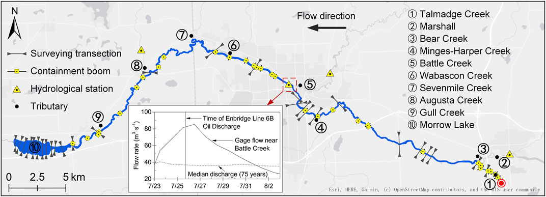
FIGURE 1. Study area.

Flow data from the 12th of April to the 16th of April 2013 were used to verify the model (Reneau et al., 2015). The model was calibrated using water surface elevation and discharge data from USGS stations 04105500, SR1485, and SR0585 by adjusting Manning’s roughness coefficients. More details can be found in the supplementary data.

2.2 Particle-tracking model

In the Lagrangian scheme, the displacement components of each particle in the longitudinal (x), lateral (y), and vertical (z) directions in Cartesian coordinates at time (t + Δt) (i.e., $x_i^{t+\Delta t}$, $y_i^{t+\Delta t}$, and $z_i^{t+\Delta t}$) were determined by its location at time t, advective movement, and diffusive transport during the time interval Δt (Wu et al., 2019). The Visser scheme was employed to describe the vertical movement of particles (Visser, 1997). The governing equations are as follows.

$x_i^{t+\Delta t}=x_i^t+u_i^t\Delta t+R_{-1}^1\sqrt{2{\sigma }_R^{-1}{D}_x^t\Delta t}(3)$

$y_i^{t+\Delta t}=y_i^t+v_i^t\Delta t+R_{-1}^1\sqrt{2{\sigma }_R^{-1}{D}_y^t\Delta t}(4)$

$z_i^{t+\Delta t}=z_i^t+w_i^t\Delta t+{D_z^t}^{\prime }\Delta t+R_{-1}^1\sqrt{2{\sigma }_R^{-1}{D}_{z1}^t\Delta t}(5)$

Here i is the number index of a particle, Δt is the time step; $u_i^t$ and $v_i^t$ are streamwise and lateral flow velocity components at location ($x_i^t$, $y_i^t$) (m·s⁻¹), respectively; $w_i^t$ is the average vertical velocity of the particle between t and t + Δt, which is calculated using the Stokes equation (m·s⁻¹); $R_{-1}^1$ is a uniform distribution between −1 and 1; ${\sigma }_R$ is the standard deviation of random number R, which is set at 1/3 (Visser, 1997) and $D_x^t$, $D_y^t$, and $D_z^t$ denote the streamwise, lateral, and vertical turbulent diffusivity coefficients at time t, respectively.

In the present study, the transverse flow velocity ($v_i^t$) was ignored because the longitudinal drifting of the oil particles was more valuable for a fast emergency response. The longitudinal velocity ($u_i^t$) is assumed to obey the law of the wall (Jones and Garcia, 2018), which is written as:

$\frac{u_i^t}{u_{*}}=\frac{1}{\kappa }\ln \left(\frac{u_{*}{z}_i^t}{\nu }\right)+5.5(6)$

where $u_{*}$ denotes the shear velocity of the flow (m·s⁻¹); ν denotes the dynamic viscosity of water (m²·s⁻¹); and κ denotes the von Karman constant (0.41).

The streamwise and lateral diffusions, $D_x^t$ and $D_y^t$, are given by (Garcia, 2008):

$D_x^t=D_y^t=0.6H{u}_{*}(7)$

For $D_z^t$, the parabolic-constant profile (Rijn, 1984) was employed and expressed as:

$D_z^t=\{\begin{array}{ll}0.25\kappa u_{*}H& \frac{z}{H}\ge 0.5\\ z_1\left(1-\frac{z_1}{H}\right)\kappa u_{*}& \frac{z}{H}<0.5\end{array}(8)$

where H is the water depth (m). In the lower half of the depth, $D_z^t$ is estimated for location z₁, which is given by $z_1=z_i^t+{D_z^t}^{\prime }\Delta t/2$.

A reflective boundary condition was used when the oil particles exceeded the left, right, and bottom boundaries of the channel. When the particles surfaced, they were assumed to be absorbed into the oil slick. The resuspension probability, p, was calculated to determine whether the particles would reenter the water column (Nordam et al., 2019). p is given by

$p=1-e^{-∆t\cdot \lambda }(9)$

where λ is the lifetime of the oil at the surface (Nordam et al., 2019).

In particular, a random depth is assigned if the particle is resuspended; otherwise, the mass loss of the oil droplet due to evaporation should be calculated during the surfaced duration.

2.3 Spill scenarios

Based on a series of documents released by the National Transportation Safety Board, in the present model, the leakage entered the upstream of Talmadge Creek at the cross section located approximately 2.5 km away from the confluence of Talmadge Creek and the Kalamazoo River, and the start time was 18:00 on 25 July 2010. Oil particles were released at a rate of 720 per hour in the calculation domain for 10 h. Based on the oil droplet size distribution, which was reported in the literature based on the breakup of oil in water (Li et al., 2009; Johansen et al., 2015; Zeinstra-Helfrich et al., 2016), nine oil droplet sizes, that is, diameters of 0.5 mm, 2 mm, 4 mm, 6 mm, 8 mm, 10 mm, 12 mm, 16 mm, and 20 mm, were considered. The density of oil at different temperatures is given by (Berry et al., 2012):

${\rho }_{oil}={\rho }_{ref}\left[1.0-8.0\times {10}^{-4}\left(T-T_{ref}\right)\right](10)$

The density of oil after evaporation was expressed by (Berry et al., 2012),

${\rho }_{oil}={\rho }_{ref}\left(1.0+0.018F_{ev}\right)(11)$

where ρ_oil is the density of the spilled oil (kg·m⁻³); ρ_ref is the reference density at a reference temperature T_ref, which is approximately 920 kg m⁻³ at 20°C; T is the temperature (°C), equal to 23°C; F_ev is the mass loss in percentage terms (%); and t is the duration of evaporation (min).

Based on the measured data obtained by Waterman (Waterman, 2015), a fitting function in logarithmic form (R² = 0.985) that describes the mass loss due to evaporation was introduced as follows:

$F_{ev}=1.961\ln \left(t\right)(12)$

The hydraulic data were calculated using the HEC-RAS software using the flow data between July 25th and 31st, 2010 (Reneau et al., 2015). The particle-tracing algorithm was performed using MATLAB software. The computational time step is 2 s.

Two scenarios, one with containment booms and the other with no measures, were conducted. The containment booms were positioned similarly to those in actual situations and extended 0.05 m deep underwater. Figure 2.

FIGURE 2

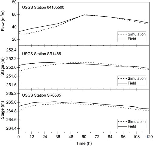
FIGURE 2. Comparison between simulation and survey results.

3 Results

3.1 Drift and distribution in scenario with no containment measure

When no containment measure was taken, particles with different sizes exhibited similar drifting trajectories in the simulated domain. Figure 3 illustrates the maps of the particle positions when the particle diameter equals 1 mm. The black arrows in the figure indicate the leading edges of the particle swarm at 1 h, 6 h, 12 h, 24 h, 72 h, and 120 h. The particles arrived at Battle Creek at approximately 19.5 h, which roughly matched the time when a resident reported the appearance of an oil slick near Battle Creek, according to documents released by the National Transportation Safety Board.

FIGURE 3

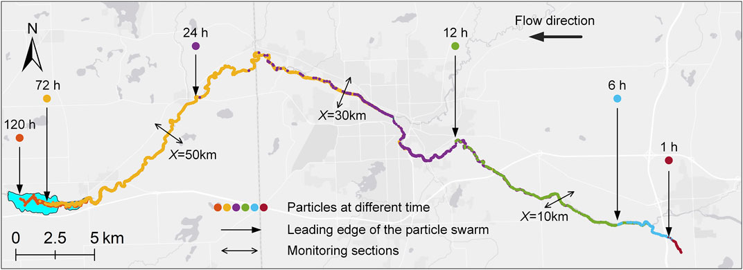
FIGURE 3. Particle position vs. time (particle diameter 0.5 mm).

Figure 4 shows the statistics for the 10th, 25th, 50th, 75th, and 90th percentiles of the distance drifted downstream of the particle swarm, as well as the temporal variation in the average distance. Overall, the polluted zone continued to expand. The 90th and 10th percentiles represent the positions of the front and rear edges of the polluted zone, respectively. The length of the polluted zone in the downstream direction can then be calculated as the difference between the 90th and 10th percentiles. This was calculated as 12.06 km, 22.81 km, 29.61 km, and 34.96 km, at 12 h, 24 h, 36 h, and 48 h, respectively, after the oil entered the water. The length of the polluted zone decreased after 48 h, because the front edge arrived at the downstream boundary of the simulated area.

FIGURE 4

FIGURE 4. Statistics on distance drifted downstream by particles (particle diameter 0.5 mm).

Plotting the means of the particle swarm’s longitudinal position (X) and vertical position (Z) at different times provides insight into how the center of the particle swarm varies spatially and temporally. As shown in Figure 5, the dimensionless height Z/H was used as well as Z/H = 1.0, which represents the water surface. In general, as the particle size increased from 0.5 mm to 10 mm, the vertical velocity, which is influenced by the buoyancy force, increased. Advective movement driven by buoyancy dominated the vertical position of the particles; thus, more particles (larger than 4 mm) appeared close to the water surface. Small particles were gradually dispersed in water and forced by diffusive movement. After a trip of 10 km downstream, the center of the 0.5 mm particle cloud stabilized at approximately Z/H = 0.6.

FIGURE 5

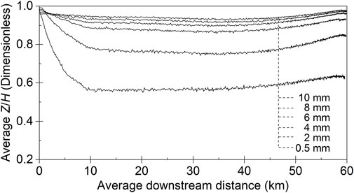
FIGURE 5. Variation in the center of mass of particle swarm (Z/H = 1.0 represents the water surface).

3.2 Impact of containment measure

After the containment booms were added in the same positions as the actual containment booms that were installed in real response operations, particles with different diameters changed their movement paths. The monitoring sections were set in the model at downstream distances of 10 km, 30 km, and 50 km, as shown in Figure 3. As shown in Figure 6A, the number of particles passing through each section was determined. The containment booms implanted before the monitoring section at a distance of 10 km exhibited a slight interception effect on particles smaller than 10 mm. Approximately 26.12% of the 16 mm particles and 65.93% of the 20 mm particles were contained in the upstream booms. At a distance of 30 km, the containment rates for the 8 mm, 10 mm, and 20 mm particles increased to 7.57%, 19.72%, and 91.23%, respectively. At a distance of 50 km, the corresponding containment rates further increased to 27.54%, 52.55%, and 95.11%, respectively. Unlike large oil droplets, which migrated in the upper part of the water column, small oil droplets were hardly blocked by the implanted booms as these particles were suspended over depth, as revealed in the previous section. The containment effectiveness was enhanced by increasing the number of containment booms. However, their relationship is complex because it is also affected by the actual particle properties and hydraulic conditions.

FIGURE 6

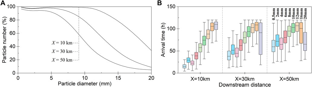
FIGURE 6. Statistics on oil particles at cross-sections located at downstream distance X = 10 km, 20 km, and 30 km respectively: (A) Percentage of particles passing through each section; (B) Arrival time of particles with different sizes.

Statistical analysis was performed for the time when the particles arrived at each monitoring cross section. In the model with no containment measure implanted, the mean time for particles to reach the sections 10 km, 30 km, and 50 km downstream was 11.80 ± 0.41, 35.15 ± 1.34, and 55.01 ± 1.84 h, respectively. The average arrival times in the presence of containment booms are plotted in Figure 6B. We found that the diffusion of oil droplets greater than 6 mm was slowed by the containment booms.

4 Discussion

This study simulated the drifting trajectory of oil droplets in the Kalamazoo River with and without containment measures. Although the sizes of the droplets are artificial to some extent, they provide insight into the difficulty of the cleanup after the spill. Containment measures have an apparent effect on floating slicks. However, as the statistics revealed, small droplets (less than 6 mm in diameter in our simulation) that stayed below the water surface for a long period were hardly stopped by the containment booms. In contrast to their low proportion of leakage volume, these particles, in all probability, potentially pose tremendous hazards, as they would further break into micro-sized particles and coagulate with the suspended solid particles in the water column to form dense aggregates, known as oil–particle aggregates (OPAs). The formed OPAs tend to reach lower waters, deposit on the riverbed, and are resuspended when the water is agitated. With regards to the Enbridge Line 6 B Oil Spill, it took more than 4 years, with costs of up to 1.21 billion dollars, to clean the residual oil from the 56.5-km-long river segment where OPAs were detected. The deposition of OPAs on the downstream riverbed varied with the properties of the oil, sand, and natural environment. Interested readers may refer to our previous study for more information on the formation and transport of OPAs (Wang et al., 2020b; Li et al., 2022).

To obtain a rapid view of the oil fate along the river for a timely emergency response after a spill, a one-dimensional hydrodynamic model by HEC-RAS was employed to provide the depth-averaged streamwise velocities, which were considered as the major factor contributing to the longitudinal transport of particles. The setting enabled fast exchange of data between the real-time flow fluctuations and subsequent particle tracing programs for large-scale river basins. However, it cannot precisely describe the lateral distribution of oil, especially when one is interested in the fate of oil in a lake, reservoir, oxbow, etc. Under these circumstances, two-dimensional or coupled 1D/2D hydrodynamics are required as opposed to a one-dimensional model. In addition, the range of oiled riverbanks cannot be detailed. Using two- or three-dimensional hydrodynamics with a sufficiently fine meshed domain may be used to identify the location where the particle landed on the bank. Predicting the amount of retained oil along the bank is relatively difficult, as our previous study showed that it is related to multiple factors such as the roughness of the substrate, slope of the bank, hydraulic scouring force, and plant types along the bank (Wang et al., 2020a). Further studies are underway to understand the quantitative relationship between oil retention and the related factors.

The absorption and re-entrainment of oil droplets at the water surface remains unclear. In the present study, a probability function is introduced to describe the resuspension probability of a particle. Although the simplification is not sensitive to the big picture of particle distribution in such a large-scale river basin, further refinement, calibration, and validation of the approach are necessary in the future.

5 Conclusion

Oil spills in inland rivers have serious consequences and cause considerable losses. Modeling the fate and transport of discharged oil in inland rivers, especially the longitudinal distribution, is critical for risk assessment and oil response. In the present work, a random walk particle tracking algorithm was constructed to provide a quick view of oil transport along the river for a timely emergency response after a spill. The main conclusions are as follows.

(1) The model uses one-dimensional hydrodynamics to drive particles. A velocity profile was employed in the vertical direction to correct the streamwise velocity at different positions. A Visser scheme was employed to describe the vertical movement of particles. A probability function was applied to describe the re-entrainment of particles at the water surface.

(2) When no containment measure was taken, particles with different sizes exhibited similar drifting trajectories in the longitudinal direction. Vertical statics revealed that large particles appeared close to the water surface due to advective movement driven by buoyancy, while small particles dispersed in water gradually due to diffusive movement.

(3) Containment measures had an apparent effect on floating slicks. However, small droplets (less than 6 mm in diameter in our simulation) that stayed below the water surface for longer period of time were hardly stopped by containment booms. Although small droplets comprise a low proportion of the leakage volume, these particles potentially pose tremendous hazards.

(4) The model is a tool for calculating the temporal and spatial variations of the impacted zone and the arrival time at key cross-sections after the oil spill and offers helpful information for the first-phase emergency response. Further refinement and calibration of the simplifications employed in the model will be necessary in the future.

Data availability statement

The original contributions presented in the study are included in the article/Supplementary Material, further inquiries can be directed to the corresponding author.

Author contributions

All authors listed have made a substantial, direct, and intellectual contribution to the work and approved it for publication.

Funding

This work was supported by Fundamental Research Funds for the Central Universities (No. FRF-TP-20-003A3), and the National Key R&D Program of China (No. 2016YFC0802104).

Conflict of interest

The authors declare that the research was conducted in the absence of any commercial or financial relationships that could be construed as a potential conflict of interest.

Publisher’s note

All claims expressed in this article are solely those of the authors and do not necessarily represent those of their affiliated organizations, or those of the publisher, the editors and the reviewers. Any product that may be evaluated in this article, or claim that may be made by its manufacturer, is not guaranteed or endorsed by the publisher.

Supplementary material

The Supplementary Material for this article can be found online at: https://www.frontiersin.org/articles/10.3389/fenvs.2022.1054839/full#supplementary-material

References

Afenyo, M., Veitch, B., and Khan, F. (2016). A state-of-the-art review of fate and transport of oil spills in open and ice-covered water. Ocean. Eng. 119, 233–248. doi:10.1016/J.OCEANENG.2015.10.014

CrossRef Full Text | Google Scholar

Amir-Heidari, P., Arneborg, L., Lindgren, J. F., Lindhe, A., Rosén, L., Raie, M., et al. (2019). A state-of-the-art model for spatial and stochastic oil spill risk assessment: A case study of oil spill from a shipwreck. Environ. Int. 126, 309–320. doi:10.1016/J.ENVINT.2019.02.037

PubMed Abstract | CrossRef Full Text | Google Scholar

Berry, A., Dabrowski, T., and Lyons, K. (2012). The oil spill model OILTRANS and its application to the Celtic Sea. Mar. Pollut. Bull. 64, 2489–2501. doi:10.1016/j.marpolbul.2012.07.036

PubMed Abstract | CrossRef Full Text | Google Scholar

Beyer, J., Trannum, H. C., Bakke, T., Hodson, P. v., and Collier, T. K. (2016). Environmental effects of the deepwater Horizon oil spill: A review. Mar. Pollut. Bull. 110, 28–51. doi:10.1016/J.MARPOLBUL.2016.06.027

PubMed Abstract | CrossRef Full Text | Google Scholar

Brussaard, C. P. D., Peperzak, L., Beggah, S., Wick, L. Y., Wuerz, B., Weber, J., et al. (2016). Immediate ecotoxicological effects of short-lived oil spills on marine biota. Nat. Commun. 7 (1 7), 11206–11211. doi:10.1038/ncomms11206

PubMed Abstract | CrossRef Full Text | Google Scholar

Bürgler, M., Vetsch, D. F., Boes, R. M., and Vanzo, D. (2022). Systematic comparison of 1D and 2D hydrodynamic models for the assessment of hydropeaking alterations. River Res. Appl. 1–18. doi:10.1002/rra.4051

CrossRef Full Text | Google Scholar

Chang, S. E., Stone, J., Demes, K., and Piscitelli, M. (2014). Consequences of oil spills: A review and framework for informing planning. Ecol. Soc. 19, art26. Published online: May 09, 2014. doi:10.5751/ES-06406-190226

CrossRef Full Text | Google Scholar

de Paiva, R. C. D., Buarque, D. C., Collischonn, W., Bonnet, M.-P., Frappart, F., Calmant, S., et al. (2013). Large-scale hydrologic and hydrodynamic modeling of the Amazon River basin. Water Resour. Res. 49, 1226–1243. doi:10.1002/wrcr.20067

CrossRef Full Text | Google Scholar

Garcia, M. (2008). Sedimentation Engineering. Reston, VA, USA: American Society of Civil Engineers. doi:10.1061/9780784408148

CrossRef Full Text | Google Scholar

Gary, W. B. (2020). HEC-RAS river analysis system hydraulic reference manual. Davis, CA, USA: US ARMY CORPS OF ENGINEERS HYDROLOGIC ENGINEERING CENTER HEC. Available at: https://www.hec.usace.army.mil/confluence/rasdocs/ras1dtechref/latest (Accessed October 28, 2022).

Google Scholar

Goeury, C., Hervouet, J. M., Baudin-Bizien, I., and Thouvenel, F. (2014). A Lagrangian/Eulerian oil spill model for continental waters. J. Hydraulic Res. 52, 36–48. doi:10.1080/00221686.2013.841778

CrossRef Full Text | Google Scholar

Horritt, M. S., and Bates, P. D. (2002). Evaluation of 1D and 2D numerical models for predicting river flood inundation. J. Hydrol. X. 268, 87–99. doi:10.1016/S0022-1694(02)00121-X

CrossRef Full Text | Google Scholar

Jiang, P., Tong, S., Wang, Y., and Xu, G. (2021). Modelling the oil spill transport in inland waterways based on experimental study. Environ. Pollut. 284, 117473. doi:10.1016/J.ENVPOL.2021.117473

PubMed Abstract | CrossRef Full Text | Google Scholar

Johansen, Ø., Reed, M., and Bodsberg, N. R. (2015). Natural dispersion revisited. Mar. Pollut. Bull. 93, 20–26. doi:10.1016/J.MARPOLBUL.2015.02.026

PubMed Abstract | CrossRef Full Text | Google Scholar

Jones, L., and Garcia, M. H. (2018). Development of a rapid response riverine oil–particle aggregate formation, transport, and fate model. J. Environ. Eng. New. York. 144, 04018125. doi:10.1061/(ASCE)EE.1943-7870.0001470

CrossRef Full Text | Google Scholar

Jowett, I. G., and Duncan, M. J. (2012). Effectiveness of 1D and 2D hydraulic models for instream habitat analysis in a braided river. Ecol. Eng. 48, 92–100. doi:10.1016/J.ECOLENG.2011.06.036

CrossRef Full Text | Google Scholar

Keramea, P., Spanoudaki, K., Zodiatis, G., Gikas, G., and Sylaios, G. (2021). Oil spill modeling: A critical review on current Trends, Perspectives, and challenges. J. Mar. Sci. Eng. 9, 181. doi:10.3390/jmse9020181

CrossRef Full Text | Google Scholar

Kvočka, D., Žagar, D., and Banovec, P. (2021). A review of river oil spill modeling. Water 13, 1620. Page 1620 13. doi:10.3390/W13121620

CrossRef Full Text | Google Scholar

Li, P., Cai, Q., Lin, W., Chen, B., and Zhang, B. (2016). Offshore oil spill response practices and emerging challenges. Mar. Pollut. Bull. 110, 6–27. doi:10.1016/J.MARPOLBUL.2016.06.020

PubMed Abstract | CrossRef Full Text | Google Scholar

Li, Q., Zhao, M., Zhang, B., Wen, W., Wang, L., Zhang, X., et al. (2021). Current construction status and development trend of global oil and gas pipelines in 2020 (in Chinese). Oil Gas Storage Transp. 40, 1330–1337. doi:10.6047/j.issn.1000-8241.2021.12.002

CrossRef Full Text | Google Scholar

Li, Y., Zhu, Z., Soong, D. T., Khorasani, H., Wang, S., Fitzpatrick, F., et al. (2022). FluOil: A Novel tool for modeling the transport of oil-particle aggregates in inland waterways. Front. Water 3, 180. doi:10.3389/frwa.2021.771764

CrossRef Full Text | Google Scholar

Li, Z., Lee, K., King, T., Boufadel, M. C., and Venosa, A. D. (2009). Evaluating Chemical dispersant Efficacy in an experimental wave Tank: 2—Significant factors determining in Situ oil droplet size distribution. Environ. Eng. Sci. 26, 1407–1418. https://home.liebertpub.com/ees 26. doi:10.1089/EES.2008.0408

CrossRef Full Text | Google Scholar

Merwade, V., Cook, A., and Coonrod, J. (2008). GIS techniques for creating river terrain models for hydrodynamic modeling and flood inundation mapping. Environ. Model. Softw. 23, 1300–1311. doi:10.1016/J.ENVSOFT.2008.03.005

CrossRef Full Text | Google Scholar

National Transportation Safety Board (NTSB) (2022). Accident Investigation report. Available at: https://www.ntsb.gov/investigations/AccidentReports/Pages/Reports.aspx?mode=Pipeline (Accessed October 30, 2022).

Google Scholar

Nordam, T., Kristiansen, R., Nepstad, R., and Röhrs, J. (2019). Numerical analysis of boundary conditions in a Lagrangian particle model for vertical mixing, transport and surfacing of buoyant particles in the water column. Ocean. Model. (Oxf). 136, 107–119. doi:10.1016/j.ocemod.2019.03.003

CrossRef Full Text | Google Scholar

Rakesh, B., and B, S. W. (2018). Data and calibration challenges for spill response models. J. Environ. Eng. New. York. 144, 04017109. doi:10.1061/(ASCE)EE.1943-7870.0001319

CrossRef Full Text | Google Scholar

Reneau, P. C., Soong, D. T., Hoard, C. J., and Fitzpatrick, F. A. (2015). Hydrodynamic assessment data associated with the July 2010 line 6B spill into the Kalamazoo River, Michigan, 2012–14. Report 2015-1205. U.S. Geological Survey Open-File Juneau, AL, USA. doi:10.3133/ofr20151205

CrossRef Full Text

Rijn, L. C. van (1984). Sediment transport, Part II: Suspended load transport. J. Hydraul. Eng. 110, 1613–1641. doi:10.1061/(asce)0733-9429(1984)110:11(1613)

CrossRef Full Text | Google Scholar

Tsahalis, D. T. (1979). Contingency planning for oil spills: RIVERSPILL - a river simulation model. Int. Oil Spill Conf. Proc. 1979, 27–36. doi:10.7901/2169-3358-1979-1-27

CrossRef Full Text | Google Scholar

Visser, A. (1997). Using random walk models to simulate the vertical distribution of particles in a turbulent water column. Mar. Ecol. Prog. Ser. 158, 275–281. doi:10.3354/meps158275

CrossRef Full Text | Google Scholar

Wang, S., Xu, S., Yang, Y., Jin, L., Wang, Y., and Zhang, J. (2020a). Retention behavior of spilled oil along river bank. J. China Univ. Petroleum Ed. Nat. Sci. 44, 144–150.

Google Scholar

Wang, S., Yang, Y., Zhu, Z., Jin, L., and Ou, S. (2020b). Riverine deposition pattern of oil–particle aggregates considering the coagulation effect. Sci. Total Environ. 739, 140371. doi:10.1016/j.scitotenv.2020.140371

PubMed Abstract | CrossRef Full Text | Google Scholar

Waterman, D. M. (2015). Laboratory Tests of oil-particle Interactions in a Freshwater riverine environment with Cold lake Blend Weathered Bitumen. Urbana, IL, USA: University of Illinois.

Google Scholar

Wu, X., Liang, D., and Zhang, G. (2019). Estimating the accuracy of the random walk simulation of mass transport processes. Water Res. 162, 339–346. doi:10.1016/J.WATRES.2019.06.027

PubMed Abstract | CrossRef Full Text | Google Scholar

Yapa, P. D., Shen, H. T., and Angammana, K. S. (1994). Modeling oil spills in a river—Lake system. J. Mar. Syst. 4, 453–471. doi:10.1016/0924-7963(94)90021-3

CrossRef Full Text | Google Scholar

Zeinstra-Helfrich, M., Koops, W., and Murk, A. J. (2016). How oil properties and layer thickness determine the entrainment of spilled surface oil. Mar. Pollut. Bull. 110, 184–193. doi:10.1016/J.MARPOLBUL.2016.06.063

PubMed Abstract | CrossRef Full Text | Google Scholar

Zhao, L., Nedwed, T., and Mitchell, D. (2021). Review of the Science behind oil spill fate models: Are Updates Needed? Int. Oil Spill Conf. Proc. 2021, 687874. doi:10.7901/2169-3358-2021.1.687874

CrossRef Full Text | Google Scholar

Zheng, H., and Huang, W. (2017). Development status and prospect of safety insurance technologies for oil&gas pipelines and storage and transportation facilities (in Chinese). Oil Gas Storage Transp. 36, 1–7. doi:10.6047/j.issn.1000-8241.2017.01.001

CrossRef Full Text | Google Scholar