
94% of researchers rate our articles as excellent or good
Learn more about the work of our research integrity team to safeguard the quality of each article we publish.
Find out more
ORIGINAL RESEARCH article
Front. Environ. Sci., 20 January 2023
Sec. Atmosphere and Climate
Volume 10 - 2022 | https://doi.org/10.3389/fenvs.2022.1054235
This article is part of the Research TopicHydro-Climate Extremes and Natural Disasters During Global Warming: Observation, Projection, and MitigationView all 11 articles
 Kexin Zhu1,2,3,4
 Qiqi Yang2,3,4
 Shuliang Zhang2,3,4*Shuai Jiang1,2,3,4
 Tianle Wang2,3,4
 Jinchen Liu2,3,4
 Yuxuan Ye2,3,4
High-resolution radar rainfall data have great potential for rainfall predictions up to 6 h ahead (nowcasting); however, conventional extrapolation approaches based on in-built physical assumptions yield poor performance at longer lead times (3–6 h), which limits their operational utility. Moreover, atmospheric factors in radar estimate errors are often ignored. This study proposed a radar rainfall nowcasting method that attempts to achieve accurate nowcasting of 6 h using long short-term memory (LSTM) networks. Atmospheric conditions were considered to reduce radar estimate errors. To build radar nowcasting models based on LSTM networks (LSTM-RN), approximately 11 years of radar, gauge rainfall, and atmospheric data from the UK were obtained. Compared with the models built on optical flow (OF-RN) and random forest (RF-RN), LSTM-RN had the lowest root-mean-square errors (RMSE), highest correlation coefficients (COR), and mean bias errors closest to 0. Furthermore, LSTM-RN showed a growing advantage at longer lead times, with the RMSE decreasing by 17.99% and 7.17% compared with that of OF-RN and RF-RN, respectively. The results also revealed a strong relationship between LSTM-RN performance and weather conditions. This study provides an effective solution for nowcasting radar rainfall at long lead times, which enhances the forecast value and supports practical utility.
Nowcasting is defined as local detailed forecasting at lead times of 1–6 h using any method, along with a full description of the current weather (Wang et al., 2017). It is a key instrument for predicting rapidly changing and severe weather (Sun et al., 2022), such as heavy rain and violent thunderstorms (Pulkkinen et al., 2019). It is also critical for small, mountainous, and urban watersheds, where stream flow responds rapidly to rainfall (Imhoff et al., 2020). Generally, nowcasting offers benefits to many sectors of the real world, such as emergency services, energy management, and flood early warning systems (Wilson et al., 2010).
Numerical weather prediction (NWP) and radar-based rainfall prediction (radar nowcasting) are the two main approaches to nowcasting with different application scales (Pulkkinen et al., 2019). By feeding current weather conditions into atmospheric models, NWP models try to simulate atmospheric behavior and provide rainfall predictions on a global and mesoscale (Cuo et al., 2011). However, the predictions offered by NWP systems for short lead times (0–2 h) are often unsatisfactory because of their coarse temporal resolution and low update frequency (Imhoff et al., 2020), along with the difficulties in model spin-up and data assimilation (Sun, 2005; Pierce et al., 2012; Sun et al., 2014; Buehner and Jacques, 2020). Consequently, alternative methods based on radar that provide more timely and accurate predictions have been widely used. With high spatial and temporal resolutions, typically 1 km and 5 min, respectively, radar rainfall products are regarded as having great potential for short-term rainfall forecasts (Ravuri et al., 2021). Radar nowcasting is the process of extrapolating rainfall based on apparent motion that has been analyzed using the most recent radar images (Wang al., 2017). Currently, radar extrapolation methods can be classified as object- or pixel-based (Zahraei et al., 2013). The object-based methods, as represented by Storm Cell Identification and Tracking (SCIT) and Thunderstorm Identification, Tracking, Analysis and Nowcasting (TITAN) proposed by the US, consider storm events as separate objects thus performing well in detecting and tracking specific thunderstorm cells (Dixon and Wiener, 1993; Vila et al., 2008). The pixel-based methods, on the contrary, outperform in forecasting convective storms and precipitation in stratocumulus clouds by using full motion fields (Grecu and Krajewski, 2000; Berenguer et al., 2011). One recent progress is the optical flow-based method. It introduces computer vision techniques to make extrapolation of radar maps, and displays high flexibility and accuracy (Bowler et al., 2004).
However, owing to the separated tracking and extrapolation steps, as well as the in-built non-linear physical assumptions, the conventional extrapolation approaches have limited success. They struggle to capture complex rainfalls, and show a decreasing skill at longer lead times (Golding, 1998; Liguori and Rico-Ramirez, 2013; Ravuri et al., 2021). In this context, machine learning methods, especially artificial neural networks (NNs), have been introduced in nowcasting. Based on self-adaptive principles that learn from samples and grasp functional relationships between data, NN has been widely used to predict, recognize, and classify a wide range of weather events, and is also one of the most appealing strategies for nowcasting (Valverde Ramírez et al., 2005; Hernández et al., 2016). Koizumi (Koizumi, 1999) found that models built on NN have higher skill scores than other nowcasting models, when using weather data of 1 year for training. Apart from the improved prediction accuracy, the NN trained by Foresti et al. (2019) using 10-year weather radar data in the Swiss Alps effectively learned and reproduced growth and decay patterns in the atmosphere, which is intrinsically challenging to predict. With the development of computer science, deep learning has risen drastically and expanded swiftly in many data-rich scientific disciplines, including nowcasting (Ayzel et al., 2020). Composed of multiple processing layers, the improved networks support the exploration of insight and complex structures of datasets. They overcome the drawbacks of traditional NNs, such as ineffective training practices and inability to manage extensive data, thus, becoming popular in handling complicated issues (Jia et al., 2017; Van et al., 2020). For example, Agrawal et al. (2019) presented a nowcasting model based on convolutional NN that, compared with other commonly used methods, performed favorably. For time-series problems, Chen et al. (2021) used long short-term memory (LSTM) networks to build a nowcasting model, and the results exhibited an evidently reduced prediction error. A wide variety of fantastic networks have been proposed and have made significant progress in nowcasting (Shi et al., 2015; Shi et al., 2017; Tian et al., 2019; Kumar et al., 2020; Luo et al., 2020), but a critical problem is that lead times in past studies have been relatively short (usually 0–2 h) (Schmidhuber, 2015; Kang et al., 2020). In fact, deep learning, particularly LSTM networks with fantastic memory ability (Gers et al., 2002), have great promise for achieving longer lead times in nowcasting.
In addition, previous research has focused on upgrading nowcasting algorithms while disregarding the many errors in radar rainfall estimates, which could result in numerous uncertainties. These uncertainties in radar data are carried over into radar nowcasting and grow with increasing rainfall rates (Ebert et al., 2004; Liguori et al., 2012). It is well known that the accuracy of radar rainfall estimates is affected by various factors, such as spurious echoes (e.g., from the ground, sea, and aero-planes), attenuation of the radar signal (Krämer et al., 2005; Villarini and Krajewski, 2009), and beam blockage (Joss and Lee, 1995). Actually, apart from the radar measurement instruments, weather conditions can also lead to radar estimation errors, which have rarely been explored in previous studies (Seo et al., 1999; Song et al., 2017). Recently, researchers have begun to focus on this issue. Dai and Han (Dai and Han, 2014) were the first to incorporate the wind field into the construction of a radar rainfall uncertainty model, and the proposed model improved the correlation coefficients of most rainfall events by over 10%. Yang et al. (2020) considered multiple atmospheric fields to build a radar rainfall uncertainty adjustment model, and the results indicated a satisfactory performance of the model under high relative humidity and wind speed.
Therefore, this study incorporated atmospheric data into radar rainfall nowcasting with the aim of reducing radar estimate errors and improving prediction accuracy. A framework for nowcasting radar rainfall with long lead times of 1–6 h using LSTM networks was established. To investigate the performance of the proposed models at different altitudes and weather conditions, models were built using approximately 11 years of radar, gauge rainfall, and atmospheric data across the UK. Two other methods, optical flow (OF) and random forest (RF), were also built to further demonstrate the strengths of the proposed models.
The UK is located on Europe’s western shore, between 49°N and 61°N. Influenced by the west wind and the Atlantic Ocean, the UK has a cloudy and rainy climate, with an average of 1,000 mm rainfall every year. Rainfall in the UK is affected by geographic location to some extent; generally, the further west and the higher the altitude, the greater the rainfall. Extreme rainfall events are predicted to become more common as global temperatures rise, and the increased intensity of rainfall affects the frequency and severity of surface water floods, particularly in urban areas.
The radar rainfall data used in this study, with a spatial resolution of 1 km and temporal resolution of 5 min, were downloaded from the website (https://catalogue.ceda.ac.uk/) supplied by the UK Met Office. Sufficient data were collected from 2007 to 2017. The data were subjected to extensive processing by the NIMROD system for corrections with regards to several sources of radar errors (Song et al., 2017). The NIMROD radar rainfall data are one of the best available sources of rainfall information (Zhu et al., 2014). The 5-min radar rainfall data were adjusted at a 1-h rate to make it compatible with the hourly gauge data. Then, the radar rainfall value of the corresponding gauge was extracted for modelling at each station.
Gauge rainfall data with resolutions of .2 mm and 1 h from 40 tilting bucket rain gauges between 2007 and 2017 (except for very few sites) were collected from the Met Office Integrated Data Archive System Land and Marine Surface Stations dataset. Atmospheric data, including air pressure, relative humidity, temperature, wind direction, and wind speed, were obtained from the same source (Met Office, 2019). The Met Office built the Meteorological Monitoring System at each station to collect data at a resolution of 1 min. The data were then aggregated into hourly data. The Met Office was responsible for ensuring the quality of the data (Met Office, 2012). Forty gauging stations were used for modeling, as shown in Figure 1 (the labeled stations KOI and EGDM were used as demonstration examples in Section 4.1). The lowest and highest altitudes of these stations were 4.27 m, and 246.21 m, respectively. These stations were separated into three classes depending on altitude for subsequent analysis (Sections 4.2–4.4).
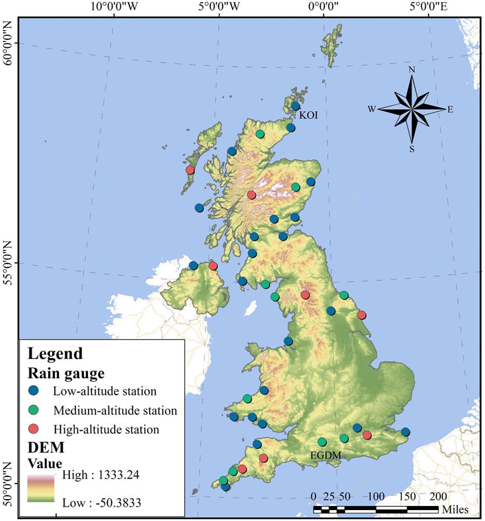
FIGURE 1. Locations of 40 stations in the UK study area with terrain elevation.
The basic architecture of a NN includes the input, output, and hidden layers. Recurrent NNs (RNNs) are a variant of traditional NNs that introduce a cyclic structure. Owing to this structure, the outputs of a given input can be influenced not only by the current input but also by the residual state left over from prior calculations (Warner and Misra, 1996). RNNs are, thus, well-suited in simulating time series and other dynamical processes that are clearly reliant on history (Le et al., 2017). LSTM, an improved type of RNN, replaces the neurons in a regular RNN with an upgraded memory unit; each LSTM memory unit includes an input gate, output gate, a forget gate, and memory cells. Compared with RNN, LSTM can solve complicated, artificial long-time-lag challenges that earlier RNNs could not (Hochreiter and Schmidhuber, 1997).
The LSTM architecture used in this study consisted of three layers: an input layer (radar rainfall and atmospheric data at each time step), a hidden layer, and an output layer (gauge rainfall at a certain lead time). Figure 2 shows the LSTM architecture used for modeling at 1-h lead time. The models were constructed based on this architecture according to the following steps:
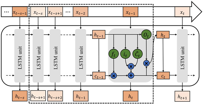
FIGURE 2. Architecture of the LSTM networks used in this study:
Step 1: Build the initial model (the selection of hyper-parameters can be found in Section 4.1).
Step 2: Normalize the data. Perform MinMaxScaler normalization on the datasets x (input) and h (output). The MinMaxScaler normalization formula is as follows:
Where
Step 3: Divide the data. Take normalized datasets x and h before 2016 as training data and the rest as test data.
Step 4: Organize the data and train the model. The training data and test data were organized as the architecture illustrated in Figure 2. The radar rainfall series and corresponding atmospheric data were used as input nodes, with the gauge rainfall serving as the target variable. To improve the generalization ability of the model and avoid overfitting, the organized data were randomly shuffled. The rainfall predicted by this model was denormalized before it was used as the final result.
The LSTM-RN models of the 40 stations with 1-h lead time were generated using the prior process. Similar procedures were performed to build the LSTM-RN models with lead times of 2–6 h.
Random forest (Breiman, 2001) is a conceptually simple machine-learning algorithm that combines the bagging ensemble learning theory with the random subspace method. It is made up of numerous decision tree classification modules and is highly efficient with large datasets. The tree-based machine learning method displayed high prediction accuracy (Speiser et al., 2019); therefore, it was adopted in this study to build comparative models.
The RF-RN models used in this study were constructed as follows:
Step 1: Randomly select N separate sample datasets from the training datasets as the training subset of each decision tree (the selection of N is discussed in Section 4.1).
Step 2: Establish a categorical regression tree for each sample dataset to generate N decision trees. For each node of the decision tree, the variable subset was randomly sampled from the original dataset, and the optimal variable was selected from the subset using the Gini index minimum criterion for node splitting and branching.
Step 3: Each categorical regression tree grew recursively from top to bottom, and stopped growing when the minimum size of the leaf nodes was reached. Subsequently, all the decision trees were combined into a random forest.
Step 4: The radar rainfall data and atmospheric data from the test sets were fed into the constructed model, and N decision trees were used to predict. The regression value was the average of the predicted outcomes of each decision tree.
In the field of computer vision, OF is typically considered as a collection of techniques to infer velocity patterns or fields from a series of image frames (Liu et al., 2015; Woo and Wong, 2017). For rainfall prediction, Ayzel et al. (2019) developed a set of tracking models based on two OF formulations, Sparse (Lucas and Kanade, 1981) and Dense (Kroeger et al., 2016), as well as two extrapolation techniques. The OF models built were an open benchmark for radar nowcasting. In this study, we used the dense model, which utilized a dense inverse search (DIS) algorithm to construct a continuous displacement field from two consecutive radar images. The DIS, a global OF algorithm proposed by Kroeger et al. (2016), can explicitly estimate the velocity of each image pixel based on the analysis of two continuous radar images.
This study used the “rainymotion” codebase, provided by Ayzel et al., to build the second type of comparative models, which is available at the following link: https://github.com/hydrogo/rainymotion.
Figure 3 shows the experimental flowchart. The data division and model construction processes have been described above, and the following paragraphs describe the three analysis parts.
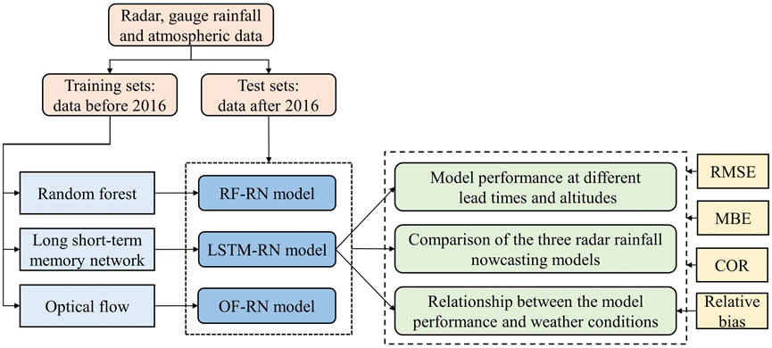
FIGURE 3. Schematic diagram of the experimental design.
First, the accuracy of the LSTM-RN models at different lead times and altitudes was investigated to better understand the performance pattern and further explore the causes of the difference in accuracy. The lead times ranged from 1 h to 6 h, as described in Section 3.1. Owing to the large number of gauges, it was impossible to obtain the exact performance of each model; however, roughly averaging the error indicator results of all models would miss the underlying causes of the models’ varied performance. Thus, we divided the stations into three classes based on their altitude (Figure 2) and compared the performance of the models at different altitude classes. Models with altitudes <75 m, >75 m and <150 m, and >150 m and <250 m were classified as low, medium, and high altitudes, respectively. Similar studies have also divided the gauge stations into three altitude classes (Milewski et al., 2015). The thresholds in this study were determined based on the characteristics of the data. With such thresholds, the number of data points in each class was approximately the same, and the differences between classes were enlarged as much as possible. The corresponding results are presented in Section 4.2.
Second, we constructed two types of comparative models, the RF-RN and OF-RN models, and ran identical rainfall nowcasting experiments. Four rainfall events were chosen to visually evaluate the prediction abilities of the models, and error indices were calculated to quantitatively assess the performance of the models from 1 to 6 h lead times. The corresponding results are presented in Section 4.3.
Finally, to investigate the relationship between the LSTM-RN model performance and diverse weather conditions, the test sets were divided into five classes depending on the rainfall rate (R) and relative humidity (H): classes A1–A5: R = (0, .2] (.2, .4] (.4, .8] (.8, 1.6], and R > 1.6 mm/h by rainfall rate; classes B1–B5: H = [0,80) [80,85) [85,90) [90,95), and H > 95% by relative humidity. The corresponding results are presented in Section 4.4.
Three error indices, namely, root-mean-square error (RMSE), mean bias error (MBE), and correlation coefficient (COR), were selected to evaluate the models. The RMSE, MBE, and COR were defined as follows:
where
The RMSE is the square root of the average of squared errors and is often used to measure the differences between the predicted or simulated values and the true values. This metric was chosen to quantify the accuracy of the prediction results, and a lower RMSE suggested a better match to the true value. The MBE assesses the average overestimation or underestimation of accumulated rainfall, with a perfect score of 0. This index was selected to investigate the deviation direction and extent of the model’s prediction, that is, the model’s tendency to underestimate or overestimate rainfall. The COR provides correlation information between the predicted or simulated values and the true values, which can indicate the model’s ability to capture the subsequent rain-fall trends in this study. COR ranges from –1 to 1, with a higher COR indicating better recognition.
Moreover, to eliminate the effect of magnitude, we used relative bias to explore the bias at different rainfall rates as follows:
where
The performance of the LSTM-RN models is significantly influenced by the hyper-parameters selection, such as data division, the number of hidden layer nodes, and epochs. We used identical hyperparameters (excluding epochs) for all 240 LSTM-RN models (40 stations with 6 different lead times) in this study, as listed in Table 1. After training, it was assumed that this setting was appropriate for almost all the models.
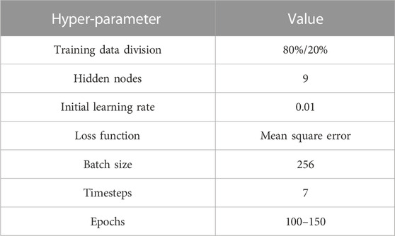
TABLE 1. Hyper-parameters of the LSTM-RN models.
As described in Section 3.1, the data were divided into training and testing sets. Furthermore, a reasonable 20% of the training set was treated as a validation set, which was used to optimize the network parameters during the training process. The number of hidden layer nodes was a key hyperparameter; if it was small, the data characteristics could not be fully retrieved and if it was large, the network’s complexity would increase and eventually overfit. Based on the empirical formula proposed by Xia et al. (2005), nine hidden layer nodes were determined; overfitting or underfitting phenomena were not apparent. The initial learning rate was set to .01, and it gradually decayed during the training process. The batch size determined the frequency with which the weights of the network were updated. It was set to 256 owing to the large amount of data used in this study.
The mean-square error (MSE) was used as the loss of the LSTM-RN models, which decreased with increasing epochs, and the epochs where both validation loss and training loss converged was used as the final epochs. Figure 4 shows the training progress of two randomly selected models, station KOI and EGDM. After training, all the LSTM-RN models in this study converged when the epochs were between 100 and 150. Timesteps was the lengths of the input nodes at a time (Figure 2). The RMSEs of the training sets of all the LSTM-RN models at different time steps were averaged, and the results are shown in Figure 5. In this study, the timesteps of all models were determined to be seven according to the results, while considering the correlation between rainfall periods.
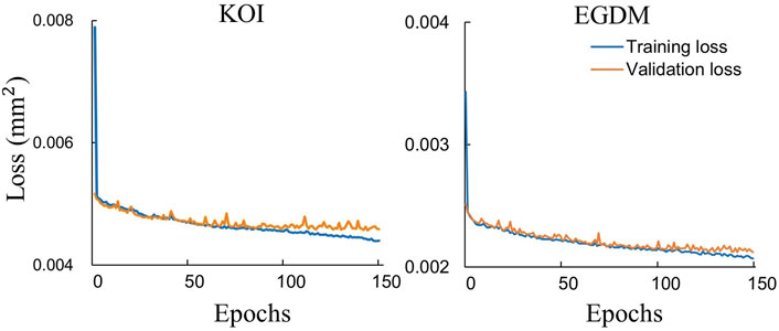
FIGURE 4. Training progress of the LSTM-RN models at stations KOI and EGDM.
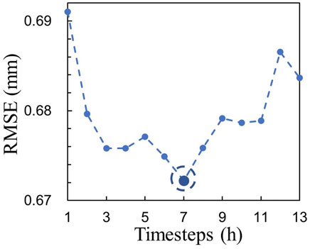
FIGURE 5. Average RMSE of the training sets of all LSTM-RN models at different timesteps.
Error backpropagation algorithms were used to update the parameters of the networks during training. These included stochastic gradient descent (Graves and Schmidhuber, 2005), adaptive gradient (AdaGrad), root mean square prop (RMSProp) (Duchi et al., 2011), and adaptive moment estimation (Adam). The Adam optimization algorithm is an effective gradient-based stochastic optimization method. It combines the advantages of the AdaGrad and RMSProp algorithms to calculate adaptive learning rates for different parameters while using less storage space. It outperformed other stochastic optimization methods in practical applications (Kingma and Ba, 2014); hence, it was used in this study.
For the RF-RN models, the critical parameters were Ntree and Mtry. Ntree represents the number of decision trees (N in Section 3.2). A larger number of decision trees will develop more accurate results, but require more memory. Mtry, the number of input features per leaf node, was usually set to 1/3 of the total number of variables. In our RF-RN models, Ntree was set to 400, according to the out-of-bag error (Figure 6), and Mtry was set to 2. The out-of-bag error served as an indicator of the generalization error, and was used to determine the parameters of an RF model.
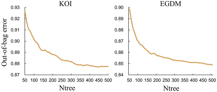
FIGURE 6. The out-of-bag error of the RF-RN models at stations KOI and EGDM.
As rain gauges vary in geographical location, the ability of the LSTM-RN models may be influenced by a variety of environmental conditions. As described in Section 3.4, the RMSE, MBE, and COR of LSTM-RN at different altitudes were calculated. In addition, because the LSTM-RN models have long memory ability and are suitable for multi-step-ahead prediction, three metrics of the models at lead times of 1–6 h were also calculated.
Table 2 shows the RMSE, MBE, and COR of the test sets of the models at different altitudes. It is evident that the RMSE of the low-altitude models was lower than that of the medium- and high-altitude models, possibly because rainfall in low-altitude areas is usually small, so even if the model fails to predict accurately, the results would not significantly deviate from the actual value. However, in medium- and high-altitude areas, where heavy rainfall occurs frequently, the predicted results could deviate more from the real values when the model fails to predict accurately, leading to a high RMSE.
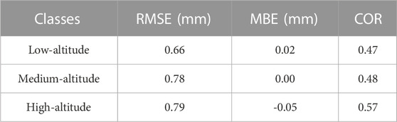
TABLE 2. RMSE, MBE, and COR of the LSTM-RN models at different altitudes.
The MBE of the models was positive at low altitude, zero at middle altitude, and negative at high altitude. It demonstrated that the models showed a tendency to overestimate rainfall at low altitude while underestimating it at high altitude, with the highest variation at high altitude.
The COR of the models between the predicted values and the true values was slightly smaller at low and medium altitudes compared with that at high altitude. The results indicated that the models could perform better when recognizing heavy rainfall trends.
The RMSE, MBE, and COR of the test sets of the LSTM-RN models at different lead times are listed in Table 4. The results revealed that the RMSE increased as the lead time extended, from .72 at 1-h lead time to .77 at 6-h lead time, an increase of 6.94%. The COR decayed with increasing lead time, from .68 at 1-h lead time to .36 at 6-h lead time, a decrease of 47.06%. In general, the performance of the designed models was satisfying, with a slight decay at long lead times.
To assess the performance of the LSTM-RN models, we constructed RF-RN and OF-RN models for comparison. The LSTM-RN and RF-RN models were constructed using radar, gauge rainfall, and atmospheric data, whereas the OF-RN models used only radar rainfall. Four rainfall events were selected from the test sets to visually present the predictive ability of the three types of models at 1-h lead time. To ensure the spatial diversity of the selected events, four randomly selected rainfall events at four stations with large altitude differences were included (see Table 3). The four events almost covered all seasons, with accumulated rainfall ranging from 22.4 mm to 60.4 mm.
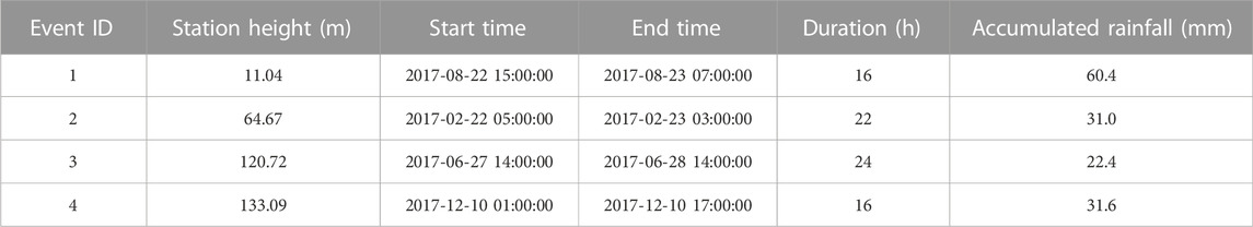
TABLE 3. Durations and accumulated rainfall of selected storm events.
Figure 7 depicts the gauge rainfall and the predicted results using the three types of models for the four rainfall events. Generally, the LSTM-RN models exhibited the best performance compared to the other two models. This was supported by the fact that the LSTM-RN models were able to predict rainfall more accurately at both high and low rainfall rates as well as precisely capture rainfall trends. The performance of the RF-RN model was the second best. They tended to underestimate rainfall at high rainfall rates and overestimate rainfall at low rainfall rates (Figure 7C). However, they could recognize the rainfall trends to some extent. The OF-RN models performed the worst, deviating severely from the gauge rainfall, and sometimes even failing to capture the rainfall trends (Figure 7B).
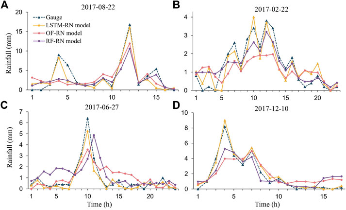
FIGURE 7. The gauge rainfall and the predicted results using three types of models of four rainfall events.
To quantitatively evaluate the prediction performance of the different models, the RMSE, MBE, and COR were calculated at different lead times for the three types of models. Models were categorized into three classes based on altitude, similar to the classification in Section 4.2. Thus, we can compare the performances of the three types of models more easily.
Figure 8 shows the RMSE, MBE, and COR of the three types of models at different lead times and altitudes. In terms of RMSE, it can be seen that the LSTM-RN models performed the best at any lead time and altitude, followed by the RF-RN and OF-RN. As the lead time increased, the RMSE of all models increased, among which the LSTM-RN grew the slowest, followed by RF-RN, while OF-RN grew rapidly. As the altitude increased, the RMSEs of all models also increased, but the LSTM-RN had the smallest gain, while the OF-RN had the largest gain. The results demonstrate that although the accuracy of the models decayed with increasing lead time and altitude, the LSTM-RN models consistently outperformed the others. This may be attributed to the strong memory and excellent learning abilities of LSTM networks, which allow the LSTM-RN to adapted better to changing conditions. The RF-RN models also performed well, with RF being a popular machine-learning method. The OF-RN models, however, showed large errors, especially at longer lead times, owing to a lack of learning ability and reliance solely on the correlation between adjacent frames in the image sequence.
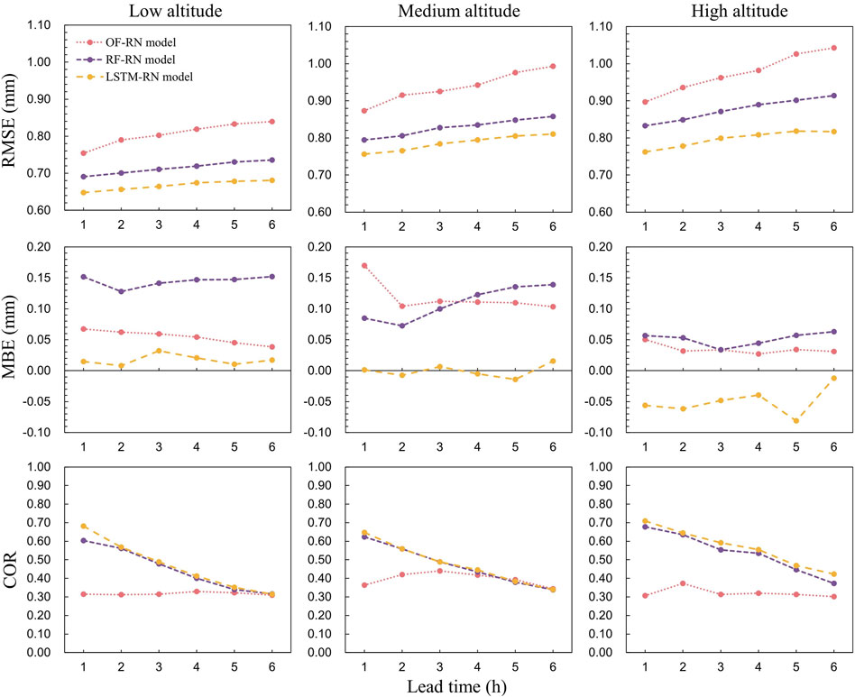
FIGURE 8. Comparison of RMSE, MBE, and COR of three types of models at different lead times and altitudes.
In terms of MBE, it can be seen that LSTM-RN models generally fluctuated around 0 at low and medium altitudes and were <0 at high altitudes. For the other two models, the MBE values were >0 at all altitudes. In other words, the RF-RN and OF-RN models tended to overestimate rainfall compared to LSTM-RN. In general, the LSTM-RN with the minimum deviation performed the best, implying that it rarely overestimated or underestimated rainfall, or the accumulated overestimation and underestimation were virtually equal.
The CORs of the OF-RN were maintained at a low level between .31 and .33, while those of the LSTM-RN and RF-RN decayed with increasing lead time, from ∼.70 to .30. There was no significant difference between the LSTM-RN and RF-RN, except at the 1-h lead time, where the LSTM-RN performed slightly better. In general, both the RF-RN and LSTM-RN performed well at short lead times (1–2 h) with CORs ranging from ∼.50 to .70, and at long lead times (3–6 h) with CORs between ∼.30 and .50. OF-RN was underperforming, with consistently low CORs.
To further compare the performances of the three types of models, we averaged the three metrics for all stations. The RMSE, MBE, and COR of the three types of models at different lead times are listed in Table 4. In terms of RMSE, compared with the OF-RN, the LSTM-RN decreased by 14.15%, 16.72%, 16.45%, 16.98%, 18.80%, and 19.73% at lead times of 1 h–6 h, respectively. Generally, the LSTM-RN decreased by 15.43% at short lead times (1–2 h) and by 17.99% at long lead times (3–6 h). Similarly, compared with that of RF-RN, the RMSE of LSTM-RN decreased by 6.52%, 6.60%, 6.73%, 6.80%, 7.22%, and 7.96% at lead times of 1–6 h, respectively. The RMSE of the LSTM-RN decreased by 6.56% at short lead times (1–2 h) and by 7.17% at long lead times (3–6 h). In other words, although the prediction accuracy of the three types of models decreased as lead time increased, the LSTM-RN with strong learning and memory ability performed best, with the lowest RMSEs at any given lead time, and a growing advantage at longer lead times.
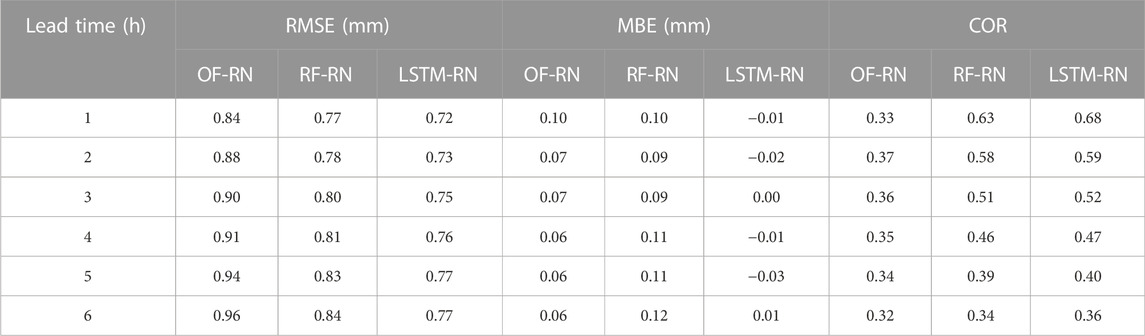
TABLE 4. RMSE, MBE, and COR of three types of models at different lead times.
In terms of COR, compared with the OF-RN, the LSTM-RN increased by 106.99%, 60.41%, 47.21%, 32.62%, 17.15%, and 12.72% at lead times of 1 h–6 h, respectively, with an average of 46.18%. Similarly, compared with the RF-RN, the LSTM-RN increased by 7.04%, .98%, 3.20%, 3.06%, 3.48%, and 4.80% at lead times of 1 h–6 h, respectively, with an average of 3.76%. In general, the OF-RN did not perform satisfactorily in capturing the rainfall trends, and both the RF-RN and LSTM-RN performed well, with the LSTM-RN showing a slight advantage.
In Section 4.2, the performance of the LSTM-RN model at different lead times and altitudes was discussed, and it was apparent that model performance displayed regular patterns at different altitudes. Since altitude is highly relevant to weather conditions, this study investigated the relationship between LSTM-RN models and weather conditions. Through pre-experiments, we discovered that the model performance was related to rainfall rates and relative humidity; therefore, we focused on these two factors to further evaluate the model performance under various weather conditions.
As described in Section 3.4, the test sets were divided into five classes based on rainfall rate, and three metrics (RMSE, relative bias, and COR) were calculated. Similar to the division in Section 4.2, the models were divided into three classes based on altitude, and the metrics were averaged for each class of models.
Figure 9A shows the RMSE, relative bias, and COR of the three classes of models at different rainfall rates. The blue, yellow, and orange lines represent the low-altitude, medium-altitude, and the high-altitude models, respectively. It can be clearly observed that the curves are highly similar in terms of altitude. The RMSE generally increased as the rainfall rate increased, from ∼.40 to 2.00. We noted that the smallest rainfall rate (A1) did not correspond to the lowest RMSE, that is, light rain was more difficult to predict accurately than moderate rain (A2–A3). Furthermore, the relative bias of light rain (A1) was more pronounced than that of heavy rain (A5–A6). In addition, COR increased as the rainfall rate increased, which is consistent with the explanation in Section 4.2.
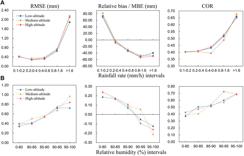
FIGURE 9. RMSE, relative bias (MBE), and COR of three classes of models at different rainfall rate and relative humidity, respectively.
As the atmospheric factors are complicated, this study selected temperature, relative humidity, and wind speed for pre-experiments and discovered that relative humidity showed an obvious correlation with the model performance. Figure 9B shows the RMSE, MBE, and COR of the three classes of models at different relative humidities. As relative humidity increased, the RMSE increased from ∼.40 to .80, the MBE decreased from ∼.20 to –.20, and the COR increased from ∼.40 to .70. The results demonstrated that the models showed low RMSEs at low relative humidity, low bias at medium relative humidity, and high CORs at high relative humidity.
As the results show a similar tendency in terms of altitude (Figure 9), error metrics were averaged at different rainfall rate and relative humidity classes, excluding the altitude (Tables 5, 6). The results revealed that the RMSE improved by 388.10% from A1 to A5 and by 123.68% from B1 to B5. COR improved by 65% from A1 to A5 and by 72.50% from B1 to B5. In general, the models showed a higher accuracy under light rain and low relative humidity, lower uncertainty under moderate rain and medium relative humidity, and better recognition of rainfall trends under heavy rain and high relative humidity.
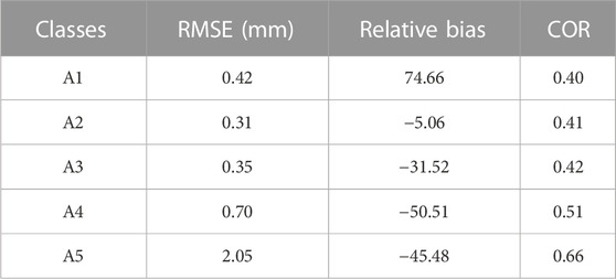
TABLE 5. Comparison of RMSE, relative bias, and COR among the five rainfall rate classes (A1–A5).
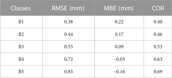
TABLE 6. Comparison of RMSE, MBE, and COR among the five relative humidity classes (B1–B5).
Although the proposed LSTM-RN models achieved reasonable performance, the prediction at stations still has limitations. In future work, meteorological forecast fields, such as the European Centre for Medium-Range Weather Forecasts (ECMWF), the global forecast system from China T639, and the National Centers for Environmental Prediction (NCEP) Global Forecast System (GFS), will be employed to investigate regional predictions (Li et al., 2021). Using these data for radar nowcasting could produce more accurate and practical results over precipitation areas.
In this study, we constructed radar rainfall nowcasting models using LSTM networks, with radar rainfall data as input and rain gauge data as ground references. To correct radar estimate errors and improve the nowcasting ability under various weather conditions, atmospheric data were also used as input. The 40 scattered stations used for modeling roughly represented the various environments of the study area. Approximately 11 years of data from the stations were employed as training and test sets to confirm its adequacy. After adjusting the hyperparameters, we determined the optimal settings for all stations. The performance of the LSTM-RN was evaluated at various lead times and altitudes and was compared with that of the OF-RN and RF-RN. We also investigated the relationship between the performance of the LSTM-RN and weather conditions. The results are summarized as follows:
(1) The performance of LSTM-RN displayed regular patterns at different altitudes. The RMSEs of the models at high altitudes were generally higher than those at low altitudes; however, the CORs were also generally higher at high altitudes. Moreover, models at high altitudes tended to underestimate rainfall, while models at low altitudes tended to overestimate rainfall, with the highest variation at high altitudes.
(2) Compared with OF-RN and RF-RN, LSTM-RN demonstrated the highest accuracy in nowcasting, with the lowest RMSEs and MBEs closest to 0 at any lead time. Furthermore, the LSTM-RN had a growing advantage in longer lead times, with the RMSE decreasing by 15.43% and 6.56% at short lead times (1–2 h) and by 17.99% and 7.17% at long lead times (3–6 h). In addition, the LSTM-RN significantly outperformed the others in recognizing rainfall trends, with the highest CORs at any given lead time. On average, the COR of the LSTM-RN increased by 46.18% and 3.76%, compared with that of the OF-RN and RF-RN, respectively.
(3) A strong relationship between the performance of the LSTM-RN and weather conditions was observed. The models showed a higher accuracy under light rain and low relative humidity, lower uncertainty under moderate rain and medium relative humidity, and better recognition of rainfall trends under heavy rain and high relative humidity.
This study proposes a reliable and effective solution to nowcast radar rainfall at long lead times using an advanced deep learning technique, as well as considering the atmospheric impact on radar data. The results demonstrate that the designed models outperform traditional methods in prediction ability and are valuable for long lead-time nowcasting. However, owing to data limitations and the computational expenses for model training, this study can only realize nowcasting on stations. In future work, we intend to collect gauge data from more stations to achieve regional nowcasting.
The original contributions presented in the study are included in the article/supplementary material, further inquiries can be directed to the corresponding author.
Conceptualization, KZ and QY; Methodology, KZ, QY, SZ, and YY; Validation, SJ, TW, and JL; Formal analysis, KZ and SJ; Investigation, KZ, TW, and JL; Data cura-tion, SJ; Writing—original draft preparation, KZ; Writing—review and editing, KZ and QY; Visualization, KZ; Supervision, SZ. All authors have read and agreed to the published version of the manuscript.
This study was supported by the National Natural Science Foundation of China (Nos. 42271483, 42101416, and 42071364).
The authors declare that the research was conducted in the absence of any commercial or financial relationships that could be construed as a potential conflict of interest.
All claims expressed in this article are solely those of the authors and do not necessarily represent those of their affiliated organizations, or those of the publisher, the editors and the reviewers. Any product that may be evaluated in this article, or claim that may be made by its manufacturer, is not guaranteed or endorsed by the publisher.
Agrawal, S., Barrington, L., Bromberg, C., Burge, J., Gazen, C., and Hickey, J. (2019). Machine learning for precipitation nowcasting from radar images. arXiv e-prints, arXiv:1912.12132.
Ayzel, G., Heistermann, M., and Winterrath, T. (2019). Optical flow models as an open benchmark for radar-based precipitation nowcasting (rainymotion v0.1). Geosci. Model Dev. 12 (4), 1387–1402. doi:10.5194/gmd-12-1387-2019
Ayzel, G., Scheffer, T., and Heistermann, M. (2020). RainNet v1.0: A convolutional neural network for radar-based precipitation nowcasting. Geosci. Model Dev. 13 (6), 2631–2644. doi:10.5194/gmd-13-2631-2020
Berenguer, M., Sempere-Torres, D., and Pegram, G. G. S. (2011). SBMcast – an ensemble nowcasting technique to assess the uncertainty in rainfall forecasts by Lagrangian extrapolation. J. Hydrology 404 (3-4), 226–240. doi:10.1016/j.jhydrol.2011.04.033
Bowler, N. E. H., Pierce, C. E., and Seed, A. (2004). Development of a precipitation nowcasting algorithm based upon optical flow techniques. J. Hydrology 288 (1-2), 74–91. doi:10.1016/j.jhydrol.2003.11.011
Buehner, M., and Jacques, D. (2020). Non-Gaussian deterministic assimilation of radar-derived precipitation accumulations. Mon. Weather Rev. 148 (2), 783–808. doi:10.1175/MWR-D-19-0199.1
Chen, S., Adjei, C. O., Tian, W., Onzo, B.-M., Kedjanyi, E. A. G., and Darteh, O. F. (2021). Rainfall forecasting in sub-sahara africa-Ghana using LSTM deep learning approach. Int. J. Eng. Res. Technol. 10 (3), 464–470. doi:10.17577/IJERTV10IS030244
Cuo, L., Pagano, T. C., and Wang, Q. J. (2011). A review of quantitative precipitation forecasts and their use in short- to medium-range streamflow forecasting. J. Hydrometeorol. 12 (5), 713–728. doi:10.1175/2011JHM1347.1
Dai, Q., and Han, D. (2014). Exploration of discrepancy between radar and gauge rainfall estimates driven by wind fields. Water Resour. Res. 50 (11), 8571–8588. doi:10.1002/2014wr015794
Dixon, M., and Wiener, G. (1993). Titan: Thunderstorm identification, tracking, analysis, and nowcasting—a radar-based methodology. J. Atmos. Ocean. Technol. 10 (6), 785–797. doi:10.1175/1520-0426(1993)010<0785:ttitaa>2.0.co;2
Duchi, J., Hazan, E., and Singer, Y. (2011). Adaptive subgradient methods for online learning and stochastic optimization. J. Mach. Learn. Res. 12 (7), 2121–2159.
Ebert, E. E., Wilson, L. J., Brown, B. G., Nurmi, P., Brooks, H. E., Bally, J., et al. (2004). Verification of nowcasts from the WWRP sydney 2000 forecast demonstration project. Weather Forecast. 19 (1), 73–96. doi:10.1175/1520-0434(2004)019<0073:vonftw>2.0.co;2
Foresti, L., Sideris, I. V., Nerini, D., Beusch, L., and Germann, U. (2019). Using a 10-year radar archive for nowcasting precipitation growth and decay: A probabilistic machine learning approach. Weather Forecast. 34 (5), 1547–1569. doi:10.1175/WAF-D-18-0206.1
Gers, F. A., Schraudolph, N. N., and Schmidhuber, J. (2002). Learning precise timing with LSTM recurrent networks. J. Mach. Learn. Res. 3, 115–143. doi:10.1162/153244303768966139
Golding, B. W. (1998). Nimrod: A system for generating automated very short range forecasts. Meteorol. App. 5 (1), S1350482798000577. doi:10.1017/S1350482798000577
Graves, A., and Schmidhuber, J. (2005). Framewise phoneme classification with bidirectional LSTM and other neural network architectures. Neural Netw. 18 (5-6), 602–610. doi:10.1016/j.neunet.2005.06.042
Grecu, M., and Krajewski, W. F. (2000). A large-sample investigation of statistical procedures for radar-based short-term quantitative precipitation forecasting. J. Hydrology 239 (1), 69–84. doi:10.1016/S0022-1694(00)00360-7
Hernández, E., Sanchez-Anguix, V., Julian, V., Palanca, J., and Duque, N. (2016). “Rainfall prediction: A deep learning approach,” in Hybrid artificial intelligent systems. Editors F. Martínez-Álvarez, A. Troncoso, H. Quintián, and E. Corchado (New York: Springer International Publishing), 151–162.)
Hochreiter, S., and Schmidhuber, J. (1997). Long short-term memory. Neural Comput. 9 (8), 1735–1780. doi:10.1162/neco.1997.9.8.1735
Imhoff, R. O., Brauer, C. C., Overeem, A., Weerts, A. H., and Uijlenhoet, R. (2020). Spatial and temporal evaluation of radar rainfall nowcasting techniques on 1, 533 events. Water Resour. Res. 56 (8). doi:10.1029/2019wr026723
Jia, Y., Wu, J., and Xu, M. (2017). Traffic flow prediction with rainfall impact using a deep learning method. J. Adv. Transp. 2017, 1–10. doi:10.1155/2017/6575947
Joss, J., and Lee, R. (1995). The application of radar–gauge comparisons to operational precipitation profile corrections. J. Appl. Meteor. 34 (12), 2612–2630. doi:10.1175/1520-0450(1995)034<2612:taorct>2.0.co;2
Kang, J., Wang, H., Yuan, F., Wang, Z., Huang, J., and Qiu, T. (2020). Prediction of precipitation based on recurrent neural networks in jingdezhen, jiangxi province, China. Atmosphere 11 (3), 246. doi:10.3390/atmos11030246
Kingma, D. P., and Ba, J. (2014). Adam: A method for stochastic optimization. arXiv e-prints, arXiv:1412.6980.
Koizumi, K. (1999). An objective method to modify numerical model forecasts with newly given weather data using an artificial neural network. Weather Forecast. 14 (1), 109–118. doi:10.1175/1520-0434(1999)014<0109:aomtmn>2.0.co;2
Krämer, S., Verworn, H. R., and Redder, A. (2005). Improvement of X-band radar rainfall estimates using a microwave link. Atmos. Res. 77 (1-4), 278–299. doi:10.1016/j.atmosres.2004.10.028
Kroeger, T., Timofte, R., Dai, D., and Van Gool, L. (2016). “Fast optical flow using dense inverse search,” in Computer vision – eccv 2016. Editors B. Leibe, J. Matas, N. Sebe, and M. Welling (New York: Springer International Publishing), 471–488.
Kumar, A., Islam, T., Sekimoto, Y., Mattmann, C., and Wilson, B. (2020). Convcast: An embedded convolutional LSTM based architecture for precipitation nowcasting using satellite data. Plos one 15 (3), e0230114. doi:10.1371/journal.pone.0230114
Le, J. A., El-Askary, H. M., Allali, M., and Struppa, D. C. (2017). Application of recurrent neural networks for drought projections in California. Atmos. Res. 188, 100–106. doi:10.1016/j.atmosres.2017.01.002
Li, X., Yang, Y., Mi, J., Bi, X., Zhao, Y., Huang, Z., et al. (2021). Leveraging machine learning for quantitative precipitation estimation from Fengyun-4 geostationary observations and ground meteorological measurements. Atmos. Meas. Tech. 14 (11), 7007–7023. doi:10.5194/amt-14-7007-2021
Liguori, S., and Rico-Ramirez, M. A. (2013). A review of current approaches to radar-based quantitative precipitation forecasts. Int. J. River Basin Manag. 12 (4), 391–402. doi:10.1080/15715124.2013.848872
Liguori, S., Rico-Ramirez, M. A., Schellart, A. N. A., and Saul, A. J. (2012). Using probabilistic radar rainfall nowcasts and NWP forecasts for flow prediction in urban catchments. Atmos. Res. 103, 80–95. doi:10.1016/j.atmosres.2011.05.004
Liu, Y., Xi, D.-G., Li, Z.-L., and Hong, Y. (2015). A new methodology for pixel-quantitative precipitation nowcasting using a pyramid Lucas Kanade optical flow approach. J. Hydrology 529, 354–364. doi:10.1016/j.jhydrol.2015.07.042
Lucas, B. D., and Kanade, T. (1981). “An iterative image registration technique with an application to stereo vision,” in Proceedings of the 7th international joint conference on Artificial intelligence - Volume 2, Vancouver, BC, Canada, August 24 - 28, 1981 (Morgan Kaufmann Publishers Inc.).
Luo, C., Li, X., and Ye, Y. (2020). PFST-LSTM: A spatiotemporal LSTM model with pseudoflow prediction for precipitation nowcasting. IEEE J. Sel. Top. Appl. Earth Obs. Remote Sens. 14, 843–857. doi:10.1109/jstars.2020.3040648
Milewski, A., Elkadiri, R., and Durham, M. (2015). Assessment and comparison of TMPA satellite precipitation products in varying climatic and topographic regimes in Morocco. Remote Sens. 7 (5), 5697–5717. doi:10.3390/rs70505697
Met Office (2019). MIDAS Open: UK hourly weather observation data, v201901. Centre for Environmental Data Analysis. March, 01, 2019. doi:10.5285/c58c1af69b9745fda4cdf487a9547185
Pierce, C., Seed, A., Ballard, S., Simonin, D., and Li, Z. (2012). Doppler radar observations: Weather radar, wind profiler, ionospheric radar, and other advanced applications. London: IntechOpen, 97–142.
Pulkkinen, S., Nerini, D., Pérez Hortal, A. A., Velasco-Forero, C., Seed, A., Germann, U., et al. (2019). Pysteps: An open-source Python library for probabilistic precipitation nowcasting (v1.0). Geosci. Model Dev. 12 (10), 4185–4219. doi:10.5194/gmd-12-4185-2019
Ravuri, S., Lenc, K., Willson, M., Kangin, D., Lam, R., Mirowski, P., et al. (2021). Skilful precipitation nowcasting using deep generative models of radar. Nature 597 (7878), 672–677. doi:10.1038/s41586-021-03854-z
Schmidhuber, J. (2015). Deep learning in neural networks: An overview. Neural Netw. 61, 85–117. doi:10.1016/j.neunet.2014.09.003
Seo, D. J., Breidenbach, J. P., and Johnson, E. R. (1999). Real-time estimation of mean field bias in radar rainfall data. J. Hydrology 223 (3), 131–147. doi:10.1016/S0022-1694(99)00106-7
Shi, X., Chen, Z., Wang, H., Yeung, D.-Y., Wong, W.-K., and Woo, W.-c. (2015). “Convolutional LSTM network: A machine learning approach for precipitation nowcasting,” in Advances in neural information processing systems, Montreal Canada, December 7 - 12, 2015.28
Shi, X., Gao, Z., Lausen, L., Wang, H., Yeung, D.-Y., Wong, W.-k., et al. (2017). “Deep learning for precipitation nowcasting: A benchmark and a new model,” in Advances in neural information processing systems, Long Beach California USA, December 4 - 9, 2017.30
Song, Y., Han, D., and Zhang, J. (2017). Radar and rain gauge rainfall discrepancies driven by changes in atmospheric conditions. Geophys. Res. Lett. 44 (14), 7303–7309. doi:10.1002/2017gl074493
Speiser, J. L., Miller, M. E., Tooze, J., and Ip, E. (2019). A comparison of random forest variable selection methods for classification prediction modeling. Expert Syst. Appl. 134, 93–101. doi:10.1016/j.eswa.2019.05.028
Sun, J. (2005). Convective-scale assimilation of radar data: Progress and challenges. Q. J. R. Meteorol. Soc. 131 (613), 3439–3463. doi:10.1256/qj.05.149
Sun, J., Xue, M., Wilson, J. W., Zawadzki, I., Ballard, S. P., Onvlee-Hooimeyer, J., et al. (2014). Use of NWP for nowcasting convective precipitation: Recent progress and challenges. Bull. Am. Meteorol. Soc. 95 (3), 409–426. doi:10.1175/bams-d-11-00263.1
Sun, P., Ma, Z., Zhang, Q., Singh, V. P., and Xu, C.-Y. (2022). Modified drought severity index: Model improvement and its application in drought monitoring in China. J. Hydrol. 612, 128097.
Tian, L., Li, X., Ye, Y., Xie, P., and Li, Y. (2019). A generative adversarial gated recurrent unit model for precipitation nowcasting. IEEE Geosci. Remote Sens. Lett. 17 (4), 601–605. doi:10.1109/lgrs.2019.2926776
Valverde Ramírez, M. C., de Campos Velho, H. F., and Ferreira, N. J. (2005). Artificial neural network technique for rainfall forecasting applied to the São Paulo region. J. Hydrology 301 (1), 146–162. doi:10.1016/j.jhydrol.2004.06.028
Van, S. P., Le, H. M., Thanh, D. V., Dang, T. D., Loc, H. H., and Anh, D. T. (2020). Deep learning convolutional neural network in rainfall–runoff modelling. J. Hydroinformatics 22 (3), 541–561. doi:10.2166/hydro.2020.095
Vila, D. A., Machado, L. A. T., Laurent, H., and Velasco, I. (2008). Forecast and tracking the evolution of cloud clusters (ForTraCC) using satellite infrared imagery: Methodology and validation. Weather Forecast. 23 (2), 233–245. doi:10.1175/2007waf2006121.1
Villarini, G., and Krajewski, W. F. (2009). Review of the different sources of uncertainty in single polarization radar-based estimates of rainfall. Surv. Geophys. 31 (1), 107–129. doi:10.1007/s10712-009-9079-x
Warner, B., and Misra, M. (1996). Understanding neural networks as statistical tools. Am. Statistician 50 (4), 284–293. doi:10.1080/00031305.1996.10473554
Wilson, J. W., Feng, Y., Chen, M., and Roberts, R. D. (2010). Nowcasting challenges during the beijing olympics: Successes, failures, and implications for future nowcasting systems. Weather Forecast. 25 (6), 1691–1714. doi:10.1175/2010waf2222417.1
Woo, W.-c., and Wong, W.-k. (2017). Operational application of optical flow techniques to radar-based rainfall nowcasting. Atmosphere 8 (12), 48. doi:10.3390/atmos8030048
Wang, Y., Coning, E. D., Harou, A., Jacobs, W., Joe, P., Nikitina, L., et al. (2017). Guidelines for nowcasting techniques. Available at: public.wmo.int/en/resources/bulletin/nowcasting-guidelines-%E2%80%93-summary (Accessed December 3, 2022).
Xia, K.-W., Li, C.-B., and Shen, J.-Y. (2005). An optimization algorithm on the number of hidden layer nodes in feed-forward neural network. Comput. Sci. 32 (10), 143–145.
Yang, Q., Dai, Q., Han, D., Zhu, Z., and Zhang, S. (2020). Uncertainty analysis of radar rainfall estimates induced by atmospheric conditions using long short-term memory networks. J. Hydrology 590, 125482. doi:10.1016/j.jhydrol.2020.125482
Zahraei, A., Hsu, K.-l., Sorooshian, S., Gourley, J. J., Hong, Y., and Behrangi, A. (2013). Short-term quantitative precipitation forecasting using an object-based approach. J. Hydrology 483, 1–15. doi:10.1016/j.jhydrol.2012.09.052
Keywords: nowcasting, radar, rainfall, atmospheric conditions, deep learning, long short-term memory
Citation: Zhu K, Yang Q, Zhang S, Jiang S, Wang T, Liu J and Ye Y (2023) Long lead-time radar rainfall nowcasting method incorporating atmospheric conditions using long short-term memory networks. Front. Environ. Sci. 10:1054235. doi: 10.3389/fenvs.2022.1054235
Received: 26 September 2022; Accepted: 28 November 2022;
Published: 20 January 2023.
Edited by:
Zengyun Hu, Chinese Academy of Sciences (CAS), ChinaReviewed by:
Aihong Cui, Hong Kong Baptist University, Hong Kong SAR, ChinaCopyright © 2023 Zhu, Yang, Zhang, Jiang, Wang, Liu and Ye. This is an open-access article distributed under the terms of the Creative Commons Attribution License (CC BY). The use, distribution or reproduction in other forums is permitted, provided the original author(s) and the copyright owner(s) are credited and that the original publication in this journal is cited, in accordance with accepted academic practice. No use, distribution or reproduction is permitted which does not comply with these terms.
*Correspondence: Shuliang Zhang, emhhbmdzaHVsaWFuZ0Buam51LmVkdS5jbg==
Disclaimer: All claims expressed in this article are solely those of the authors and do not necessarily represent those of their affiliated organizations, or those of the publisher, the editors and the reviewers. Any product that may be evaluated in this article or claim that may be made by its manufacturer is not guaranteed or endorsed by the publisher.
Research integrity at Frontiers
Learn more about the work of our research integrity team to safeguard the quality of each article we publish.