Road grade estimation for vehicle emissions modeling using electronic atmospheric pressure sensors

Vehicle specific power (VSP) is useful for estimation of vehicle emissions. Previous research has indicated that vehicle specific power and emissions are sensitive to variation of road grade. Several methods have been used for acquisition of road grade data in earlier studies, but all have certain limitations such as insufficient accuracy, complicated data processing, or requirements for devices or data that are not easily available. The objective of this study was to develop and verify a road grade measurement framework based on an electronic pressure sensor. The method includes atmospheric pressure acquisition using electronic sensors, determination of the pressure-altitude relationship based on meteorological station data, filtering of altitude data by Fourier transform, and grade calculation combined with the onboard diagnostics distance. Road grades and vehicle specific power calculated based on atmospheric pressure were found reliable and accurate, which also improved the accuracy of vehicle emission rates calculation.

GRAPHICAL ABSTRACT

1 Introduction

Vehicle specific power (VSP), which is useful for estimation of vehicle emissions, is the instantaneous power per unit mass of the vehicle calculated based on its speed and acceleration and the road grade (Jimenz-Palacios, 1999; Frey et al., 2002; Nam, 2003). It accounts for the power demand, rolling resistance, and road grade, and has been used to develop empirical models of light-duty vehicle emissions based on second-by-second dynamometer and portable emissions measurement system (PEMS) data (EPA, 2002). Previous research has indicated that VSP and emissions are sensitive to variation of road grade (Denis and Winer, 1993; Enns et al., 1993; Kelly and Groblicki, 1993; Denis et al., 1994; Pierson et al., 1996; Cicero-Fernandez et al., 1997; Rosero et al., 2021). For a given speed, larger positive road grades lead to increased VSP, which in turn leads to higher average emission rates. For example, the estimated average NO emission rate for a road grade of 6% is approximately a factor of two greater than that for a 0% road grade (Zhang and Frey, 2012). Therefore, precise grade data are important for VSP calculation and emissions estimation.

The measurement of road grade is more difficult than the calculation of speed and acceleration, precise measurements of which can be obtained directly from the electronic control unit (ECU) of a vehicle using the onboard diagnostics (OBD) protocol. In previous research (Souleyrette et al., 2003; Toutin, 2004; Zhang and Frey, 2012; Zhang et al., 2021, 2019; Perugu, 2019; Chong et al., 2020), although several different methods have been used for acquisition of road grade data, for example, design drawing data, traditional surveying, GPS measurements, and mobile mapping such as LiDAR, all have certain limitations in their application.

Design drawing data can be convenient for inferring the road grade of a corresponding roadway. However, owing to the potential for errors and changes during construction, road grades estimated from design drawing data might not be sufficiently accurate. Furthermore, obtaining design drawing data often requires authorization from corresponding agencies, and design drawings of different roads might have to be sourced from different agencies, which could complicate the data acquisition process.

Traditional surveying using various devices (e.g., a rangefinder or total station) can provide relatively precise grade data by measuring distances and vertical height differences. However, data collection using this method can be a time-consuming and expensive process. Furthermore, the measurements should be performed on the road of interest, which means it can be dangerous because it is often unrealistic to expect to close roadways to ensure measurement safety. Use of a digital inclinometer in a moving vehicle is another direct on-road method for obtaining road grade data. However, the vehicle’s suspension system can mean that measurements of the body angle of the vehicle do not accurately reflect the grade of the road surface.

GPS measurement is the method used most widely for determining road grade measurements for use in VSP calculations (Awuah-Bzezinska et al., 1997; Bae et al., 2001; Souleyrette et al., 2003). A GPS system can be easily integrated into a PEMS to collect three-dimensional coordinates that can characterize a route. The road grade can then be calculated based on differences of distance and altitude. However, large numbers of buildings along a road could interfere with the GPS signal and affect the accuracy of the GPS measurement results, especially the accuracy of altitude measurements. Undertaking multiple runs along the same roadway and using many other sources of data (Yazdani Boroujeni and Frey, 2014) (e.g., accelerometers and gyroscopes) could improve the accuracy of estimations of road grade. However, such an approach is time consuming and expensive when collecting data over large areas.

Real-time kinematic positioning (RTK), using measurements of the phase of the signal’s carrier wave relies on a single reference station or interpolated virtual station to provide real-time corrections for errors in navigation systems such as GPS (Wanninger, 2018), can provide cm-level accuracy for road grade measurement. However, its limitations are that specialized mapping skills are required to conduct RTK measurement, and a base station or additional fees for RTK network service is necessary. Meanwhile, the measurement accuracy may be impacted by the urban building to a certain extend.

Mobile mapping, such as LiDAR, using a moving platform can integrate data from multiple sensors to provide three-dimensional positioning of both the platform and the ground surface. LiDAR can be used to generate a digital elevation model with cm-level accuracy, which could be used to calculate road grade (Zhang et al., 2003; Toutin, 2004; Liu, et al., 2019). However, this method also has many limitations. For example, owing to the complexity of the land surface of many urban areas attributable to vegetation, buildings, and on-road vehicles, the elevation data obtained might not fully represent reality (Bindschadler et al., 1999; Hill et al., 2000; Sun and Ranson, 2000; Letsky et al., 2002; Hernandez-Pajares et al., 2003; Lim et al., 2003; North Carolina Floodplain Mapping Program, 2013). Moreover, urban areas often have many undercrossing tunnels that prohibit the determination of road grade using LiDAR. The expense of devices such as LiDAR and the time-consuming data processing requirements are other important issues that limit application of this method (Zhang and Frey, 2012). However, with the development of LiDAR, its cost is gradually decreasing, and now it has been widely used in autonomous vehicles. Therefore, the cost of road grade measurements using LiDAR may be reduced in the future.

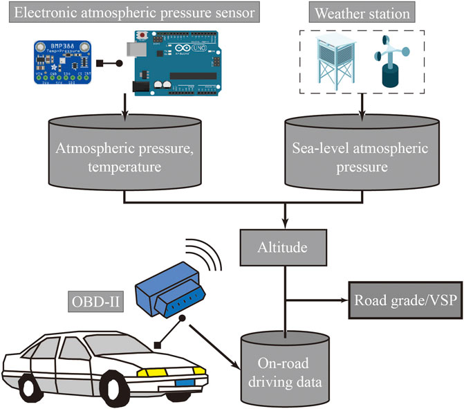
In summary, the above road grade measurement methods all have certain limitations such as insufficient accuracy, complicated data processing, or requirements for devices or data that are not easily available. Therefore, a new method for precise and convenient estimation of road grade is necessary. Generally, owing to specific atmospheric properties, a strong relationship exists between atmospheric pressure and altitude within a certain range. Thus, altitude can be calculated based on atmospheric pressure (World Meteorological Organization, 2007; Keisan, 2018), and road grade can be calculated based on altitude variation. This method of estimation based on altitude already has various applications in the fields of outdoor activities and aviation.

With recent developments in electronic technology, low-cost, high-precision atmospheric pressure sensors (BOSCH, 2015; BOSCH, 2018) provide the possibility of using this method for road grade measurements. By collecting atmospheric pressure data using a low-cost atmospheric pressure sensor and building the relationship between altitude and atmospheric pressure, altitude and road grade data could be calculated precisely. Compare with other methods, the pressure sensor-based method may be slightly less accurate than LiDAR and RTK. However, it is more cost-effective while requiring less equipment and data processing, and it is more convenience and flexible to be conduct in on-road measurement. A Comparison of several methods of road grade measurement were shown in Table 1.

TABLE 1

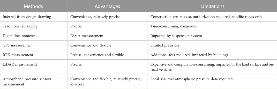
TABLE 1. Comparison of several methods of road grade measurement.

The objectives of this study were to build and verify a road grade measurement framework based on an electronic pressure sensor, and to use the obtained road grade data in calculations of VSP and estimations of emission rates.

2 Methodologies

The methodological approaches used in this study can be divided into two elements: experimental design, and application to VSP and emission rate calculations. In this section, the experimental design is introduced, including descriptions of the devices used in this research, measurement route, data collection and analysis, and verification of the results. Then, the road grade information based on the atmospheric pressure sensor data is used in the calculations of VSP and emission rates to validate the effectiveness of the approach.

2.1 Experimental design

2.1.1 Devices used in this study

The measurement devices used in this study are illustrated in Figure 1 and described in the following.

FIGURE 1

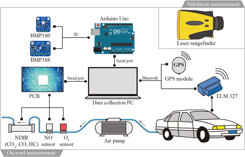
FIGURE 1. Measurement devices used in the study.

The pressure sensors are used for measurement of on-road atmospheric pressure and air temperature. Two types of atmospheric pressure sensor are used in the system: BMP180 and BMP388 (BOSCH, 2015; BOSCH, 2018), for which the absolute accuracy and relative accuracy of the pressure measurements are 1 and 0.4 hPa, and 0.12 and 0.08 hPa, respectively. The accuracy of temperature measurements by the BMP180 and BMP388 sensors is 1.0 and 0.5°C, respectively. The operating temperature of the sensors is −40–85°C, and the measurement range is 300–1,250 hPa, which can well meet the measurement needs. The two sensors are connected to the Arduino Uno (Arduino, 2020) through a IIC interface, and further connected to the data collection PC via a USB serial port.

The atmospheric pressure sensors used in this study were taken to several national meteorological stations within Chengdu (Sichuan Province, China) to obtain comparative measurements. Because there is an error in the measurement results of the atmospheric pressure sensors, and because the meteorological stations only release hourly data, the sensors were used to measure atmospheric pressure within 1 min before the release of the meteorological station data, and the average value was calculated as the measurement result. Table 2 compares the atmospheric pressure published by certain national meteorological stations and that recorded by the electronic atmospheric pressure sensors. The absolute deviation of the measured value acquired by the BMP180 sensor does not exceed 1 hPa and that of the BMP388 sensor does not exceed 0.4 hPa relative to the value published by the national meteorological stations. The relative deviation of the measurements obtained by the BMP180 and BMP388 sensors is <0.05 and <0.01 h Pa, respectively. The results indicate that the values measured using the electronic atmospheric pressure sensors effectively reflect the actual atmospheric pressure value, and that the sensors have an accurate response to relative variations of pressure.

TABLE 2

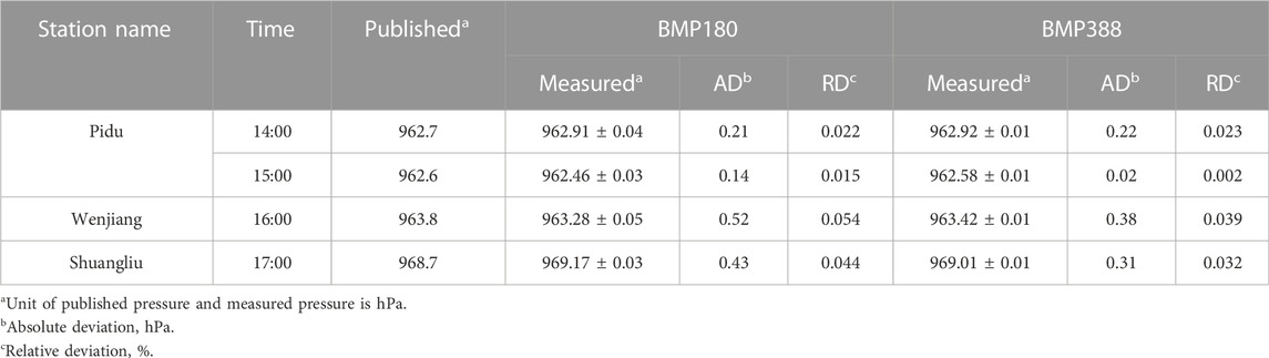
TABLE 2. Comparison of atmospheric pressure published by national meteorological stations and measured by atmospheric pressure sensors (8 December 2019).

The OBD-II interface (ELM Electronics, 2020) is used to connect the ECU of the measured vehicle and for reading the vehicle’s on-road driving parameters, such as speed and engine RPM. The data are transferred via Bluetooth to the data collection PC.

The GPS module is used to collect GPS locations and to transfer the data to the data collection PC via Bluetooth.

The laser rangefinder (TruPulse 200) (LaserTec, 2020) can measure straight-line distance by sending and receiving a laser pulse. The device has a built-in gyroscope, which can obtain the viewing angle and decompose the measured straight-line distance into horizonal distance and vertical distance. The maximum operating distance of the laser rangefinder is 2,000 m, and the accuracy is 0.2 m. The laser rangefinder was used to measure the grade of the validation section of the measurement route to verify the road grade data obtained using the atmospheric pressure sensors and GPS.

2.1.2 Measurement route

The measurement route is shown in Figure 2. The route has overall distance of approximately 30 km, and it includes seven overpasses and five undercrossing tunnels. As marked in Figure 2, a section of the route was selected as the validation section for the laser rangefinder measurements, and the road grade data of this section obtained using different methods were compared for accuracy verification.

FIGURE 2

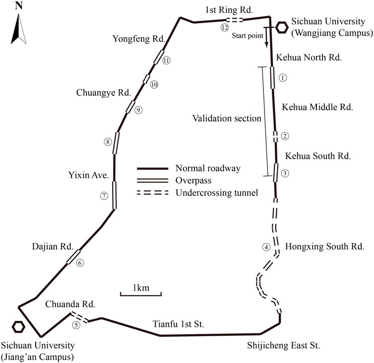
FIGURE 2. On-road measurement route and validation section.

2.1.3 Data collection and analysis

This study conducted two measurement experiments. In the first experiment, the distance and relative altitude of the verification section were measured using the laser rangefinder. Those data were used to calculate the slope data of the verification section as a verification reference. In the second experiment, a car was required to travel along the route. The pressure sensors, OBD interface, GPS module, and gas analysis module were carried onboard the vehicle to collect second-by-second data, which were then used for calculation of the slope along the entire route, and subsequent calculations of VSP and emission rates. The specific details are introduced in the following.

2.1.3.1 Validation data collection and analysis

Although it is time consuming to directly measure road grade, the accuracy of such an approach is reasonably high. Therefore, we used a laser rangefinder to measure the grade of the validation section of the driving route (Figure 3) as reference for verification of the other methods. The measurement procedure requires two people to move forward alternately. The rear person takes the marker placed on the ground by the leading person as reference for distance measurement and to obtain the horizontal distance l_i and altitude difference h_i. To improve the accuracy of the measurements, the distance covered by each advance should be no greater than 30 m and the grade variation of each road section should be small. During our survey, the surveyors walked along the side of the road. The grade of each road section was calculated using the following equation:

$s_i=\left(h_i-h_0\right)/l_i(1)$

where s_i is the grade of each road section i, h_i is relative altitude, l_i is the distance of each road section, and h₀ is the height of the rangefinder tripod.

FIGURE 3

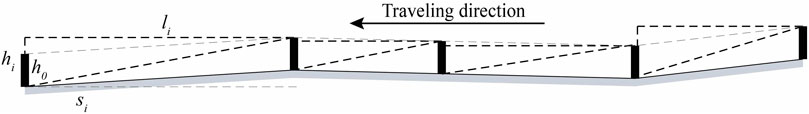
FIGURE 3. Laser rangefinder-based grade measurement method.

2.1.3.2 On-road data collection and analysis

The atmospheric pressure sensors, OBD-II Interface, GPS module, and gas analysis module were carried by the measured vehicle as it traveled along the route. The model of the tested vehicle was an Audi A4 (2.0 L, manufactured in July 2017) with cumulative mileage of 15,280 km. The second-by-second data of atmospheric pressure, temperature, GPS location, vehicle ECU data, and mass emission rates were collected. In order to ensure that the atmospheric pressure measured by the sensors can represent the ambient pressure of the vehicle, the sensors should be set outside the vehicle, or keep the windows open while the sensors were set inside the vehicle to ensure that the atmospheric pressures inside and outside the vehicle were consistent through air circulation. The road grade data were calculated by adopting the following steps.

2.1.3.2.1 Pressure-altitude relationship:

A strong relationship exists between atmospheric pressure, sea level atmospheric pressure, temperature, and altitude. Meteorological data (NMSDC, 2020) (1 January to 31 December 2019) recorded at five weather stations within Chengdu were used to modify the constants in the empirical formula (World Meteorological Organization, 2007; Keisan, 2018). The modified formula was as follows:

$H=(\frac{T}{9.4794\sqrt{\raisebox{1ex}{$p$}\!\left/ \!\raisebox{-1ex}{$p_0$}\right.}}-T)/0.0036(2)$

where p is atmospheric pressure, p₀ is sea level atmospheric pressure, H is altitude, and T is thermodynamic temperature. Based on the altitudes of the five meteorological stations within Chengdu and their published temperature and sea level atmospheric pressure data, the atmospheric pressures were calculated using Eq. 2. The coefficient of determination (R²) between the published atmospheric pressure and calculated atmospheric pressure was 0.99, and the root mean square error (RMSE) was 0.7 (Supplementary Figure S5), indicating that the formula is very accurate for the description of pressure-altitude relationship.

On the basis of the modified formula, the second-by-second altitude was then calculated using the atmospheric pressure, temperature, and sea level atmospheric pressure. The atmospheric pressure and temperature data were measured directly by the pressure sensors, and the sea level pressure data for each second were obtained by linear interpolation based on hourly data from local weather stations. Because the variation of sea level atmospheric pressure is small over short periods and is unaffected by change of elevation, the sea level atmospheric pressure data from this source had little effect on the calculation of altitude. By setting different values of T, p, and p₀, the sensitivity of the estimation of altitude to temperature, pressure, and sea level pressure was analyzed. Furthermore, the corresponding cumulative distance for the pressure-sensor-based altitude data could be calculated by summing the velocity values.

2.1.3.2.2 Fourier transform filtering:

Pressure data measured by the atmospheric pressure sensors contain noise, and therefore the calculated altitude data were filtered using the Fourier transform. To quantify the best threshold for filtering, the relative altitude data measured by the laser rangefinder were used as reference. The steps of filtering were as follows.

2.1.3.2.3 Pressure-based road grade calculation:

The filtered cumulative distance-altitude series was used to calculate the road grade series for each road section using Eq. 4:

$grad{e}_{\left(m,n\right)}=\raisebox{1ex}{$\left(altitud{e}_n-altitud{e}_m\right)$}\!\left/ \!\raisebox{-1ex}{$\left({distance}_n-{distance}_m\right)$}\right.(4)$

where m and n are the start and end points of the road section, respectively, distance_m and distance_n are the cumulative distances of location m and n on the measurement route, respectively, and altitude_m and altitude_n are the altitudes of location m and n on the measurement route, respectively. The altitude and cumulative distance for each location were obtained by interpolation using the filtered cumulative distance-altitude curve.

2.1.4 Results verification

With reference to the division of the road segment measured by the laser rangefinder and using Eq. 4, the grade of each road segment was calculated based on the altitude data measured by the atmospheric pressure sensor. Similarly, the grade data of each road segment based on GPS altitude were also calculated. Regression analysis then was performed to verify the accuracy of the grade data obtained from the different sources (i.e., BMP180, BMP3988, and GPS). The results of the regression analysis including slope, R², and RMSE were used to quantify the accuracy of each method. The regression analysis involved the linear least squares model, which is commonly used in many fields and thus further details are not repeated here.

2.2 Applications

2.2.1 VSP calculation and comparison based on different grade data

The second-by-second VSP data of the validation section were calculated separately based on road grade data obtained from the BMP180 pressure sensor, BMP388 pressure sensor, GPS, and laser rangefinder. The speed data and acceleration data of the corresponding positions were obtained from the OBD-II interface. The VSP calculation method was as follows (EPA, 2002):

$VSP=0.278\upsilon \left(0.305a+9.81\sin \left(a\cdot \tan \left(s/100\right)\right)+0.132\right)+0.0000065{\upsilon }^3(5)$

where VSP is vehicle specific power (kW/t), v is vehicle speed (km/h), a is acceleration [(km/h)/s], and s is road grade (%).

Taking VSP data based on road grade data obtained from the laser rangefinder as standard, regression analysis was performed with VSP data based on road grade data obtained from each of the other sources. The values of slope, R², and RMSE of the regression analyses were used to quantify the accuracy of the VSP data based on the different methods.

2.2.2 Calculation of emission rates for different road grades and VSP bins

On the basis of the vehicle driving cycle data and mass concentration of exhaust pollutants measured by the gas analysis module (the parameters of the gas analysis modules were introduced in the Supplementary Appendix) (InfraTec, 2020; itg, 2018, itg, 2018), the second-by-second emission rates of several pollutants (i.e., CO₂, CO, NO, and HC) were calculated for the entire route based on the mass-balance-based approach and ideal gas law, as reported in the literature (Zhang, 2006). The road grade and VSP data were divided into several bins, and the average emission rates of the pollutants corresponding to different road grade bins and VSP bins were calculated and compared.

3 Results and discussion

3.1 Altitude calculation sensitivity analysis

By setting different values of T, p, and p₀ in Eq. 2, the sensitivity of the altitude estimation to temperature, pressure, and sea level pressure was determined as 1.79 m/°C, −9.06 m/hPa, and 8.53 m/hPa, respectively. In this study, both temperature and pressure were measured with accuracy of 0.5°C and 0.08 hPa (relative accuracy), respectively, and therefore all the errors were <1 m. The pressure at sea level data were released by the national meteorological stations. Sea level pressure changes little over short periods and its hourly variation is generally not greater than 0.4 hPa; that is, the cumulative error of the distance measurement in an hour is <5 m. Thus, the altitude results calculated using this method satisfy the research requirements.

3.2 Comparison of altitude and grade acquisition of different devices

The on-road measurements were conducted twice in the morning and afternoon of the 14th January, a cloudy day. In the morning measurement, the sea-level pressure was 1,016.91 ± 0.36 hPa and the temperature was 8.6 ± 0.26°C. In the afternoon measurement, the sea-level pressure was 1,012.76 ± 0.33 hPa and the temperature was 5.6 ± 0.25°C (according to the integrated hourly data recorded at the national meteorological station on the same day). The results of morning measurement were mainly analyzed in the manuscript, the results of afternoon measurement were shown in the Supplementary Appendix.

The time-pressure curve and cumulative distance-altitude curve based on the two types of atmospheric pressure sensor are shown in Figures 4A, B, respectively. The two sets of pressure series and altitude series (after filtering) are consistent, which shows that the pressure sensors reflect the real pressure variation precisely, and that filtering can eliminate the influence of sensor noise and better reflect the actual elevation. The altitude series both show a trend of initial decrease followed by increase, which is consistent with the terrain of Chengdu. Additionally, the elevation changes associated with overpasses and underpass tunnels (Figure 2 and Figure 4B) are obvious.

FIGURE 4

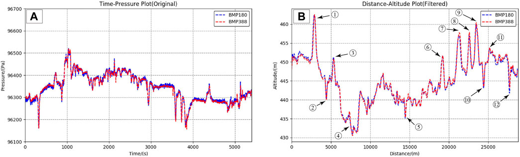
FIGURE 4. Comparison of pressure variation (A) and altitude variation (B) over entire on-road measurement route based on two types of pressure sensor.

The relative altitude and grade variations for the validation section of the measurement route based on different data sources are shown in Figures 5A, B, respectively. Taking the curves based on the laser rangefinder as reference, the altitude variation and grade variation based on the pressure sensors (BMP180 and BMP388) are much more precise than the GPS results. In particular, the altitude and grade variations associated with overpasses and underpass tunnels are obvious.

FIGURE 5

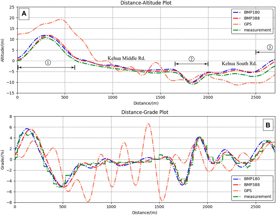
FIGURE 5. Altitude (A) and grade (B) variations of validation section based on different methods.

Using the laser rangefinder results as reference, the absolute deviation and relative deviation of the slope measurement results of each road section based on the different methods are shown in Supplementary Table S1, and the average values are shown in Table 3.

TABLE 3

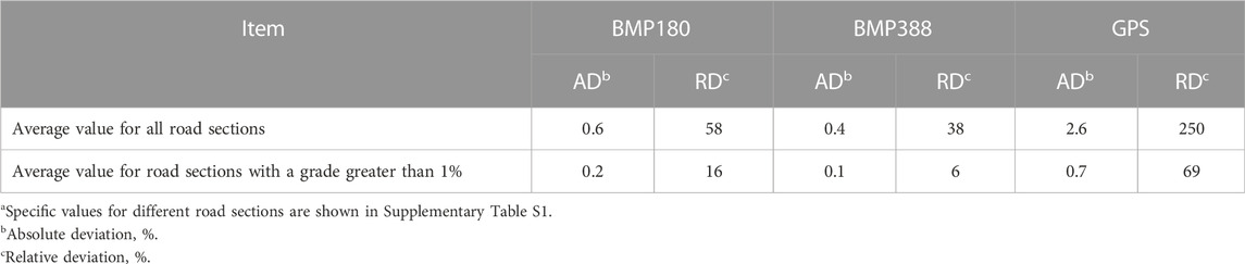
TABLE 3. Comparison of average grade data of measurement road sections obtained using different methods^a.

The accuracy of the BMP388 measurement results is best, that is, the average absolute deviation for all road sections is 0.4%, and the average absolute (relative) deviation for road sections with slope >1% is only 0.1% (6%). The accuracy of the BMP180 results is slightly lower than that of the BMP388 results, and the accuracy of the GPS results is poorest.

The regression results between the laser rangefinder grade data and other road grade data are shown in Figure 6. The grade data based on the BMP388 pressure sensor have the strongest correlation with the laser rangefinder grade data, with values of R², RMSE, and slope of 0.94, 0.45%, and 1.0, respectively, meaning that the accuracy and precision of the BMP388 results are best. The values of R², RMSE, and slope of the BMP180 results are 0.91, 0.45%, and 1.0, respectively, meaning that the measurement results based on the BMP180 sensor are also relatively satisfactory. The regression results for the GPS-based grade data are poorest, with values of R², RMSE, and slope of 0.11, 2.58% and 0.4, respectively.

FIGURE 6

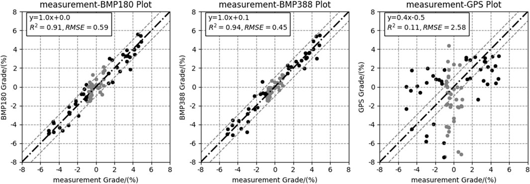
FIGURE 6. Scatter plots between grade based on real-world measured grade data (laser rangefinder) and grade data based on BMP180 pressure sensor, BMP388 pressure sensor, and GPS data.

3.3 Comparison of VSP results based on different road grade data

On the basis of grade data obtained using the different methods, the VSP variations for the validation section of the measurement route were calculated (Figure 7). The variations of VSP data based on the BMP388 and BMP180 sensors are consistent with the laser rangefinder-based VSP data; the performance of the former sensor is most consistent with the laser rangefinder-based VSP data. It can be seen that the VSP data based on the GPS method do differ from the laser rangefinder-based VSP data; for many road sections, the VSP values and variation trends of the two methods are markedly different.

FIGURE 7

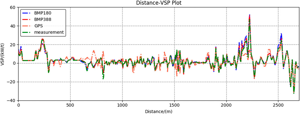
FIGURE 7. VSP variations of validation section based on different methods.

The regression results between the laser rangefinder-based VSP data and that of the other methods are shown in Figure 8. The calculated VSP based on the BMP388 pressure sensor grade data has the strongest correlation with that determined using the laser rangefinder-based grade data, with values of R², RMSE, and slope of 0.99, 0.25 kW/t, and 1.0, respectively, meaning that the accuracy and precision of the BMP388 results are best. The regression results of the GPS-based VSP data are poorest, with values of R², RMSE, and slope of only 0.46, 1.71 kW/t, and 0.6, respectively. The results of afternoon measurement also showed a strong correlation between pressure-based data and laser rangefinder-based data (Supplementary Figures S4, S5). The results of both independent measurements were good, confirming to some extent the accuracy of the framework.

FIGURE 8

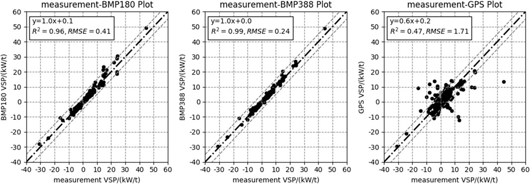
FIGURE 8. Scatter plots between VSP based on real-world measured grade data (laser rangefinder) and VSP data based on BMP180 pressure sensor, BMP388 pressure sensor, and GPS data.

3.4 Emission rates for different road grade bins and VSP bins

The emission rates of pollutants for different grade bins are shown in Figure 9. Generally, with an increase of road grade, the average emission rates of pollutants increase obviously. On flat road sections and road sections with small negative grade, the emission rates are similar. The emission rates on road sections with positive grade are obviously higher, whereas the emission rates on road sections with higher negative grade are obviously lower. The emission rates for road grade of >3% can be three to six times greater than the emission rates for road grade of <−3%. Overall, NO_x has the largest relative change in emission rate. The changes in CO₂ emission rate are highly correlated with fuel consumption rate. Because the vehicle experiences greater power demand on positively graded roads, there is greater fuel use and corresponding increase of CO₂ emissions.*Grade bin:1: (−∞, −3%); 2: (−3%, −0.5%); 3: (−0.5%, 0.5%); 4: (0.5%, 3%); 5: (3%, +∞).

FIGURE 9

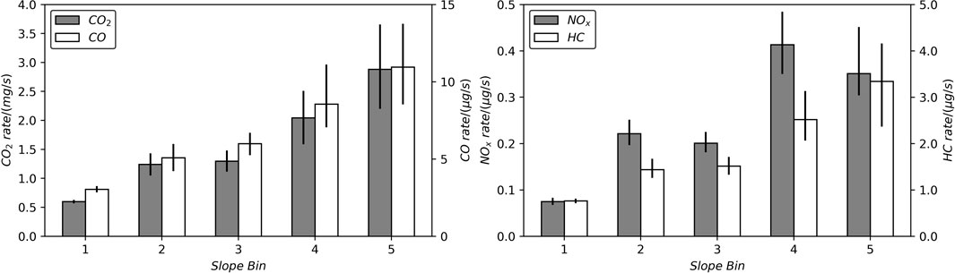
FIGURE 9. Pollutant emission rates for different grade bins.

A comparison of on-road measurements in different research were conducted, and the average emission rates based on the definition of road grade bins in this study were calculated. Due to the differences in vehicle types among studies, the ratios of emission rates were calculated for different grade bins using the emission rates of flat roads (Bin 3 in this study) as a baseline (Table 4).

TABLE 4

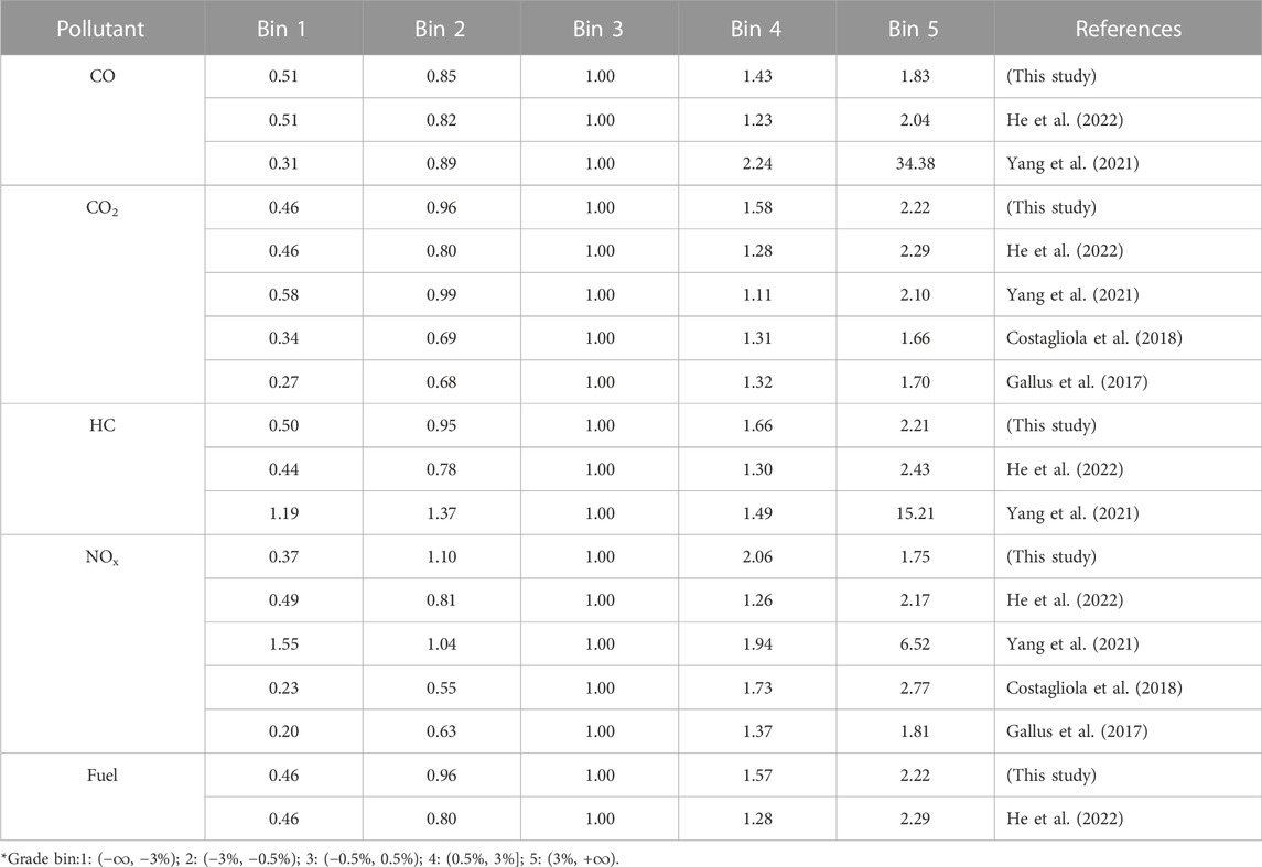
TABLE 4. Comparison of pollutant average emission rate ratios in different research using flat road (Bin 3 in this study) emission rates as a baseline.

As shown in Table 4, the general trend of increasing emission rates of most pollutants with increasing road grade was consistent. For example, the average emission rates of several pollutants for grade bin 2 were generally 0.7–0.9 of that for flat road, and the average emission rates for grade bin 1 were about 0.5 or less of that for flat road. For uphill road sections, the average emission rates for grade bin 4 were 1.2–1.8 of that of flat road, and the average emission rates for grade bin 5 were 2 or more of that of flat road.

For NO_x, the variation characteristics of emission rates in the downhill road sections varied among studies. In this study and in Yang’s study (2021), the average emission rates of NO_x appeared increase in downhill road sections. The reason for this may be the different driving habits of drivers. For example, some drivers will take active brakes on downhill road sections, resulting in variation in engine operating conditions. Due to the delay in the adjustment of air-fuel ratio in some vehicles, excessive air intake will lead to an increase in NO_x emissions. However, it is worth doing more further analysis to confirm whether this is a general characteristic.

The emission rates of pollutants for different VSP bins are shown in Figure 10. It can be seen that an increase of VSP leads to obvious increase in the average emission rates of pollutants. The mean emission rates of several pollutants are lowest for mode 3, which includes idling, and they increase monotonically with VSP mode as VSP increases. The average emission rates for negative VSP, which includes deceleration, are higher than for idling but less than for values of positive VSP. The use of road grade information for estimation of emissions is not limited to the VSP-based approach illustrated here. Road grade can be used as an explanatory variable in other modeling frameworks.^*VSP bin:1: (−∞, −5); 2: (−5, 0); 3: (0, 1); 4: (1, 5); 5: (5, 10); 6: (10, 20); 7: (20, 30); 8: (30, +∞).

FIGURE 10

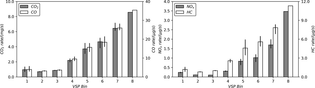
FIGURE 10. Pollutant emission rates for different VSP bins.

4 Conclusion

This study developed a framework for road grade measurement based on an electronic atmospheric pressure sensor. Although noise in the sensor measurements might affect the results, this drawback can be overcome by filtering. Additionally, the altitude calculation based on atmospheric pressure might also affect the accuracy of results; however, the sensitivity analysis results indicated that such impact is limited.

Verification of the measurement results showed that grade data calculated based on an electronic atmospheric pressure sensor can accurately reflect reality. The emission rates of pollutants calculated based on the derived grade data were found to be sensitive to grade variation and VSP variation; increases of grade and VSP led to obvious increase in average emission rates of pollutants. The findings illustrate that atmospheric pressure sensor data can be sufficiently reliable and accurate for road grade measurement for on-road vehicle emissions modeling.

Of course, this framework has the need for further research. For example, more tests under different seasons and weather conditions need to be conducted to verify the influence of different factors on the applicability of the method.

Data availability statement

The original contributions presented in the study are included in the article/Supplementary Material, further inquiries can be directed to the corresponding author.

Author contributions

Equipment integration: XM, KP, and WL; Experimental design: XM, BD, and YW; Experimental execution: XM, KP, JZ, and YX; Data processing and graphing: XM and KP; Article writing: XM; Article check and revision: BD and KP.

Funding

This study is supported by the National Natural Science Foundation of China (grant number 41877395). Any opinions, findings, and conclusion or recommendations expressed in this material are those of the author(s) and do not necessarily reflect the views of the Natural Science Foundation Committee of China and the Ministry of Environmental Protection of PRC.

Conflict of interest

The authors declare that the research was conducted in the absence of any commercial or financial relationships that could be construed as a potential conflict of interest.

Publisher’s note

All claims expressed in this article are solely those of the authors and do not necessarily represent those of their affiliated organizations, or those of the publisher, the editors and the reviewers. Any product that may be evaluated in this article, or claim that may be made by its manufacturer, is not guaranteed or endorsed by the publisher.

Supplementary material

The Supplementary Material for this article can be found online at: https://www.frontiersin.org/articles/10.3389/fenvs.2022.1051858/full#supplementary-material

References

Arduino, U. (2020). Rev3. Available at: https://store.arduino.cc/usa/arduino-uno-rev3.

Google Scholar

Awuah-Baffour, R., Sarasua, W., Dixon, K. K., Bachman, W., and Guensler, R. (1997). Global positioning system with an attitude: Method for collecting roadway grade and superelevation data. Transp. Res. Rec. 1592, 144–150. doi:10.3141/1592-17

CrossRef Full Text | Google Scholar

Bae, H. S., Ryu, J., and Gerdes, C. (2001). “Road grade and vehicle parameter estimation for longitudinal control using GPS,” in Presented at the IEEE conference on intelligent transportation systems (Alameda, CA: Intelligent Transportation Systems Society).

Google Scholar

Bindschadler, R., Fahnestock, M., and Sigmund, A. (1999). Comparison of Greenland ice sheet topography measured by TOPSAR and airborne laser altimetry. IEEE Trans. Geosci. Remote Sens. 237, 2530–2535. doi:10.1109/36.789648

CrossRef Full Text | Google Scholar

BOSCH (2015). BMP180 Digital pressure sensor Restricted data sheet. Available at: https://www.mouser.com/datasheet/2/783/BST-BMP180-DS000-1509579.pdf.

Google Scholar

BOSCH (2018). BMP388 Digital pressure sensor Restricted data sheet. Available at: https://ae-bst.resource.bosch.com/media/_tech/media/datasheets/BST-BMP388-DS001.pdf.

Google Scholar

Chong, H., Kwon, S., Lim, Y., and Lee, J. (2020). Real-world fuel consumption, gaseous pollutants, and CO2 emission of light-duty diesel vehicles. Sustain. Cities Soc. 53, 101925. doi:10.1016/j.scs.2019.101925

CrossRef Full Text | Google Scholar

Cicero-Fernandez, P., Long, J. R., and Winer, A. M. (1997). Effects of grades and other loads on on-road emissions of hydrocarbons and carbon monoxide. J. Air Waste Manag. Assoc. 47, 898–904. doi:10.1080/10473289.1997.10464455

PubMed Abstract | CrossRef Full Text | Google Scholar

Costagliola, M. A., Costabile, M., and Prati, M. V. (2018). Impact of road grade on real driving emissions from two Euro 5 diesel vehicles. Appl. Energy 231, 58C6–593. doi:10.1016/j.apenergy.2018.09.108

CrossRef Full Text | Google Scholar

Denis, M. J., Cicero-Fernandez, P., Winer, A. M., Butler, J. W., and Jesion, G. (1994). Effects of in-use driving conditions and vehicle/engine operating parameters on off- cycle events: Comparison with federal test procedure conditions. Air Waste 44, 31–38. doi:10.1080/1073161x.1994.10467235

CrossRef Full Text | Google Scholar

Denis, M. J., and Winer, A. M. (1993). “Prediction of on-road emissions and comparison of modeled on-road emissions to federal test procedure emissions,” in Presented at the specialty conference on the emission inventory: Perception and reality of A&WMA (Pittsburgh, PA: Air & Waste Management Association).

Google Scholar

ELM Electronics (2020). Obd. Available at: https://www.elmelectronics.com/products/ics/obd/.

Google Scholar

Enns, P., German, J., and Markey, J. (1993). “US EPA’s survey of in-use driving patterns: Implications for mobile source emission inventories,” in Presented at the specialty conference on the emission inventory: Perception and reality of A&WMA (Pittsburgh, PA: Air & Waste Management Association), 914.

Google Scholar

EPA (2002). EPA’s onboard analysis shootout: Overview and result; epa420-R-02– 026; office of transportation and air quality. Ann Arbor, MI: U.S. Environmental Protection Agency.

Google Scholar

Frey, H. C., Unal, A., Chen, J., Li, S., and Xuan, C. (2002). “Methodology for developing modal emission rates for EPA’s multi-scale motor vehicle & equipment emission system; epa420-R-02-02,” in Prepared by North Carolina state university for office of transportation and air quality (Ann Arbor, MI: U.S. Environmental Protection Agency).

Google Scholar

Gallus, J., Kirchner, U., Vogt, R., and Benter, T. (2017). Impact of driving style and road grade on gaseous exhaust emissions of passenger vehicles measured by a Portable Emission Measurement System (PEMS). Transp. Res. Part D Transp. Environ. 52, 215–226. doi:10.1016/j.trd.2017.03.011

CrossRef Full Text | Google Scholar

He, L., You, Y., Zheng, X., Zhang, S., Li, Z., Zhang, Z., et al. (2022). The impacts from cold start and road grade on real-world emissions and fuel consumption of gasoline, diesel and hybrid-electric light-duty passenger vehicles. Sci. Total Environ. 851, 158045. doi:10.1016/j.scitotenv.2022.158045

PubMed Abstract | CrossRef Full Text | Google Scholar

Hernandez-Pajares, M., Zomoza, J. M. J., Subirana, J. S., and Colombo, O. L. (2003). Feasibility of wide-area subdecimeter navigation with GALILEO and modernized GPS. IEEE Trans. Geosci. Remote Sens. 241, 2128–2131. doi:10.1109/tgrs.2003.817209

CrossRef Full Text | Google Scholar

Hill, J. M., Graham, L. A., and Henry, R. J. (2000). Wide-area topographic mapping and applications using airborne light detection and ranging (LiDAR) technology. Photogram. Eng. Remote Sens. 66, 908–914.

Google Scholar

InfraTec (2020). Multi-channel pyroelectric detector. Available at: https://www.infratec-infrared.com/downloads/en/sensor-division/detector_data_sheet/infratec-datasheet-lrm-244-_.pdf.

Google Scholar

itg (2018). Product Specification of: NO-Automotive Sensor/Type A-22. Available at: http://www.it-wismar.de//_documents/specs/A-22_spec.pdf.

Google Scholar

itg (2012). Product Specification of: O2-Industrial Sensor/Type I-01. Available at: http://www.itg-wismar.de/_documents/specs/I-01_spec.pdf.

Google Scholar

Jimenez-Palacios, J. L. (1999). Massachusetts institute of technology. Ph.D. Thesis. Cambridge, MA: Dept. of Mechanical Engineering.

Google Scholar

Keisan (2018). Convert pressure. Available at: https://keisan.casio.jp/keisan/image/Convertpressure.pdf.

Google Scholar

Kelly, N., and Groblicki, P. J. (1993). Real-world emissions from a modern production vehicle driven in los angeles. Air Waste 43, 1351–1357. doi:10.1080/1073161x.1993.10467209

CrossRef Full Text | Google Scholar

LaserTec (2020). Trupulse200 specifications. Available at: https://www.lasertech.com/TruPulse-200-Rangefinder.aspx itg.

Google Scholar

Lefsky, M. A., Cohen, W. B., Parker, G. G., and Harding, D. J. (2002). LiDAR: Remote sensing for ecosystem studies. Bioscience 52, 19–30. doi:10.1641/0006-3568(2002)052[0019:lrsfes]2.0.co;2

CrossRef Full Text | Google Scholar

Lim, K., Treitz, P., Wulder, M., St-Onge, B., and Flood, M. (2003). LiDAR: Remote sensing of forest structure. Prog. Phys. Geogr. Earth Environ. 27, 88–106. doi:10.1191/0309133303pp360ra

CrossRef Full Text | Google Scholar

Liu, H., Rodgers, M., and Guensler, R. (2019). Impact of road grade on vehicle speed-acceleration distribution, emissions and dispersion modeling on freeways. Transp. Res. Part D Transp. Environ. 69, 107–122. doi:10.1016/j.trd.2019.01.028

CrossRef Full Text | Google Scholar

Nam, E. K. (2003). “Proof of concept investigation for the physical emissions estimator (PERE) for MOVES; epa420-R-03-00,” in Prepared by ford Re- search and advanced engineering for assessment and standards division, office of transportation and air quality (Ann Arbor, MI: U.S. Environmental Protection Agency).

Google Scholar

NMSDC (National Meteorological Science Data Center) (2020). National meteorological science data center. Available at: http://data.cma.cn/site/index.html.

Google Scholar

North Carolina Floodplain Mapping Program (2013). LiDAR and digital elevation data. Available at: http://www.ncfloodmaps.com/pubdocs/lidar_final_jan03.pdf.

Google Scholar

Perugu, H. (2019). Emission modelling of light-duty vehicles in India using the revamped VSP-based MOVES model: The case study of Hyderabad. Transp. Res. Part D Transp. Environ. 68, 150–163. doi:10.1016/j.trd.2018.01.031

CrossRef Full Text | Google Scholar

Pierson, W. R., Gertler, A. W., Robinson, N. F., Sagebiel, J. C., Zielinska, B., Bishop, G. A., et al. (1996). Real-world automotive emissions: Summary of studies in the fort McHenry and tuscarora mountain tunnels; atmos. Atmos. Environ. X. 30, 2233–2256. doi:10.1016/1352-2310(95)00276-6

CrossRef Full Text | Google Scholar

Rosero, F., Fonseca, N., López, J., and Casanova, J. (2021). Effects of passenger load, road grade, and congestion level on real-world fuel consumption and emissions from compressed natural gas and diesel urban buses. Appl. Energy 282, 116195. doi:10.1016/j.apenergy.2020.116195

CrossRef Full Text | Google Scholar

SciPy community (2020). Discrete fourier transform. Available at: https://docs.scipy.org/doc/numpy/reference/generated/numpy.fft.fft.html#numpy.fft.fft.

Google Scholar

Souleyrette, R., Hallmark, S., Pattnaik, S., O’Brien, M., and Veneziano, D. (2003). “Grade and cross slope estimation from LiDAR based surface model; MTC-2001-02,” in Prepared by midwest transportation consortium and Iowa state university for U.S. Department of transportation, research and special programs administration (Washington, DC: U.S. Department of Transportation).

Google Scholar

Sun, G., and Ranson, K. J. (2000). Modeling LiDAR returns from forest canopies. IEEE Trans. Geosci. Remote Sens. 38, 2617–2626. doi:10.1109/36.885208

CrossRef Full Text | Google Scholar

Toutin, T. (2004). Comparison of stereo-extracted DTM from different high- resolution sensors: SPOT-5, EROS-a, IKONOS-II, and QuickBird. IEEE Trans. Geosci. Remote Sens. 42, 2121–2129. doi:10.1109/tgrs.2004.834641

CrossRef Full Text | Google Scholar

Wanninger, L. (2018). Introduction to network RTK. IAG Work. Group 4, 5–1. Avaliable at: www.wasoft.de.

Google Scholar

World Meteorological Organization (2007). CIMO/ET-Stand-1/Doc.10(20.XI.2012). Available at: https://www.wmo.int/pages/prog/www/IMOP/meetings/SI/ET-Stand-1/Doc-10_Pressure-red.pdf.

Google Scholar

Yang, H. H., Dhital, N. B., Cheruiyot, N. K., Wang, L. C., and Wang, S. X. (2021). Effects of road grade on real-world tailpipe emissions of regulated gaseous pollutants and volatile organic compounds for a Euro 5 motorcycle. Atmos. Pollut. Res. 12 (9), 101167. doi:10.1016/j.apr.2021.101167

CrossRef Full Text | Google Scholar

Yazdani Boroujeni, B., and Frey, H. (2014). Road grade quantification based on global positioning system data obtained from real-world vehicle fuel use and emissions measurements. Atmos. Environ. X. 85, 179–186. doi:10.1016/j.atmosenv.2013.12.025

CrossRef Full Text | Google Scholar

Zhang, K., Chen, S., Whitman, D., Shyu, M., Yan, J., and Zhang, C. A. (2003). A progressive morphological filter for removing nonground measurements from airborne LIDAR data. IEEE Trans. Geosci. Remote Sens. 141, 872–882. doi:10.1109/tgrs.2003.810682

CrossRef Full Text | Google Scholar

Zhang, K., and Frey, H. C. (2012). Road grade estimation for on-road vehicle emissions modeling using light detection and ranging data. J. Air Waste Manag. Assoc. 56, 777–788. doi:10.1080/10473289.2006.10464500

PubMed Abstract | CrossRef Full Text | Google Scholar

Zhang, K. (2006). Micro-scale on-road vehicle-specific emissions measurements and modeling. PhD dissertation. Raleigh, NC: North Carolina State University.

Google Scholar

Zhang, L., Hu, X., Qiu, R., and Lin, J. (2019). Comparison of real-world emissions of LDGVs of different vehicle emission standards on both mountainous and level roads in China. Transp. Res. Part D Transp. Environ. 69, 24–39. doi:10.1016/j.trd.2019.01.020

CrossRef Full Text | Google Scholar

Zhang, L., Lin, J., and Qiu, R. (2021). Characterizing the toxic gaseous emissions of gasoline and diesel vehicles based on a real-world on-road investigation. J. Clean. Prod. 286, 124957. doi:10.1016/j.jclepro.2020.124957

CrossRef Full Text | Google Scholar