 Lei Yan
 Qingwen Lei1,2
 Cong Jiang
94% of researchers rate our articles as excellent or good
Learn more about the work of our research integrity team to safeguard the quality of each article we publish.
Find out more
ORIGINAL RESEARCH article
Front. Environ. Sci., 17 November 2022
Sec. Atmosphere and Climate
Volume 10 - 2022 | https://doi.org/10.3389/fenvs.2022.1049840
This article is part of the Research TopicHydro-Climate Extremes and Natural Disasters During Global Warming: Observation, Projection, and MitigationView all 11 articles
Accurate runoff prediction can provide a reliable decision-making basis for flood and drought disaster prevention and scientific allocation of water resources. Selecting appropriate predictors is an effective way to improve the accuracy of runoff prediction. However, the runoff process is influenced by numerous local and global hydrometeorological factors, and there is still no universal approach about the selection of suitable predictors from these factors. To address this problem, we proposed a runoff prediction model by combining machine learning (ML) and feature importance analysis (FIA-ML). Specifically, take the monthly runoff prediction of Yingluoxia, China as an example, the FIA-ML model uses mutual information (MI) and feature importance ranking method based on random forest (RF) to screen suitable predictors, from 130 global climate factors and several local hydrometeorological information, as the input of ML models, namely the hybrid kernel support vector machine (HKSVM), extreme learning machine (ELM), generalized regression neural network (GRNN), and multiple linear regression (MLR). An improved particle swarm optimization (IPSO) is used to estimate model parameters of ML. The results indicated that the performance of the FIA-ML is better than widely-used long short-term memory neural network (LSTM) and seasonal autoregressive integrated moving average (SARIMA). Particularly, the Nash-Sutcliffe Efficiency coefficients of the FIA-ML models with HKSVM and ELM were both greater than 0.9. More importantly, the FIA-ML models can explicitly explain which physical factors have significant impacts on runoff, thus strengthening the physical meaning of the runoff prediction model.
Water resources are important for social and economic development and the ecological environment, and accurate runoff forecasting can provide a reasonable decision-making basis for the optimal allocation and utilization of water resources (Huang et al., 2014; Xiong et al., 2019; Feng et al., 2020a; Yan et al., 2021a; Jian et al., 2022). However, under changing environments, the runoff process and associated hydrological system have been altered by human activities and climate change (Song et al., 2018; Sun et al., 2018, 2022; Jiang et al., 2019; Lu et al., 2020; Yan et al., 2020; Hu et al., 2022), and the runoff series becomes nonlinear and nonstationary, which makes it challenging to capture the variation characteristics of runoff (Sun et al., 2014; Lin et al., 2020; Yan et al., 2021b; Samantaray et al., 2022a; Samantaray et al., 2022b; Samantaray et al., 2022c; Zhou et al., 2022). Therefore, there is an urgent need to develop a runoff prediction model with robustness and high forecasting accuracy under a changing environment (Sit et al., 2020; Niu et al., 2021; Zhao et al., 2021). In recent years, there have been many studies trying to transform the complex runoff series into stationary sub-sequences using wavelets or mode decomposition methods, and then predict the sub-sequences to improve the accuracy of prediction (Meng et al., 2019; Feng et al., 2020b; Niu et al., 2020). However, these studies often ignore the relationship between hydrometeorological factors and the variation characteristics of runoff.
As revealed by recent studies, the changing characteristics of runoff process are controlled by numerous factors, such as astronomy, meteorology, ocean, and underlying surface conditions (Tang et al., 2018; Shi et al., 2021; Bian et al., 2022; Ma et al., 2022). When there are no significant changes for the underlying surface conditions, the runoff process mainly depends on precipitation and evaporation, which are influenced by atmospheric circulations (Talaee et al., 2014; Huang et al., 2017; Luo et al., 2017). On the other hand, the interaction between the ocean and the atmosphere drives the exchange of matter and energy between regions of the Earth, which can affect regional weather and climate change (Nugent and Matthews, 2012; Singh and Roxy, 2022). Therefore, the sea temperature indices, such as Pacific Decadal Oscillation Index (PDO) and El Niño–Southern Oscillation index (ENSO), are also important affecting factors of runoff (Yang et al., 2021; You et al., 2021). From the analysis of the physical mechanism of runoff, atmospheric circulation, sea temperature index, precipitation, and evaporation are all important influencing factors in the runoff prediction.
Variations of runoff are closely related to large-scale climate factors in hydrometeorological teleconnection analysis (Lima and Lall, 2010; Peters et al., 2013; Steinschneider and Lall, 2016; Wang et al., 2022). Therefore, many studies combining teleconnection analysis have been proposed to strengthen the physical meaning of runoff prediction. Wang et al. (2020) established a runoff prediction model by combining teleconnection analysis and ensemble empirical mode decomposition (EEMD) and achieved good application results, but they mentioned the cross-correlation method used in their paper is not suitable for analyzing nonlinearity and non-stationary time series. Maity and Kashid (2011) combined genetic programming (GP) with importance analysis, and used global climate factors and local meteorological variables as predictors to carry out the weekly-scale runoff forecasting for the Mahanadi River in India. It has been proved that the model derived by GP for a complex runoff system can effectively improve the accuracy of weekly runoff prediction. Yang et al. (2017) selected 17 known climate phenomenon indices, such as PDO and ENSO, and used several machine learning (ML) regression models to predict and simulate the runoff 1-month in advance of headwater reservoirs in USA and China. The results indicated that the climate phenomenon indices are beneficial for improving the accuracy of monthly or seasonal reservoir runoff prediction.
Based on the previous studies, we can find that enriching the input features of regression models is an effective method to improve the accuracy of runoff prediction. However, since numerous physical factors are expected to jointly affect the variation of runoff, there is expected to exist a mutual correlation among these factors. Thus, finding a suitable set of predictors from the high-dimensional data, consist of physical factors, as the input of the runoff prediction model is still a challenge for medium and long-term runoff prediction. In information theory, mutual information (MI) method is a powerful tool for analyzing linear and nonlinear relationships between variables (Elkiran et al., 2021), but simply selecting predictors through correlation analysis provided by MI will introduce many redundant features (Tiwari and Chaturvedi 2022). To solve this problem, in traditional high-dimensional data preprocessing, principal component analysis (PCA) is typically used to reduce dimensionality and it can effectively reduce redundant variables and feature dimensions (Ouyang et al., 2022). But PCA cannot accurately measure the importance of each feature on runoff prediction results. Thus, how to select the input predictors of regression model needs further investigation. In this study, we attempted to develop a runoff prediction model by combining ML with importance analysis for each feature (FIA-ML) to improve the accuracy of runoff prediction and explain the variation law of runoff from the view of physical causes.
In a summary, the aims of this study are: 1) to select appropriate predictors according to the importance measures computed by random forest (RF) for each feature; and 2) to construct the runoff prediction models by fitting the correlation between predictors and monthly runoff based on the ML models, whose hyper-parameters are optimized by an improved particle swarm optimization (IPSO). To fulfill these aims, the monthly runoff data collected from the Yingluoxia station in China was selected for illustration purposes, and the performance of the developed FIA-ML models was compared with two widely-used runoff time series analysis models, i.e., long short-term memory neural network (LSTM) and seasonal autoregressive integrated moving average (SARIMA).
The Heihe River Basin (HRB) is the second-largest inland watershed in Northwest China, whose geographic coordinates are roughly between
The HRB originates from the Qilian Mountains in the south, with a total length of 821 km. It flows through Qinghai, Gansu, and Inner Mongolia provinces and finally into Juyanhai. In this study, the Yingluoxia basin (YLX) is selected as the study area, which is in the upper reaches of the HRB, with a controlled catchment area of about
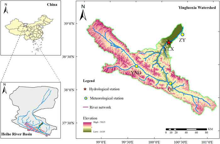
FIGURE 1. The location of the study area and meteorological observation stations. YNG denotes Yeniugou (Meteorological station 1), ZY denotes Zhangye (Meteorological station 2), QL denotes Qilian (Meteorological station 3) and YLX denotes Yingluoxia (Hydrological station).
The 130 large-scale climate factors used in this study are provided by the National Climate Center of China Meteorological Administration (NCC-CMA) (https://cmdp.ncc-cma.net/cn/download.htm), including 88 atmospheric circulation indices, 26 sea temperature indices, and 16 other indices. In this study, these large-scale climate factors are sequentially numbered for 1–130, which is consistent with the serial number of the datasets provided by the NCC-CMA. As for the local meteorological information, namely the evaporation (factor numbers: 131–133) and precipitation data (factor numbers: 134–136) of the Yeniugou (YNG), Zhangye (ZY), and Qilian (QL) meteorological stations, are collected from the National Tibetan Plateau/Third Pole Environment Data Center (https://data.tpdc.ac.cn/zh-hans/). In addition, we also considered the previous runoff of YLX (factor number: 137) as a factor. Therefore, a total of 137 physical factors were considered for further building the monthly runoff prediction model in this study.
Mutual information (MI) is a nonparametric statistical method used to measure the degree of correlation between variables. MI does not have any special requirements for the distribution type of variables, and it can describe both linear and nonlinear correlation. Therefore, it has been widely used in variable selection in hydrology, meteorology, and other fields (He et al., 2015; Fang et al., 2018). Given variables
where
MI has difficulties in estimating probability density. Thus, Kraskov et al. (2004) proposed a method based on k-nearest neighbors to avoid directly estimating the probability density of the variables. As for the significance test of MI, the method proposed by Sharma (2000) is applied, and the significance level is set to be 0.01 in this study.
Random forest (RF) is an extended variant of the bagging parallel ensemble learning method (Breiman, 2001). During the training period, it uses bootstrap sampling to generate a subset of training samples. Therefore, each base learner only uses about 63.2% of the samples in the initial training set, and the remaining 36.8% of the samples can be used as the validation set to evaluate the generalizability of RF. This way of assessing the generalization of the model is called out-of-bag (OOB) estimation.
As shown in many studies, reasonable predictors can significantly improve the accuracy and robustness of the regression model in runoff prediction (Taormina and Chau, 2015; Sharifi et al., 2017). RF can efficiently deal with the multivariate samples and measure the importance of each variable (Genuer et al., 2010; Hapfelmeier et al., 2014). The importance measure of each feature in runoff forecasting is computed as follows: 1) to obtain the mean square error vector
where
If the feature is shuffled, the greater the accuracy of OOB estimation decreases, the greater the degree of disturbance to the model by the feature. By normalizing
Support vector machines (SVM) can solve nonlinear problems, mainly using the kernel function to map the input factors to the high-dimensional space and then performing linear regression. Different kernel functions will significantly affect the fitting ability of SVM to different kinds of nonlinear problems. Among the commonly used kernel functions, the polynomial kernel function
where
Extreme learning machine (ELM) is a machine learning method based on feedforward neural network. ELM consists of a three-layer structure: input layer, hidden layer, and output layer. During the training period, the weights of the output layer can be obtained by the least square method (LSM). Given the input predictors
where
Generalized Regression Neural Network (GRNN) is of high fault tolerance and strong robustness, which is suitable for solving nonlinear problems and can also handle unstable data. The network structure of GRNN consists of the input layer, mode layer, summation layer and output layer. After the input predictors
where
Multiple Linear Regression (MLR) can be used to fit a linear relationship between multiple independent and dependent variables. After the specific MLR equation is obtained through training, the dependent variable can be predicted by the following equation:
where
The performance of machine learning (ML) may be limited in practice since its forecasting results are largely influenced by the choice of hyper-parameters. Therefore, it is critical to obtain the hyper-parameters combination with the best generalization performance. In this study, we use the K-Fold cross-validation method (Soper, 2021) to evaluate the model performance. However, the cross-validation results of ML models are sensitive to the choice of hyper-parameters. When using conventional particle swarm optimization algorithms to estimate their hyper-parameters, there are problems of premature maturity and local convergence. To overcome these problems, we employed an improved particle swarm optimization algorithm (IPSO) in this study to determine a set of hyper-parameters that optimize the cross-validation results. Please refer to Lei et al. (2022) for more details about IPSO. The hyper-parameters that need to be tuned by IPSO are displayed in Table 1.
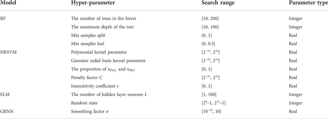
TABLE 1. The range of hyper-parameters to be optimized for the model used in this paper.
In this study, we selected several indicators to quantitatively analyze the performance of various models, which are Nash-Sutcliffe efficiency (NSE), root mean square error (RMSE), the coefficient of correlation (R), and Kling-Gupta efficiency (KGE) (Gupta et al., 2009).
The value range of
where
The smaller the RMSE, the higher the prediction accuracy. It is calculated by the following equation:
where
where
The main purpose of this study is to screen out suitable input predictors for the ML models and to explore which physical factors have a significant impact on the monthly runoff of YLX station. In this study, the monthly runoff of the first 564 months (1960–2006) of YLX station was used as training data to train the model, and the monthly runoff of the last 120 months (2007–2016) was used as testing data to test the predictive accuracy of the monthly runoff prediction model. The flowchart of the monthly runoff prediction model by combining ML with feature importance analysis (FIA-ML) is presented in Figure 2.
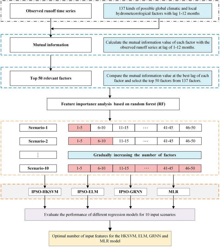
FIGURE 2. The flowchart of monthly runoff prediction using the FIA-ML model.
This study proposed a novel monthly runoff prediction model combining ML with teleconnection analysis, which is different from the commonly used time series analysis model (TSAM). Therefore, to show the superiority of the proposed FIA-ML model, it is necessary to make a comparison with some traditional TSAMs. In the following analysis, we compared the FIA-ML model with the widely used long short-term memory neural network (LSTM) and seasonal autoregressive integrated moving average (SARIMA) in previous studies. LSTM is a variant of recurrent neural network (RNN), which can effectively solve the gradient explosion or disappearance of simple RNN, and control the transfer of runoff time series information through a gating mechanism (Yuan et al., 2018; Ghose et al., 2022). Considering that the monthly runoff series is affected by the interaction of seasonal effects, long-term trend effects and random fluctuations, SARIMA transforms the nonstationary monthly runoff series into stationary series by performing trend difference and seasonal difference operation, and then establish a statistical analysis model (Valipour, 2015). The TSAM requires less basin information and is easy to use, so it has been widely used in practice. However, with the impact of changing environmental on the stationariness of the runoff series, the prediction accuracy of TSAM will also be affected to a certain extent. In contrast, although the FIA-ML model is more complex, it fully considers a variety of physical factors affecting runoff, and it has better application prospects in the context of climate change. It should be noted that when comparing the runoff prediction accuracy of TSAM and FIA-ML models below, the input predictors of the FIA-ML models adopted their corresponding best input scenario.
The choice of model input predictors will directly affect the final runoff prediction results. In this study, we aimed to construct a set of physical predictors for the runoff prediction model by identifying the key physical factors affecting runoff, from the 137 physical factors including large-scale climate index, precipitation, and evaporation, etc. To ensure the quality of the data and the reliability of this study, we directly discarded the physical factors with missing data to avoid unreasonable interpolation. It should be mentioned that the influence of the physical factors on runoff has a lag effect. Thus, in this study, the predictors with 1–12-month lags were employed to inform the runoff prediction model, considering the seasonal variation characteristics of monthly runoff.
As shown in Figure 3, there are several comments should be noted as follows: 1) among the 88 large-scale circulation factors, NPVI (factor number 55: Northern Hemisphere Polar Vortex Intensity Index) with a 1-month lag and EATI (factor number 64: East Asian Trough Intensity Index) with a 12-month lag are the most important factors for improving the accuracy of runoff prediction. 2) The effect of evaporation on runoff is more important than precipitation, which is consistent with the climate characteristics of more evaporation and less precipitation in Northwest China. 3) YLX basin was less affected by oceanic action, such as ENSO and PDO. Among the sea temperature indices, the influence of IOWPA (factor number 101: Indian Ocean Warm Pool Area Index) with a 4-month lag and WPWPA (factor number 103: Western Pacific Warm Pool Area Index) with an 11-month lag was relatively significant.
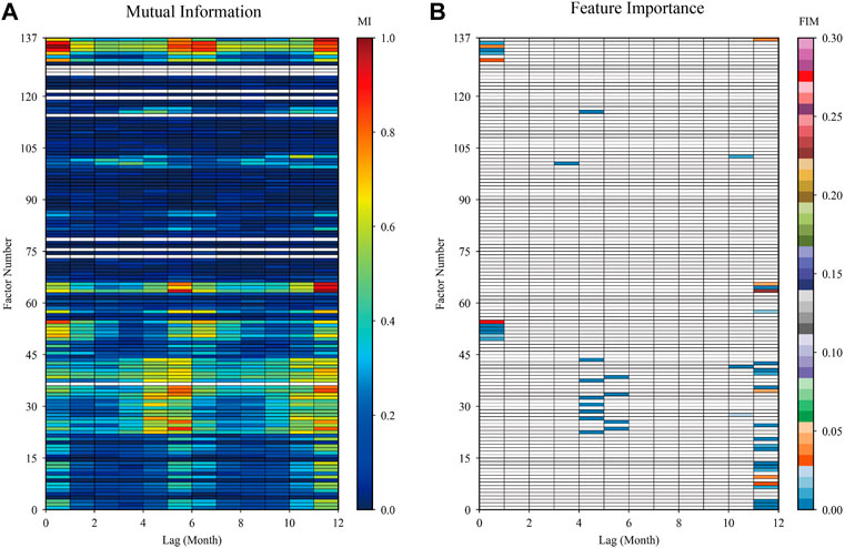
FIGURE 3. the mutual information value among the 137 factors and the observed runoff at a lag of 1–12 months, and the blanks are missing factors (A), and the importance score of the physical factors whose mutual information values are ranked in the top 50, which are filled with color (B).
In this study, we synthesized 10 scenarios (Figure 2) for 4 prediction models, that is HKSVM (M1), ELM (M2), GRNN (M3), and MLR (M4). Thus, four metrics, namely NSE, KGE, RMSE and R, are used to find the optimal input scenario for each model. According to the level of MI (Figure 3A), we selected the top 50 physical factors, and then RF is used to order the importance of these factors (Figure 3B). Based on the order of importance, we sequentially added 5 physical factors each time as the model input. So, a total of 10 input scenarios was generated (Figure 2). Synthesizing the prediction accuracy of the four regression models under 10 input scenarios, the HKSVM and MLR perform best in scenario 4, and the ELM and GRNN perform best in scenario 3. It can be seen from Figure 4 that with the increase of input features, the prediction accuracy of each model firstly becomes better, but after the optimal input scenario appears, increasing the input features is not conducive to further improve the prediction accuracy. There are two main reasons for this result: 1) the input features are too few to reveal the complex variation mechanism of runoff, but the increase the number of input features will introduce some redundant features; 2) if the number of input features are too large, it will increase the observation error of samples and the complexity of the model, which is not good for training the model and could weaken its promotion potential. Therefore, this study adopted the method of gradually increasing the number of input features in order of the feature importance, and selected the best predictors set according to the performance of each model during the testing period.
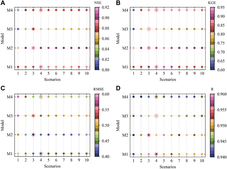
FIGURE 4. The results of NSE (A), KGE (B), RMSE (C), and R (D) of each model for 10 input scenarios. The best input scenario is selected by the red circle. The models represented by M1-M4 are shown in Table 2.
The statistical results of the prediction accuracy evaluation indicators of each model during the training period and the testing period were summarized in Table 2. The training period is the learning phase of the model, and the quality of the learning will directly affect the actual runoff prediction effect. In practical engineering, the performance of the model during the testing phase is usually more concerned, because it reflects the generalization ability and practical application effect of the model. As shown in Table 2, the overall performance of FIA-ML models showed better during the testing period, compared with the runoff time series analysis models. Furthermore, among the FIA-ML models, HKSVM and ELM have better runoff forecasting ability, which further demonstrates that choosing an appropriate machine learning algorithm is also a way to improve the accuracy of runoff prediction. Besides, we can see that GRNN is the best model during the training period, but its performance is not good enough during the testing period. Obviously, GRNN shows overfitting, which is because GRNN is too sensitive to the samples appearing in the learning stage, resulting in the lack of ability to explore the general variation of out-of-sample data. In contrast, HKSVM combines the advantages of polynomial kernel and Gaussian radial basis kernel function, and has relatively strong learning ability and generalization ability. To further compare the effect of each model in practical application, we show the fitting quality of each model during the testing period Figures 5,6,7,8.
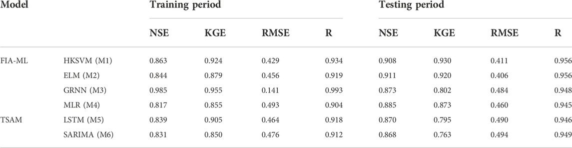
TABLE 2. Prediction accuracy evaluation metrics of different models during training and testing period.
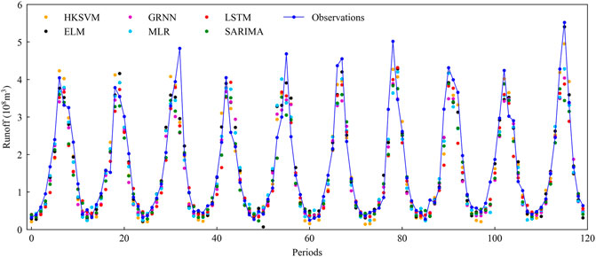
FIGURE 5. Comparison of observed and fitted runoff by different models for 2007–2016 (testing period).
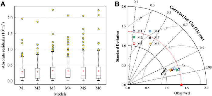
FIGURE 6. Boxplot of absolute residuals (A) and Taylor diagrams (B) of the results of monthly runoff prediction during the testing period. The models represented by M1–M6 are shown in Table 2.
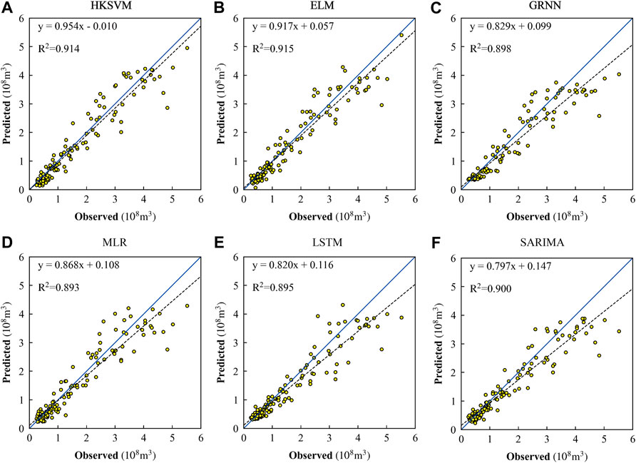
FIGURE 7. Scatter plot of observations and predictions by HKSVM (A), ELM (B), GRNN (C), MLR (D), LSTM (E), and SARIMA (F) during the testing period.
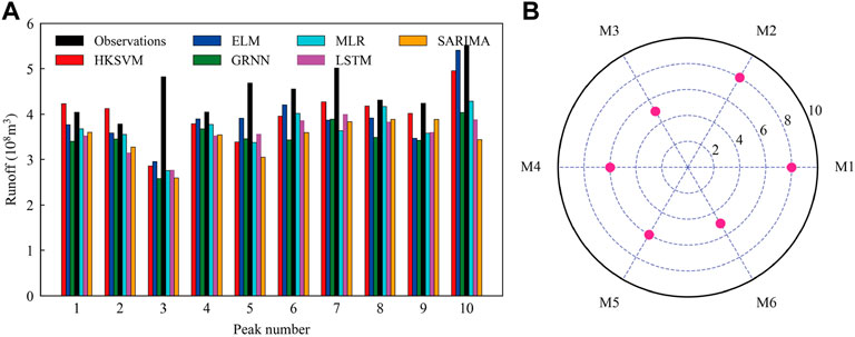
FIGURE 8. Observations and predictions of peak monthly runoff with different models during the testing period are displayed in (A), and the number of years that the predictions of each model meet the design requirements is displayed in (B). The models represented by M1-M6 are shown in Table 2.
Figure 5 shows the fitting performance of the 120-month runoff observations and the predictions of the monthly runoff prediction models during the testing simulation phase. The monthly runoff of YLX during the wet season fluctuates obviously across different years. The FIA-ML models can relatively better capture the variation of monthly runoff, especially with HKSVM and ELM regression models.
Figure 6A is a boxplot of absolute residuals, which can describe the distribution of the difference between the predicted and observed values. Figure 6B is a Taylor diagram (Taylor, 2001), which skillfully integrates the correlation coefficient, centered root mean square error, and standard deviation into a polar plot, avoiding the limitations of a single evaluation metric. Therefore, it can more intuitively show the difference between the predicted and observed values. One can see from Figure 6 that the simulation prediction results of M1 (HKSVM) and M2 (ELM) are closer to the actual runoff observations. This indicated that ELM and HKSVM have more robust capabilities to reveal the correlation between predictors and observed runoff.
Figure 7 shows the linear relationship between the observed runoff and the simulated value obtained by different prediction methods during the testing period. It is found that both the FIA-ML models and the runoff time series analysis models are feasible in tracking the dynamic changes of monthly runoff. In addition, ELM has the best effect from the perspective of
In practical engineering, the prediction accuracy of peak monthly runoff is more significant than runoff in other months. For this reason, we compared the prediction effect of each model on peak monthly runoff during the testing period. According to the standard for hydrological information and hydrological forecasting formulated by the Ministry of Water Resources of China, for medium and long-term runoff prediction, when the relative error of the prediction result is less than 20%, it is considered a valid prediction value (Zhang et al., 2011). As displayed in Figure 8, M1 (HKSVM) and M2 (ELM) have eight years to meet the design requirements, but the performance of M3 (GRNN) and M6 (SARIMA) are relatively poor, with only five years to meet the design requirements.
When using ML for runoff prediction, the choice of predictors is critical. Because the quality of the effective information carried by the features will directly affect the accuracy of runoff prediction. Our simulations revealed that appropriately increasing the number of features can improve the accuracy of monthly runoff prediction. However, too many input features will increase the complexity of training the model and reduce the ability to capture the general changing characteristics of runoff process. In this study, the NSEs of FIA-ML models (M1-M4) were initially 0.878, 0.866, 0.815, and 0.818. When the optimal number of input features for each model was reached, their NSEs were improved by 3.4%, 5.2%, 7.1%, and 8.2%, respectively. However, if the number of input features continue to increase, the accuracy of runoff prediction will not continue to get better. This should be mainly because too many inputs will make the model training subject to some abnormal information interference, and reduce the training efficiency.
Although RF is an effective tool to measure the feature importance, it also has some shortcomings. One of the most important issues is that if there are too many input features in RF, the efficiency and accuracy of calculating the importance score of each feature will be affected. Thus, this study first uses MI to select the top 50 factors related to the observed runoff, which is equivalent to a rough screening from numerous possible factors. The method combined RF with MI can effectively overcome the shortcomings of the single use RF or MI to select predictors as the inputs of the ML models.
Compared with the TSAM, the FIA-ML model can improve the NSE by up to 5%, and more importantly, can explain the variation characteristics of runoff from the physical meaning. However, it should be noted that although the FIA-ML models can improve the prediction accuracy to a certain extent, some issues should be noted in the application. One is that the meteorological information we used is relatively less in this study, so, in future work, we can further consider more meteorological factors related to prediction of monthly runoff. Another is that although the IPSO can effectively improve the global search ability of particles, there is still the problem of falling into local convergence, so it is necessary to explore a more efficient methods for improving the global search ability in selecting model hyper-parameters. In addition, simply depending on the correlation between the runoff process and these physical factors is not enough to fully reveal the variation characteristics of runoff, since the runoff prediction system is open and complex. Therefore, the system dynamics characteristics of the runoff process can be considered in machine learning in further studies.
We proposed the model by combining ML with the feature importance analysis (FIA-ML), which can select key predictors from the numerous physical factors and effectively integrate hydrometeorological information and teleconnection climate factors into the ML models. This paper verified the applicability of the model in the YLX basin, and compared with the traditional time series analysis model (TSAM). Under changing environments, the TSAM cannot accurately capture the impact of climate change on the characteristics of runoff variability. By contrast, the FIA-ML models not only have better runoff prediction ability, but can, more importantly, explain which physical factors have a significant impact on the runoff in the YLX basin.
The FIA-ML models can effectively improve the learning efficiency of ML models and the accuracy of runoff prediction. Especially, HKSVM and ELM optimized by IPSO have a good fitting ability for the relationship between observed runoff and input predictors. Therefore, the FIA-ML model is a useful attempt to improve the accuracy of runoff prediction by establishing the teleconnection between climate change and runoff change.
The original contributions presented in the study are included in the article/Supplementary Material, further inquiries can be directed to the corresponding author.
LY: conceptualization, formal analysis, writing-original draft, writing-review and editing, supervision. QL: methodology, writing-original draft, writing-review, and editing. CJ: writing-original draft. PY: writing-review and editing. BL: writing-review and editing. ZR: writing-review and editing. ZL: writing-review and editing.
This study is financially supported jointly by the National Natural Science Foundation of China (No. 51909053, U2240201, 51909112), the Youth Foundation of Education Department of Hebei Province (QN2019132), Xingtai City Science and Technology Bureau (2021ZZ032), all of which are greatly appreciated.
We are very grateful to the editors and reviewers for their critical comments and thoughtful suggestions.
The authors declare that the research was conducted in the absence of any commercial or financial relationships that could be construed as a potential conflict of interest.
All claims expressed in this article are solely those of the authors and do not necessarily represent those of their affiliated organizations, or those of the publisher, the editors and the reviewers. Any product that may be evaluated in this article, or claim that may be made by its manufacturer, is not guaranteed or endorsed by the publisher.
Bian, Y., Sun, P., Zhang, Q., Luo, M., and Liu, R. (2022). Amplification of non-stationary drought to heatwave duration and intensity in eastern China: Spatiotemporal pattern and causes. J. Hydrol. X. 612, 128154. doi:10.1016/j.jhydrol.2022.128154
Elkiran, G., Nourani, V., Elvis, O., and Abdullahi, J. (2021). Impact of climate change on hydro-climatological parameters in North Cyprus: Application of artificial intelligence-based statistical downscaling models. J. Hydroinform. 23 (6), 1395–1415. doi:10.2166/hydro.2021.091
Fang, W., Huang, S., Huang, Q., Huang, G., Meng, E., and Luan, J. (2018). Reference evapotranspiration forecasting based on local meteorological and global climate information screened by partial mutual information. J. Hydrol. X. 561, 764–779. doi:10.1016/j.jhydrol.2018.04.038
Feng, Z., Liu, S., Niu, W., Li, S., Wu, H., and Wang, J. (2020a). Ecological operation of cascade hydropower reservoirs by elite-guide gravitational search algorithm with Lévy flight local search and mutation. J. Hydrol. X. 581, 124425. doi:10.1016/j.jhydrol.2019.124425
Feng, Z., Niu, W., Tang, Z., Jiang, Z., Yang, X., Liu, Y., et al. (2020b). Monthly runoff time series prediction by variational mode decomposition and support vector machine based on quantum-behaved particle swarm optimization. J. Hydrol. X. 583, 124627. doi:10.1016/j.jhydrol.2020.124627
Genuer, R., Poggi, J. M., and Tuleau-Malot, C. (2010). Variable selection using random forests. Pattern Recognit. Lett. 31 (14), 2225–2236. doi:10.1016/j.patrec.2010.03.014
Ghose, D. K., Mahakur, V., and Sahoo, A. (2022). “Monthly runoff prediction by hybrid CNN-LSTM model: A case study,” in Communications in computer and information science (Cham: Springer), 1614. doi:10.1007/978-3-031-12641-3_31
Gupta, H. V., Kling, H., Yilmaz, K. K., and Martinez, G. F. (2009). Decomposition of the mean squared error and NSE performance criteria: Implications for improving hydrological modelling. J. Hydrol. X. 377 (1-2), 80–91. doi:10.1016/j.jhydrol.2009.08.003
Hapfelmeier, A., Hothorn, T., Ulm, K., and Strobal, C. (2014). A new variable importance measure for random forests with missing data. Stat. Comput. 24 (1), 21–34. doi:10.1007/s11222-012-9349-1
He, X., Guan, H., and Qin, J. (2015). A hybrid wavelet neural network model with mutual information and particle swarm optimization for forecasting monthly rainfall. J. Hydrol. X. 527, 88–100. doi:10.1016/j.jhydrol.2015.04.047
Hu, Y., Liang, Z., Huang, Y., Yao, Y., Wang, J., and Li, B. (2022). A nonstationary bivariate design flood estimation approach coupled with the most likely and expectation combination strategies. J. Hydrol. X. 605, 127325. doi:10.1016/j.jhydrol.2021.127325
Huang, G., Zhu, Q., and Siew, C. K. (2006). Extreme learning machine: Theory and applications. Neurocomputing 70 (1–3), 489–501. doi:10.1016/j.neucom.2005.12.126
Huang, S., Chang, J., Huang, Q., and Chen, Y. (2014). Monthly streamflow prediction using modified EMD-based support vector machine. J. Hydrol. X. 511, 764–775. doi:10.1016/j.jhydrol.2014.01.062
Huang, S., Li, P., Huang, Q., Leng, G., Hou, B., and Ma, L. (2017). The propagation from meteorological to hydrological drought and its potential influence factors. J. Hydrol. X. 547, 184–195. doi:10.1016/j.jhydrol.2017.01.041
Jian, S., Yin, C., Wang, Y., Yu, X., and Li, Y. (2022). The possible incoming runoff under extreme rainfall event in the Fenhe river basin. Front. Environ. Sci. 10, 812351. doi:10.3389/fenvs.2022.812351
Jiang, C., Xiong, L., Yan, L., Dong, J., and Xu, C.-Y. (2019). Multivariate hydrologic design methods under nonstationary conditions and application to engineering practice. Hydrol. Earth Syst. Sci. 23 (3), 1683–1704. doi:10.5194/hess-23-1683-2019
Kraskov, A., Stӧgbauer, H., and Grassberger, P. (2004). Estimating mutual information. Phys. Rev. E 69 (6), 066138. doi:10.1103/PhysRevE.69.066138
Lei, Q., Yan, L., Lu, D., Bu, J., and Luo, Y. (2022). Research on P-III distribution maximum likelihood estimation based on particle swarm optimization algorithm. Chin. Rur. Water Hydropow. 2022 (7), 128–131+139.
Lima, C. H. R., and Lall, U. (2010). Spatial scaling in a changing climate: A hierarchical bayesian model for non-stationary multi-site annual maximum and monthly streamflow. J. Hydrol. X. 383 (3-4), 307–318. doi:10.1016/j.jhydrol.2009.12.045
Lin, K., Sheng, S., Zhou, Y., Liu, F., Li, Z., Chen, H., et al. (2020). The exploration of a Temporal Convolutional Network combined with Encoder-Decoder framework for runoff forecasting. Hydrol. Res. 51 (5), 1136–1149. doi:10.2166/nh.2020.100
Lu, F., Song, X., Xiao, W., Zhu, K., and Xie, Z. (2020). Detecting the impact of climate and reservoirs on extreme floods using nonstationary frequency models. Stoch. Environ. Res. Risk Assess. 34 (1), 169–182. doi:10.1007/s00477-019-01747-2
Luo, K., Tao, F., Deng, X., and Moiwo, J. P. (2017). Changes in potential evapotranspiration and surface runoff in 1981–2010 and the driving factors in Upper Heihe River Basin in Northwest China. Hydrol. Process. 31 (1), 90–103. doi:10.1002/hyp.10974
Ma, Z., Sun, P., Zhang, Q., Zou, Y., Lv, Y., Li, H., et al. (2022). The characteristics and evaluation of future droughts across China through the CMIP6 multi-Model ensemble. Remote Sens. (Basel). 14 (5), 1097. doi:10.3390/rs14051097
Maity, R., and Kashid, S. S. (2011). Importance analysis of local and global climate inputs for basin-scale streamflow prediction. Water Resour. Res. 47 (11), W11504. doi:10.1029/2010WR009742
Mann, H. B. (1945). Nonparametric tests against trend. Econometrica 13 (3), 245–259. doi:10.2307/1907187
Meng, E., Huang, S., Huang, Q., Fang, W., Wu, L., and Wang, L. (2019). A robust method for non-stationary streamflow prediction based on improved EMD-SVM model. J. Hydrol. X. 568, 462–478. doi:10.1016/j.jhydrol.2018.11.015
Niu, W., Feng, Z., Chen, Y., Zhang, H., and Wang, L. (2020). Annual streamflow time series prediction using extreme learning machine based on gravitational search algorithm and variational mode decomposition. J. Hydrol. Eng. 25 (5), 04020008. doi:10.1061/(ASCE)HE.1943-5584.0001902
Niu, W., Feng, Z., Feng, B., Xu, Y., and Min, Y. (2021). Parallel computing and swarm intelligence based artificial intelligence model for multi-step-ahead hydrological time series prediction. Sustain. Cities Soc. 66, 102686. doi:10.1016/j.scs.2020.102686
Nugent, K. A., and Matthews, H. D. (2012). Drivers of future northern latitude runoff change. Atmosphere-Ocean 50 (2), 197–206. doi:10.1080/07055900.2012.658505
Ouyang, Y., Grace, J. M., Parajuli, P. B., and Caldwell, P. V. (2022). Impacts of multiple hurricanes and tropical storms on watershed hydrological processes in the Florida panhandle. Climate 10 (3), 42. doi:10.3390/cli10030042
Peters, D. L., Atkinson, D., Monk, W. A., Tenenbaum, D. E., and Baird, D. J. (2013). A multi-scale hydroclimatic analysis of runoff generation in the Athabasca River, Western Canada. Hydrol. Process. 27 (13), 1915–1934. doi:10.1002/hyp.9699
Samantaray, S., Das, S. S., Sahoo, A., and Satapathy, D. P. (2022a). Monthly runoff prediction at Baitarani river basin by support vector machine based on Salp swarm algorithm. Ain Shams Eng. J. 13 (5), 101732. doi:10.1016/j.asej.2022.101732
Samantaray, S., Sah, M. K., Chalan, M. M., Sahoo, A., and Mohanta, N. R. (2022b). “Runoff prediction using hybrid SVM-PSO approach,” in Lecture notes in networks and systems (Singapore: Springer), 446. doi:10.1007/978-981-19-1559-8_29
Samantaray, S., Sahoo, A., Das, S. S., and Satapathy, D. P. (2022c). Development of rainfall-runoff model using anfis with an integration of gis: A case study. Curr. Dir. Water Scarcity Res. 7, 201–223. doi:10.1016/B978-0-323-91910-4.00013-3
Sharifi, A., Dinpashoh, Y., and Mirabbasi, R. (2017). Daily runoff prediction using the linear and non-linear models. Water Sci. Technol. 76 (4), 793–805. doi:10.2166/wst.2017.234
Sharma, A. (2000). Seasonal to interannual rainfall probabilistic forecasts for improved water supply management: Part 1-A strategy for system predictor identification. J. Hydrol. X. 239 (1- 4), 232–239. doi:10.1016/S0022-1694(00)00346-2
Shi, X., Huang, Q., and Li, K. (2021). Decomposition-based teleconnection between monthly streamflow and global climatic oscillation. J. Hydrol. X. 602, 126651. doi:10.1016/j.jhydrol.2021.126651
Singh, V. K., and Roxy, M. K. (2022). A review of ocean-atmosphere interactions during tropical cyclones in the north Indian Ocean. Earth. Sci. Rev. 226, 103967. doi:10.1016/j.earscirev.2022.103967
Sit, M., Demiray, B. Z., Xiang, Z., Ewing, Y. S., and Demir, I. (2020). A comprehensive review of deep learning applications in hydrology and water resources. Water Sci. Technol. 82 (12), 2635–2670. doi:10.2166/wst.2020.369
Song, X., Lu, F., Wang, H., Xiao, W., and Zhu, K. (2018). Penalized maximum likelihood estimators for the nonstationary Pearson type 3 distribution. J. Hydrol. X. 567, 579–589. doi:10.1016/j.jhydrol.2018.10.035
Soper, D. S. (2021). Greed Is Good: Rapid hyperparameter optimization and model selection using greedy k-fold cross validation. Electronics 10 (16), 1973. doi:10.3390/electronics10161973
Steinschneider, S., and Lall, U. (2016). Spatiotemporal structure of precipitation related to tropical moisture exports over the eastern United States and its relation to climate teleconnections. J. Hydrometeorol. 17 (3), 897–913. doi:10.1175/JHM-D-15-0120.1
Sun, A. Y., Wang, D., and Xu, X. (2014). Monthly streamflow forecasting using Gaussian process regression. J. Hydrol. X. 511, 72–81. doi:10.1016/j.jhydrol.2014.01.023
Sun, P., Ma, Z., Zhang, Q., Singh, V. P., and Xu, C-Y. (2022). Modified drought severity index: Model improvement and its application in drought monitoring in China. J. Hydrol. X. 612, 128097. doi:10.1016/j.jhydrol.2022.128097
Sun, P., Wen, Q., Zhang, Q., Singh, V. P., Sun, Y., and Li, J. (2018). Nonstationarity-based evaluation of flood frequency and flood risk in the Huai River basin, China. J. Hydrol. X. 567, 393–404. doi:10.1016/j.jhydrol.2018.10.031
Talaee, P. H., Tabari, H., and Ardakani, S. S. (2014). Hydrological drought in the west of Iran and possible association with large-scale atmospheric circulation patterns. Hydrol. Process. 28 (3), 764–773. doi:10.1002/hyp.9586
Tang, J., Li, Q., and Chen, J. (2018). Summertime runoff variations and their connections with Asian summer monsoons in the Yangtze River basin. J. Water Clim. Chang. 9 (1), 89–100. doi:10.2166/wcc.2017.142
Taormina, R., and Chau, K. W. (2015). Data-driven input variable selection for rainfall–runoff modeling using binary-coded particle swarm optimization and extreme learning machines. J. Hydrol. X. 529, 1617–1632. doi:10.1016/j.jhydrol.2015.08.022
Taylor, K. E. (2001). Summarizing multiple aspects of model performance in a single diagram. J. Geophys. Res. 106 (D7), 7183–7192. doi:10.1029/2000JD900719
Tiwari, A., and Chaturvedi, A. (2022). A hybrid feature selection approach based on information theory and dynamic butterfly optimization algorithm for data classification. Expert Syst. Appl. 196, 116621. doi:10.1016/j.eswa.2022.116621
Valipour, M. (2015). Long-term runoff study using SARIMA and ARIMA models in the United States. Mater. Apps. 22 (3), 592–598. doi:10.1002/met.1491
Wang, J., Wang, X., Lei, X., Wang, H., Zhang, X., You, J., et al. (2020). Teleconnection analysis of monthly streamflow using ensemble empirical mode decomposition. J. Hydrol. X. 582, 124411. doi:10.1016/j.jhydrol.2019.124411
Wang, W., Yang, P., Xia, J., Zhang, S., and Cai, W. (2022). Coupling analysis of surface runoff variation with atmospheric teleconnection indices in the middle reaches of the Yangtze River. Theor. Appl. Climatol. 148 (3-4), 1513–1527. doi:10.1007/s00704-022-04013-8
Wen, X., Feng, Q., Deo, R. C., Wu, M., Yin, Z., Yang, L., et al. (2019). Two-phase extreme learning machines integrated with the complete ensemble empirical mode decomposition with adaptive noise algorithm for multi-scale runoff prediction problems. J. Hydrol. X. 570, 167–184. doi:10.1016/j.jhydrol.2018.12.060
Xiong, L., Yan, L., Du, T., Yan, P., Li, L., and Xu, W. (2019). Impacts of climate change on urban extreme rainfall and drainage infrastructure performance: A case study in wuhan city, China. Irrig. Drain. 68 (2), 152–164. doi:10.1002/ird.2316
Yan, L., Xiong, L., Jiang, C., Zhang, M., Wang, D., and Xu, C-Y. (2021a). Updating intensity–duration–frequency curves for urban infrastructure design under a changing environment. WIREs Water 8 (3), e1519. doi:10.1002/wat2.1519
Yan, L., Xiong, L., Luan, Q., Jiang, C., Yu, K., and Xu, C-Y. (2020). On the applicability of the expected waiting time method in nonstationary flood design. Water Resour. manage. 34, 2585–2601. doi:10.1007/s11269-020-02581-w
Yan, L., Xiong, L., Ruan, G., Zhang, M., and Xu, C-Y. (2021b). Design flood estimation with varying record lengths in Norway under stationarity and nonstationarity scenarios. Hydrol. Res. 52 (6), 1596–1614. doi:10.2166/nh.2021.026
Yang, P., Xia, J., Luo, X., Meng, L., Zhang, S., Cai, W., et al. (2021). Impacts of climate change-related flood events in the Yangtze River Basin based on multi-source data. Atmos. Res. 263, 105819. doi:10.1016/j.atmosres.2021.105819
Yang, T., Asanjan, A. A., Welles, E., Gao, X., Sorooshian, S., and Liu, X. (2017). Developing reservoir monthly inflow forecasts using artificial intelligence and climate phenomenon information. Water Resour. Res. 53 (4), 2786–2812. doi:10.1002/2017WR020482
You, Y., Liu, J., Zhang, Y., Beck, H. E., Gu, H., and Kong, D. (2021). Impacts of El Niño–southern oscillation on global runoff: Characteristic signatures and potential mechanisms. Hydrol. Process. 35 (10), e14367. doi:10.1002/hyp.14367
Yuan, X., Chen, C., Lei, X., Yuan, Y., and Adnan, R. M. (2018). Monthly runoff forecasting based on LSTM–ALO model. Stoch. Environ. Res. Risk Assess. 32 (8), 2199–2212. doi:10.1007/s00477-018-1560-y
Zhang, Q., Wang, B., He, B., Peng, Y., and Ren, M. (2011). Singular spectrum analysis and ARIMA hybrid model for annual runoff forecasting. Water Resour. manage. 25 (11), 2683–2703. doi:10.1007/s11269-011-9833-y
Zhao, X., Lv, H., Lv, S., Sang, Y., Wei, Y., and Zhu, X. (2021). Enhancing robustness of monthly streamflow forecasting model using gated recurrent unit based on improved grey wolf optimizer. J. Hydrol. X. 601, 126607. doi:10.1016/j.jhydrol.2021.126607
Zheng, S., Liu, J., and Tian, J. (2005). An efficient star acquisition method based on SVM with mixtures of kernels. Pattern Recognit. Lett. 26 (2), 147–165. doi:10.1016/j.patrec.2004.09.003
Zhou, X., Chen, W., Liu, Q., Shen, H., Cai, S., and Lei, X. (2022). Future runoff forecast in Hanjiang River Basin based on Wetspa model and CMIP6 model. Front. Environ. Sci. 10, 980949. doi:10.3389/fenvs.2022.980949
Zhou, X., Jiang, P., and Wang, X. (2018). Recognition of control chart patterns using fuzzy SVM with a hybrid kernel function. J. Intell. Manuf. 29 (1), 51–67. doi:10.1007/s10845-015-1089-6
Zou, Y., Sun, P., Ma, Z., Lv, Y., and Zhang, Q. (2022). Snow cover in the three stable snow cover areas of China and spatio-temporal patterns of the future. Remote Sens. (Basel). 14 (13), 3098. doi:10.3390/rs14133098
Keywords: runoff prediction, mutual information, random forest, feature importance analysis, teleconnection
Citation: Yan L, Lei Q, Jiang C, Yan P, Ren Z, Liu B and Liu Z (2022) Climate-informed monthly runoff prediction model using machine learning and feature importance analysis. Front. Environ. Sci. 10:1049840. doi: 10.3389/fenvs.2022.1049840
Received: 21 September 2022; Accepted: 03 November 2022;
Published: 17 November 2022.
Edited by:
Peng Sun, Anhui Normal University, ChinaReviewed by:
Yanlai Zhou, Wuhan University, ChinaCopyright © 2022 Yan, Lei, Jiang, Yan, Ren, Liu and Liu. This is an open-access article distributed under the terms of the Creative Commons Attribution License (CC BY). The use, distribution or reproduction in other forums is permitted, provided the original author(s) and the copyright owner(s) are credited and that the original publication in this journal is cited, in accordance with accepted academic practice. No use, distribution or reproduction is permitted which does not comply with these terms.
*Correspondence: Lei Yan, eWFubEB3aHUuZWR1LmNu
Disclaimer: All claims expressed in this article are solely those of the authors and do not necessarily represent those of their affiliated organizations, or those of the publisher, the editors and the reviewers. Any product that may be evaluated in this article or claim that may be made by its manufacturer is not guaranteed or endorsed by the publisher.
Research integrity at Frontiers
Learn more about the work of our research integrity team to safeguard the quality of each article we publish.