
94% of researchers rate our articles as excellent or good
Learn more about the work of our research integrity team to safeguard the quality of each article we publish.
Find out more
ORIGINAL RESEARCH article
Front. Environ. Sci., 21 October 2022
Sec. Environmental Informatics and Remote Sensing
Volume 10 - 2022 | https://doi.org/10.3389/fenvs.2022.1044839
 Yanzhou Li1†
 Feng Qin1,2†Yanzhou He1,2†
 Bo Liu2Conghui Liu2Xuejiao Pu2
 Fanghao Wan2*
 Xi Qiao1,2*
 Wanqiang Qian2*
The invasion of Spartina alterniflora (S. alterniflora) has resulted in significant losses in the diversity of coastal ecosystems. However, the impact of seasonal changes on the accurate identification of S. alterniflora remains to be explored, which is of great significance due to its early monitoring and warning. In this study, S. alterniflora in Beihai, Guangxi, was selected as the research object. Unmanned aerial vehicles (UAVs) and deep convolutional neural networks (CNNs) were used to explore the identification of S. alterniflora in different seasons. Through comparative analysis, the ResNet50 model performed well in identifying S. alterniflora, with an F1-score of 96.40%. The phenological characteristics of S. alterniflora differ in different seasons. It is difficult to accurately monitor the annual S. alterniflora using only single-season data. For the monitoring of S. alterniflora throughout the year, the autumn-winter two-season model was selected from the perspective of time cost, the four-season model was selected from the perspective of identification performance, and the three-season model of summer, autumn and winter was selected from the perspective of time cost and identification performance. In addition, a method was developed to predict and evaluate the diffusion trend of S. alterniflora based on time series UAV images. Using the spring data to predict the diffusion trend of S. alterniflora in summer and autumn, the results showed that the highest recall reached 84.28%, the F1-score was higher than 70%, and most of the diffusion of S. alterniflora was correctly predicted. This study demonstrates the feasibility of distinguishing S. alterniflora from native plants in different seasons based on UAV and CNN recognition algorithms. The proposed diffusion early warning method reflects the actual diffusion of S. alterniflora to a certain extent, which is of great significance for the early management of invasive plants in coastal wetlands.
As an important type of biological invasion, plant invasions have become a significant ecological problem, threatening native species and affecting the structure and function of ecosystems (Liu et al., 2018). Spartina alterniflora (S. alterniflora) is a perennial herb native to the Atlantic coast of North America. It has strong adaptability and tolerance to the climate and environment and is generally considered to be beneficial to ecological restoration (Li et al., 2020; Zhang et al., 2020; Zhu et al., 2022). To protect the beach environment, China introduced S. alterniflora from the United States in December 1979 and achieved certain economic benefits during the early stage (Cui et al., 2011; Tian et al., 2020; Yang, 2020). However, once S. alterniflora invades an ecosystem, it quickly becomes a local dominant species, leading to a decrease in biodiversity (Li et al., 2009; Wang et al., 2015; Wang et al., 2021) and a negative impact on the local coastal ecological environment and economic development (An et al., 2007; Ren et al., 2019; Wu et al., 2020; Xu et al., 2021). In 2003, S. alterniflora was categorized as one of the most serious invasive plants by the State Environmental Protection Administration of China (Chung, 2006). In the past, managers have tried to eradicate and contain their effects in the invasion process, but these management measures have been difficult and expensive (Vaz et al., 2018). Recently, early monitoring and warning have been recognized as some of the most cost-effective means of responding to biological invasions (Grosse-Stoltenberg et al., 2018; Martin et al., 2018).
Over the years, scholars have carried out much research on monitoring the invasion of S. alterniflora in coastal areas of China. However, most studies have focused on the monitoring of S. alterniflora in specific seasons, and detailed analysis of its invasion from the perspective of different seasons is rare. (Li et al., 2020). When different researchers use or interpret images from different seasons, the results are often highly uncertain (Zhang et al., 2020). To facilitate the management and control of this invasive plant, an efficient and accurate method for monitoring S. alterniflora in different seasons is needed. Most of the classification methods used to date are traditional machine learning algorithms, such as maximum likelihood, support vector machine, and random forest (Ren et al., 2014; Wang et al., 2015). These methods have a low degree of automation and limited processing capabilities for complex functions, making it difficult to improve the classification accuracy of S. alterniflora in complex backgrounds in the wild. Deep learning is a new field in machine learning that realizes the powerful ability to learn the basic features of data from samples by learning a multilayer nonlinear network structure and transforming the basic properties of the original data into more robust abstract features (Zhu et al., 2022). Hang et al. (2019) used a deep learning method to identify and classify plant leaf diseases and achieved an accuracy of 91.7% on a test dataset, which greatly improved the efficiency and accuracy of identification. Chen et al. (2020) used the SRCNN and FSRCNN to monitor and analyse S. alterniflora at the patch scale, and the results showed that the FSRCNN could more accurately identify S. alterniflora in small patches. A deep convolutional neural network (CNN) can automatically extract features from image data, which greatly improves the classification accuracy in complex environments. However, the current research using CNNs to identify S. alterniflora is limited to a specific season, and whether CNNs can reliably distinguish S. alterniflora and native plants in different seasons remains to be further explored.
S. alterniflora appeared in different states and scales during the invasion process, such as small discrete patches at the early stage of invasion; connected strips, broken patches and mixed patches at the middle stage of invasion; and large single-population patches at the end of invasion. These different states exist simultaneously in any intrusion zone (Zhu et al., 2022). Remote sensing has been shown to be a viable tool for monitoring the dynamics of invasive plants (Lawrence et al., 2006; Bradley, 2014). In the past 10 years, medium-resolution satellites have been widely used in the monitoring of S. alterniflora, which can effectively monitor S. alterniflora in the middle and late stages of invasion (Zuo et al., 2012; O'Donnell and Schalles, 2016). However, even with submeter-level high-resolution satellites, it is difficult to effectively identify the early invasion of S. alterniflora, which is not conducive to early monitoring and warning (Ai et al., 2017; Liu et al., 2017; Zhu et al., 2019). In recent years, UAVs, as a new type of remote sensing platform, have provided unparalleled spatial and temporal resolution at reasonable cost, which provides a new way to accurately monitor S. alterniflora in the early stage of invasion (Martin et al., 2018). S. alterniflora is in the early stage of invasion, and its invasion has not been fully established, which is the best period for its control. UAVs can detect and provide a more detailed distribution map of S. alterniflora over time. The analysis of time-series UAV image data will help us to further understand the diffusion mechanism of S. alterniflora, making it possible to predict the diffusion of S. alterniflora. However, relevant studies on the diffusion prediction of S. alterniflora have not been reported. Achieving accurate identification of S. alterniflora and prediction of its spreading trend will help managers formulate more effective management and containment measures.
In this study, the following questions were discussed: 1) Can a time-series UAV image recognition algorithm based on CNN reliably distinguish S. alterniflora from native plants? 2) Can time-series UAV images based on phenology predict the diffusion of S. alterniflora? As a pilot and methodological study, Beihai, China was selected as the case study area, where S. alterniflora has been expanding and migrating significantly. The specific objectives of this study are 1) to develop and evaluate CNN-based recognition algorithms to effectively distinguish S. alterniflora from native plants using time-series UAV images. 2) Develop a method to predict and evaluate the diffusion trend of S. alterniflora based on time-series UAV images.
The study area was located in Zhulin Village, Yinhai District, Beihai City, Guangxi Zhuang Autonomous Region, China (21°27′43.58″N, 109°18′54.02″E), as shown in Figure 1A. It has a typical subtropical monsoon climate with an annual mean temperature of approximately 23.3°C and annual mean precipitation of approximately 1800 mm. The most common native plants in the study area are mangroves, which play an important role in maintaining the ecological balance of coastal areas, preventing wind damage, and protecting the environment (He et al., 2019). However, S. alterniflora invasion is evident here, and it is squeezing the mangrove habitats.
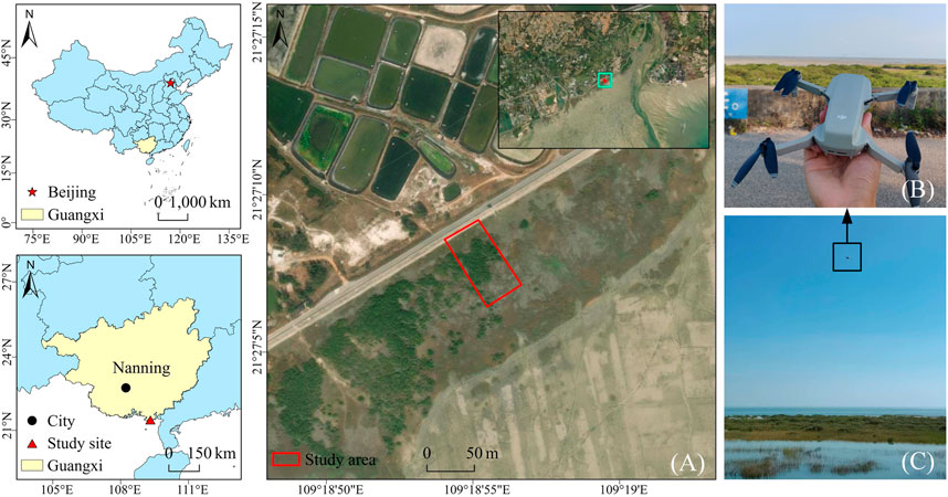
FIGURE 1. Location of the study area and field work scenarios. Among them, (A) shows the study area located in Beihai, Guangxi, China; (B,C) shows the working scene of UAV in the field.
Experimental image data were collected in December 2020 March 2021, June 2021, and September 2021. They are denoted as winter, spring, summer and autumn data. The UAV platform is a DJI Royal MAVIC MINI UAV. The specific parameters are shown in Table 1, and the acquisition equipment and field work scenarios are shown in Figures 1B,C. In the research area, the UAV is 10 m above the ground, the average flight speed is 4.0 m/s, and the pitch angle of the gimbal is -90°. Take equally spaced photos and ensure an image overlap of 60% in both the forward and sideward directions. In each season, 1,200 original images were collected with a spatial resolution of 4,000 × 2,250.
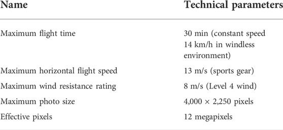
TABLE 1. The major parameters of MAVIC MINI.
After acquiring the original images of the UAV, Agisoft PhotoScan (The Agisoft Inc., Russia) was used to create orthophotos based on the UAV position and direction parameters provided by the UAV inertial system. The orthophotos were cropped to remove parts irrelevant to the experiment, resulting in four seasons of orthophotos with a pixel size of 9,408 × 18,928 (Figures 2A–D).
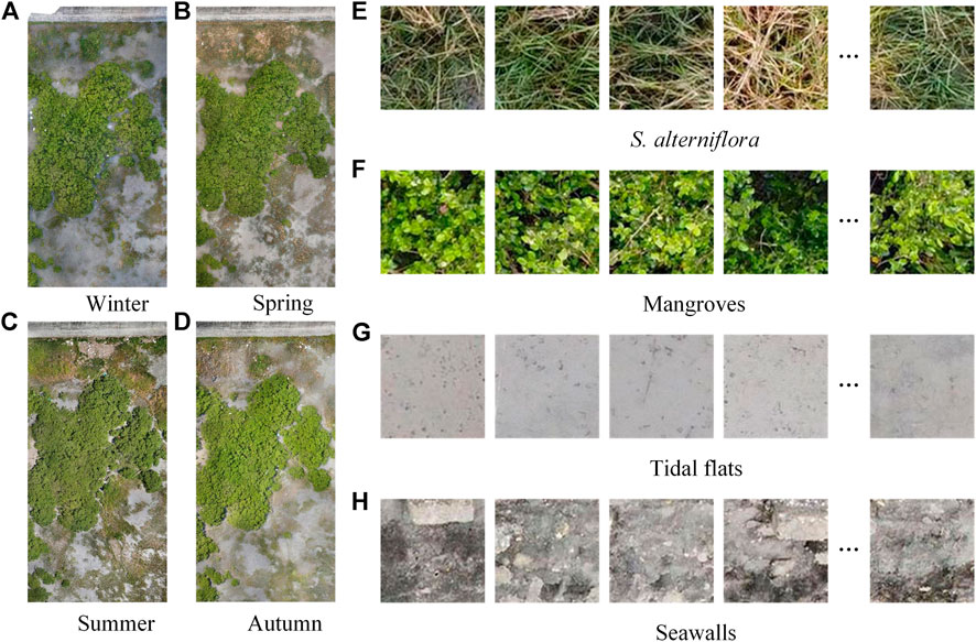
FIGURE 2. Orthophotos and dataset categories. Where (A–D) are orthophotos in winter, spring, summer, and autumn (2020/12, 2021/03, 2021/06, 2021/09); (E–H) are schematic diagrams of S. alterniflora, mangroves, tidal flats, and seawalls.
MATLAB 2018 (The Math Works Inc., United States) was used to segment the orthophoto images, and 14,196 blocks with 112 × 112 pixels were obtained in each season. Then, 14,196 blocks were divided into four categories, including S. alterniflora, mangroves, tidal flats and seawalls (Figures 2E–H). In each season, 4,500 samples were randomly selected from S. alterniflora and mangroves, and 1,500 samples were randomly selected from tidal flats and seawalls to obtain four single-season datasets (AD1-AD4). Two-season (BD1-BD4), three-season (CD1-CD4) and four-season (DD) datasets were obtained through the equal proportion combination of each single-season dataset, and the number of samples of each category in all datasets was consistent (Figure 3). Finally, according to the ratio of 6:2:2, each dataset is divided into a training set, validation set and test set.
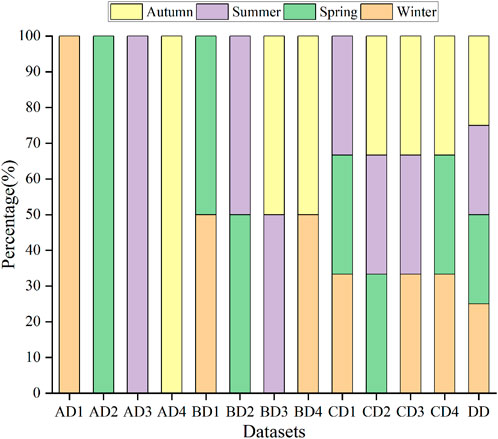
FIGURE 3. The composition of different datasets, in which AD1-AD4 represents winter, spring, summer and autumn datasets, BD1-BD4 represents winter/spring, spring/summer, summer/autumn and autumn/winter combined datasets, CD1-CD4 represents winter/spring/summer, spring/summer/autumn, summer/autumn/winter and autumn/winter/spring combined datasets, and DD represents all season combined dataset.
We use the spring dataset to select one of five deep learning models and train it on all the datasets. The model with the best classification performance for S. alterniflora throughout the year and spring was selected. Then generate an early warning heat map according to the spring classification map of S. alterniflora and the diffusion distance. The specific technical process of this study is shown in Figure 4.
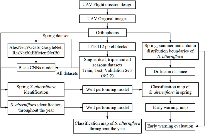
FIGURE 4. Research technical route.
There are many CNN models used for classification tasks in the early stage, such as LeNet, AlexNet, VGG, GoogleNet, ResNet, and DenseNet. Newly released algorithm models in recent years, such as MobileNet, ShuffleNet, EfficientNet, etc. The model is becoming increasingly sophisticated, and the recognition speed and recognition accuracy of the model are increasing. Abade A et al. compiled statistics on 121 papers selected in the past 10 years on the identification of plant pests and diseases, and the results showed that AlexNet, VGG, ResNet, LeNet, Inception V3, and GoogleNet were more commonly used in previous studies (Abade et al., 2021). Therefore, this paper preliminarily selects AlexNet (Krizhevsky et al., 2012), VGG16 (Simonyan and Zisserman, 2014), GoogleNet (Szegedy et al., 2014), ResNet50 (He et al., 2016) and EfficientNetB0 (Tan and Le, 2019), which are frequently used in previous studies and recently published, as the CNN model for identifying S. alterniflora. The parameters of the CNN model used in this paper are based on the parameters of the original paper. According to the classification task, the last part of the network is modified to make the model meet the classification requirements.
In the CNN model, in addition to the structure of the model itself, the learning rate, training epochs, and training batch size will also affect the convergence speed and generalization ability of the model. When the learning rate is too large, the model will easily fall into the local minimum, while when the learning rate is too small, the model will slow down the convergence speed. If the training epochs are set too large, the model training will be slow, and if the training epochs are too small, the model will stop training before convergence, and the optimal result will not be obtained. Within a certain range, the larger the set of train batch sizes, the higher the resource utilization rate of the computer, and the faster the model training speed will be. In this paper, all models are trained with consistent hyperparameter settings. The initial learning rate is 0.01, the learning decay rate is 0.85, the training epochs are 500, and the sample batch size is 128.
The AlexNet (Krizhevsky et al., 2012) network consists of five convolutional layers, three pooling layers, and three fully connected layers. The convolutional layer and the pooling layer are mainly used to extract image feature information, the fully connected layer converts the feature map into a feature vector, and the last fully connected layer submits the output to the Softmax layer. And AlexNet proposed new technologies such as LRN (Local Response Normalization), ReLU activation function, Dropout, and GPU acceleration in model training, which successfully promoted the development of neural networks.
VGGNet (Simonyan and Zisserman, 2014) explores the relationship between the depth of convolutional neural networks and their performance, building deep convolutional neural networks by repeatedly stacking 3 × 3 convolution kernels and 2 × 2 max-pooling layers. VGG16 has 13 convolutional layers and three fully connected layers. The 13 convolutional layers are divided by the Max-pooling layer at the second, fourth, seventh, 10th and 13th layers respectively, which can reduce the length and width of the feature map by 1/2.
GoogleNet (Szegedy et al., 2014) first reduces the number of channels and aggregates information through 1 × 1 convolution, and then performs the calculation, which effectively utilizes the computing power. The fusion of different scales of convolution and pooling operations, as well as the fusion of multi-dimensional features, makes the recognition and classification performance better. Widening the network model structure also avoids the problem of training gradient dispersion caused by the network being too deep. The GoogleNet network adopts global mean pooling, which solves the characteristics of the traditional CNN network that the parameters of the last fully connected layer are too complex and the generalization ability is poor.
ResNet (He et al., 2016) adds a residual unit to the network structure. The residual unit establishes a direct shortcut channel between input and output, implementing an identity mapping layer with the same output as the input. In this way, ResNet solves the problems of gradient dispersion and accuracy degradation in deep networks, which not only ensures the training accuracy, but also controls the training speed.
EfficientNet (Tan and Le, 2019) uses network search techniques to search the network’s input image resolution, depth and width parameters to obtain the most balanced match. Such an efficient network not only has less parameters, but also can learn the deep semantic information of images well, and is more robust for classification tasks.
An important indicator of the diffusion prediction of S. alterniflora is the diffusion distance in a certain period. A part of the distribution map of S. alterniflora in spring was randomly selected and divided into three equal parts. Using manual annotation, the distribution contours of S. alterniflora in spring, summer and autumn were marked (Figure 5).
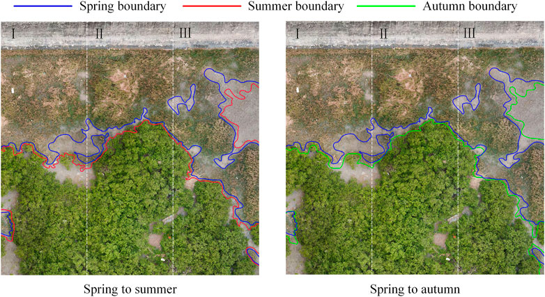
FIGURE 5. The actual distribution profile of S. alterniflora.
Then, set the borderline width to one pixel and count the spring-summer and spring-autumn borderline pixels and the spring-summer and spring-autumn diffusion area pixels. The diffusion distance H is calculated according to Formula 1, where
For the prediction point O, the probability
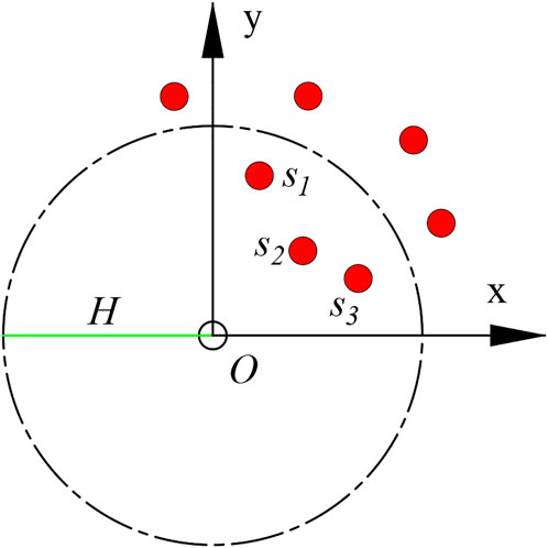
FIGURE 6. Prediction method of S. alterniflora diffusion, in which the red dots indicate the existing distribution of S. alterniflora, O indicates the point to be predicted, H indicates the diffusion distance, and the red dots marked with S indicate the S. alterniflora within the radius H.
In this paper, the recognition effect of the network model and early warning of S. alterniflora diffusion need to be quantitatively evaluated. Accuracy, precision, recall, F1-score, efficiency and K were used as evaluation indicators. The calculation formula of each indicator is as follows:
where A is the accuracy, P is the precision, R is the recall, F is the F1-score, TP is the true positive sample, TN is the true negative sample, FP is the false-positive sample, FN is the false negative sample, E is the efficiency, N is the number of samples in the test set, and
To select the CNN model suitable for S. alterniflora. Recognition, the spring dataset (AD2) was used as the basic dataset for training and testing each model. The training results of the model are obtained, as shown in Figure 7. After 500 epochs of training, the loss tends flatten, and the accuracy of the training set does not rise any more, indicating that all models have reached the convergence state. The highest accuracies of the AlexNet, VGG16, GoogleNet, EfficientNetB0 and ResNet50 models are 84.23%, 93.03%, 96.32%, 94.77% and 98.03%, respectively. Among them, ResNet50 has the highest accuracy and good recognition ability on the training set, while AlexNet has the lowest accuracy.
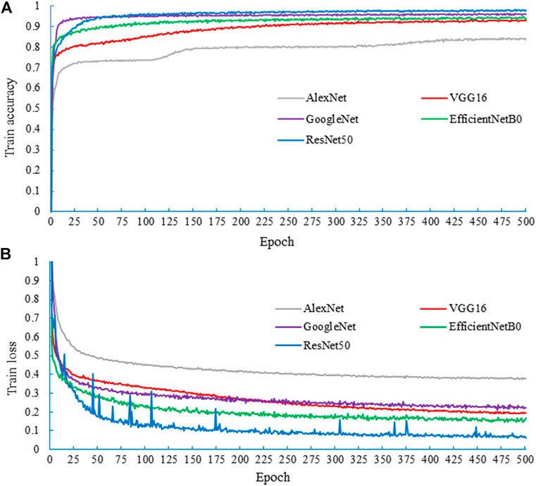
FIGURE 7. The training results of the spring network model, where (A) is the accuracy of the training process and (B) is the loss of the training process.
After all models converge in training, an optimal model will be saved. The test set of the AD2 dataset is fed into each saved model. The accuracy, precision, recall, F1-score and efficiency of each model are calculated, and the results are shown in Table 2.
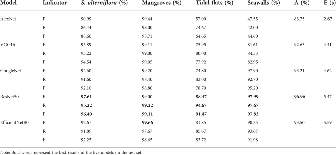
TABLE 2. Test results of five CNN models.
In Table 2, the bold fonts represent the optimal recognition results of the five models on the test set. The total accuracy of ResNet50 was 96.96%, which is much greater than that of the other models. The total accuracy of AlexNet is the lowest, reaching only 83.75%. In the identification of S. alterniflora, ResNet50 achieved a precision of 97.61%, a recall of 95.22%, and an F1-score of 96.40%. Compared with the other four models, ResNet50 had the best classification performance. In the identification of mangroves, EfficientNetB0 has the highest precision of 99.66%. ResNet50 has the best recall (99.22%) and F1-score (99.11%). In addition, in the recognition of tidal flats and seawalls, ResNet50 has the best classification performance among the five models. In terms of efficiency, AlexNet takes the least time, while EfficientNetB0 takes the most time. Considering the total accuracy and efficiency, ResNet50 has a good recognition result for S. alterniflora, so ResNet50 was selected as the recognition model.
First, the training sets of the AD1-DD dataset were fed into ResNet50, and all the trained ResNet50 structures and training hyperparameters were consistent. The trained models were obtained and denoted as A1-D models. Second, the test sets of AD1-AD4 were fed into each trained model to generate a confusion matrix. Then, the accuracy, precision, recall and F1-score of each model for the AD1-AD4 test set were calculated. Finally, the F1-score of S. alterniflora, mangroves, tidal flats and seawalls identified by each model in the four seasons was drawn into a bar chart, and its average value was calculated, as shown in Figure 8.
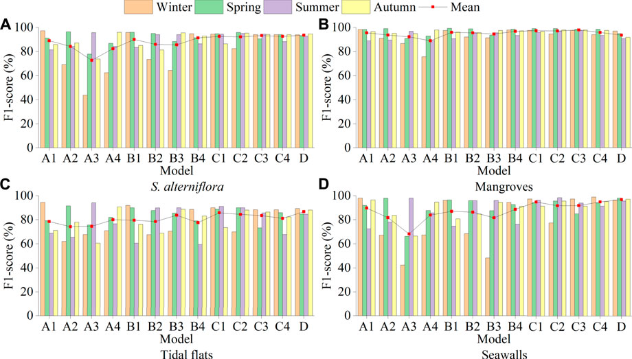
FIGURE 8. (A–D), respectively show the F1-score of each model of S. alterniflora, mangroves, tidal flats and seawalls, where A1-A4 represents the single-season model of winter, spring, summer and autumn, B1-B4 represents the two-season model of winter/spring, spring/summer, summer/autumn and autumn/winter, C1-C4 represents the three-season model of winter/spring/summer, spring/summer/autumn, summer/autumn/winter and autumn/winter/spring, and D represents the four-season model.
The single-season model (A1-A4) was good at identifying S. alterniflora in their respective seasons but poor at identifying S. alterniflora in the other three seasons, indicating that there were differences in the characteristics of S. alterniflora in different seasons (Figure 8A). In the A2, A3 and A4 models, the F1-score of S. alterniflora in winter was lower than 70%, among which the F1-score of the A3 model was only 43.90%, indicating that S. alterniflora in winter was not easy to identify. The mean F1-score of the A1 model was the highest at 89%, and that of the A3 model was the lowest at 72.84%. In different seasons, the characteristics of S. alterniflora that can be learned by CNN are significantly different, so it is difficult to accurately monitor S. alterniflora using only single-season data. The recognition ability of the single-season model for the four seasons of S. alterniflora was A1>A2>A4>A3.
In the two-season model (B1-B4), B2 and B3 recognized S. alterniflora poorly in winter, with F1-scores of 73.48% and 64.39%, respectively. Neither model was trained on winter data, suggesting that winter data play a key role in monitoring S. alterniflora throughout the year. The mean F1-score of the B4 model was the highest at 91.37%, and that of the B3 model was the lowest at 85.57%. The recognition ability of the two-season model for the four seasons of S. alterniflora was B4>B1>B2>B3.
In the three-season models (C1-C4), the C2 model had the best recognition of S. alterniflora in spring, with an F1-score of 95.84%, and the worst recognition of S. alterniflora in winter, with an F1-score of only 82.43%. The F1-score of the C3 model for S. alterniflora identification in the four seasons was above 90.00%, and the mean F1-score was 93.31%. The recognition ability of the three-season model for the four seasons of S. alterniflora was C3>C1>C4>C2. The F1-scores of the four-season D model for S. alterniflora identification in the four seasons were 93.95%, 93.03%, 92.97% and 94.65%, respectively, and the mean F1-score was the highest among all the models, which was 93.65%.
Overall, the ability of different combination models to recognize S. alterniflora throughout the year was D > C3>B4>A1. From the perspective of time cost, the B4 model can be selected as the model to identify S. alterniflora throughout the year. Although the B4 model has a slightly lower recognition accuracy for S. alterniflora in summer, it only uses the data of two seasons, which can save a lot of time. From the perspective of recognition accuracy, the D model can be selected, which has the highest accuracy among all models. From the perspective of time cost and recognition accuracy, the C3 model can be selected as the model to identify S. alterniflora throughout the year.
For the identification of mangroves, the average F1-Score of the C3 three-season model was the largest at 97.83%, while the average F1-Score of the three single-season models of A1-A3 were all above 90%. Overall, no matter which model is used, it can better identify mangroves throughout the year. The characteristics of mangroves in different seasons are similar, and the CNN can use the data from a certain season to accurately identify mangroves throughout the year (Figure 8B). For tidal flat identification, regardless of the model used, as long as the dataset used for training does not contain a dataset of a certain season, the model will not perform well in tidal flat identification in that season. Even if the D model includes data from the four seasons, its average F1-score is still lower than 90%, which may be because in different seasons, the characteristics of tidal flats change greatly under the interference of environmental factors such as sunlight and tides. This will cause great interference in the accurate identification of tidal flats (Figure 8C). For the identification of seawalls, in the single-season model (A1-A4) and the two-season model (B1-B4), except for the A3 model, the average F1-score was 68.26%, and the rest were all higher than 80%. The average F1-score was above 90% in both the C1-C4 and D models, with the D model being the highest at 96.85%. The identification of seawalls was greatly improved by combining multiseason data (Figure 8D).
The F1-score of the D model is the highest, so the D model is selected as the network model for the monitoring of S. alterniflora throughout the year. The colour of the identified S. alterniflora was marked in red to obtain the distribution map of S. alterniflora in different seasons. Intuitively, the general distribution of S. alterniflora in the four seasons is basically consistent with the actual distribution of S. alterniflora (Figures 9A–D). The coverage rate of S. alterniflora in each season was calculated, and it can be seen that the coverage rate of S. alterniflora increased gradually from winter to spring and then to summer, while the coverage rate of S. alterniflora decreased from summer to autumn (Figure 9E).
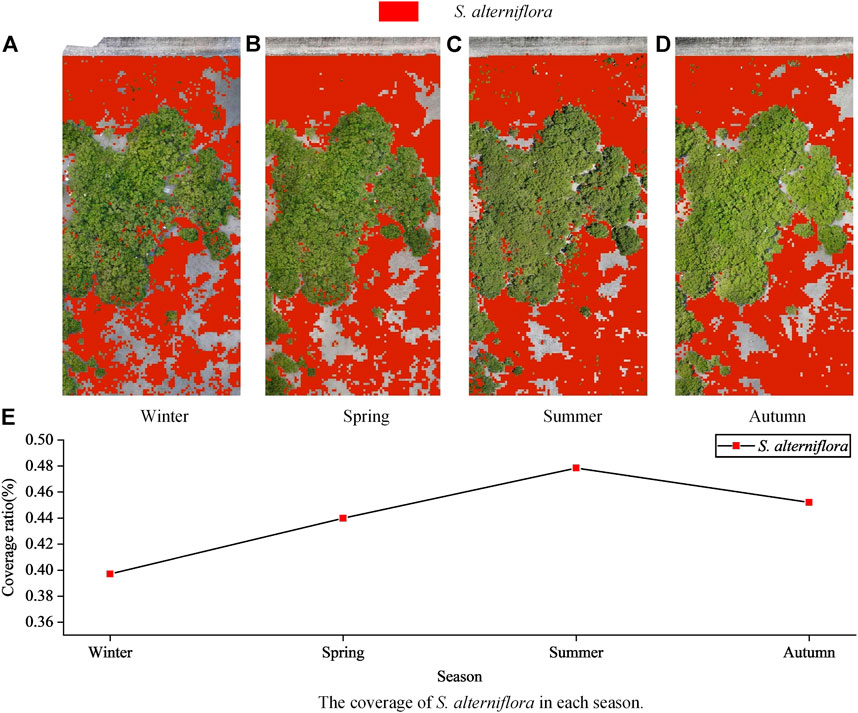
FIGURE 9. (A–D) shows the identification distribution of S. alterniflora in different seasons, and (E) shows the coverage of S. alterniflora in each season.
S. alterniflora mainly diffuses through rhizomes and seeds, and through rhizome diffusion, it expands more stably based on the original distribution, while it is more difficult to accurately capture through seed diffusion. From spring to autumn, S. alterniflora diffusion mainly through rhizomes, and its seeds were immature, which provided the possibility to accurately predict the diffusion of S. alterniflora. In addition, since S. alterniflora is easier to identify in spring, its diffusion from spring to summer and spring to autumn was predicted based on spring S. alterniflora.
Table 3 shows that from summer to autumn, at the boundary of the S. alterniflora distribution, the diffusion area of S. alterniflora in plots I and III further increased, while that in plot II decreased slightly. This result is inconsistent with the decreasing trend of the overall coverage of S. alterniflora. During this period, part of S. alterniflora withered gradually, resulting in a decrease in the overall coverage of S. alterniflora. However, S. alterniflora would continue to diffuse outward, so the diffusion area at the boundary of S. alterniflora would further increase.
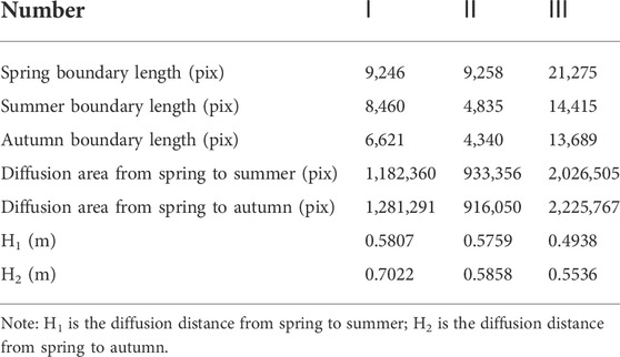
TABLE 3. Statistical value of S. alterniflora diffusion index.
The A2 model had the highest recognition accuracy for S. alterniflora in spring, and the early warning process was based on the distribution map of S. alterniflora in spring. To minimize the impact of misidentification, the A2 model was used to obtain the distribution map of S. alterniflora in spring as the base image.
Ideally, S. alterniflora’s ability to diffuse is the same in all directions and gradually diminishes from the inside out. Take S. alterniflora as the centre point and take the radius H to create a buffer area, where H is the diffusion distance of S. alterniflora calculated above, and gradually fill grey from the centre (the grey value of the centre point) to the boundary (zero). For areas with buffer crossings, greyscale values can be superimposed to generate an early warning heatmap (Figure 10). The blue border represents the border of the early warning result, and the darker the red colour of the area is, the denser S. alterniflora is here. It can be seen intuitively that most of the early warning areas of S. alterniflora are consistent with the actual distribution of S. alterniflora, but there are large deviations in some places.
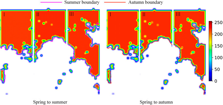
FIGURE 10. Early warning heatmap.
In the early warning map, check the original spring map where there is a large deviation (Figure 11). During the identification of S. alterniflora, the model identified hay as normal S. alterniflora. The hay will not spread further and will be transported to other places with the seawater, thus affecting the early warning of the spread of S. alterniflora. To accurately assess the spread of S. alterniflora early warning, the impact of these hay needs to be removed.
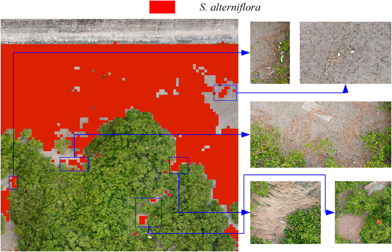
FIGURE 11. The A2 model misidentifies hay as S. alterniflora in spring.
From Table 4, it can be seen that before removing the influence of hay, the K of the three plots was much larger than 1, and the maximum was 1.5242. Their precisions are all lower than 65%, indicating that the area of the diffusion warning is too large. The minimum recall is 74.40%, and the maximum is 84.28%, indicating that the diffusion warning area contains most of the actual diffusion area. After removing the influence of hay, K was closer to 1, and its maximum value was only 1.1787, indicating that the predicted diffusion area of S. alterniflora was closer to the actual diffusion area. The precisions are all greater than 70%, and the maximum value reaches 75.03%. This shows that after removing the influence of hay, the precision has been improved, which is closer to the actual precision of the diffusion warning. The minimum F1-score was 72.87%, and the maximum was 77.37%, indicating that the predicted diffusion area of S. alterniflora reflected the actual spread of S. alterniflora to a certain extent.
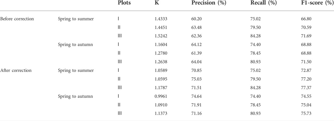
TABLE 4. Early warning assessment of S. alterniflora diffusion.
In addition to the influence of factors such as hay, there are also the following reasons, which will affect the spread prediction of S. alterniflora. Due to the subjective influence of people, there will be errors when drawing the contour boundary of S. alterniflora, resulting in errors when calculating the diffusion distance. Moreover, the spread of S. alterniflora is also affected by the surrounding environment. The speed of S. alterniflora spreading to tidal flats and mangroves is different. It is relatively easy to spread to tidal flats but relatively difficult to spread to mangroves. Therefore, there are limitations to diffusion prediction based on the average diffusion distance.
In this study, time-series UAV images were used to achieve accurate identification of S. alterniflora based on a CNN model, and a feasible method for early warning of S. alterniflora spread was proposed. To investigate the impact of different CNN models on S. alterniflora recognition, the spring dataset was used for training and evaluation. Through comparative analysis, ResNet50 is more suitable for the recognition of S. alterniflora; its precision on the test set is 97.61%, the recall is 95.22%, and the F1-score is 96.40%. To study the effect of different seasons on the accurate identification of S. alterniflora, ResNet50 was trained and evaluated using a combination of datasets in different seasons. The results show that the single-season model can better identify S. alterniflora in its own season, but it is difficult to accurately identify S. alterniflora in the whole year using only single-season data. The characteristics of S. alterniflora in winter are significantly different from those in other seasons, and it is difficult to accurately identify S. alterniflora in winter through datasets from other seasons. For the monitoring of S. alterniflora throughout the year, the autumn-winter two-season model was selected from the perspective of time cost, the four-season model was selected from the perspective of identification performance, and the three-season model of summer, autumn and winter was selected from the perspective of time cost and identification performance. In addition, the diffusion of S. alterniflora from spring to summer and spring to autumn was predicted. By comparing the actual and predicted distributions of S. alterniflora, its predictive performance was evaluated, and possible causes of errors were analysed. The results showed that the early warning of S. alterniflora reflected the actual spreading trend of S. alterniflora to a certain extent. Using this method to predict the future spread of S. alterniflora has certain feasibility.
The datasets presented in this study can be found in online repositories. The names of the repository/repositories and accession number(s) can be found below: The author uploaded all relevant codes and datasets to figshare (https://doi.org/10.6084/m9.figshare.20654589).
XQ and YL: methodology, software, validation, writing. FQ: methodology, software, investigation, validation, writing-original draft, writing-review. YH: software, data curation, investigation. BL and CL: project administration. XP and FW: project administration. WQ: project administration, writing-original draft, writing-review and editing. All authors contributed to the article and approved the submitted version.
The work in this paper was supported by the National Natural Science Foundation of China (32272633), the National Key Research and Development Program of China (2021YFD1400100, 2021YFD1400101), and the Guangxi Ba-Gui Scholars Program of China (2019A33).
The authors thank the native English-speaking experts from the editing team of American Journal Experts for polishing our paper.
The authors declare that the research was conducted in the absence of any commercial or financial relationships that could be construed as a potential conflict of interest.
All claims expressed in this article are solely those of the authors and do not necessarily represent those of their affiliated organizations, or those of the publisher, the editors and the reviewers. Any product that may be evaluated in this article, or claim that may be made by its manufacturer, is not guaranteed or endorsed by the publisher.
Abade, A., Ferreira, P. A., and de Barros Vidal, F. (2021). Plant diseases recognition on images using convolutional neural networks: A systematic review. Comput. Electron. Agric. 185, 106125. doi:10.1016/j.compag.2021.106125
Ai, J. Q., Gao, W., Gao, Z. Q., Shi, R. H., and Zhang, C. (2017). Phenology-based Spartina alterniflora mapping in coastal wetland of the Yangtze Estuary using time series of Gaofen satellite no. 1 wide field of view imagery. J. Appl. Remote Sens. 11, 026020. doi:10.1117/1.Jrs.11.026020
An, S. Q., Gu, B. H., Zhou, C. F., Wang, Z. S., Deng, Z. F., Zhi, Y. B., et al. (2007). Spartina invasion in China: Implications for invasive species management and future research. Weed Res. 47 (3), 183–191. doi:10.1111/j.1365-3180.2007.00559.x
Bradley, B. A. (2014). Remote detection of invasive plants: A review of spectral, textural and phenological approaches. Biol. Invasions 16 (7), 1411–1425. doi:10.1007/s10530-013-0578-9
Chen, M., Ke, Y., Bai, J., Li, P., Lyu, M., Gong, Z., et al. (2020). Monitoring early stage invasion of exotic Spartina alterniflora using deep-learning super-resolution techniques based on multisource high-resolution satellite imagery: A case study in the yellow river delta, China. Int. J. Appl. Earth Observation Geoinformation 92, 102180. doi:10.1016/j.jag.2020.102180
Chung, C.-H. (2006). Forty years of ecological engineering with Spartina plantations in China. Ecol. Eng. 27 (1), 49–57. doi:10.1016/j.ecoleng.2005.09.012
Cui, B. S., He, Q., and An, Y. (2011). Spartina alterniflora invasions and effects on crab communities in a Western Pacific estuary. Ecol. Eng. 37 (11), 1920–1924. doi:10.1016/j.ecoleng.2011.06.021
Grosse-Stoltenberg, A., Hellmann, C., Thiele, J., Werner, C., and Oldeland, J. (2018). Early detection of GPP-related regime shifts after plant invasion by integrating imaging spectroscopy with airborne LiDAR. Remote Sens. Environ. 209, 780–792. doi:10.1016/j.rse.2018.02.038
Hang, J., Zhang, D., Chen, P., Zhang, J., and Wang, B. (2019). Classification of plant leaf diseases based on improved convolutional neural network. Sensors 19 (19), 4161. doi:10.3390/s19194161
He, Y. X., Guan, W., Xue, D., Liu, L. F., Peng, C. H., Liao, B. W., et al. (2019). Comparison of methane emissions among invasive and native mangrove species in Dongzhaigang, Hainan Island. Sci. Total Environ. 697, 133945. doi:10.1016/j.scitotenv.2019.133945
Krizhevsky, A., Sutskever, I., and Hinton, G. (2012)“ImageNet classification with deep convolutional neural networks,” in NIPS).
Lawrence, R. L., Wood, S. D., and Sheley, R. L. (2006). Mapping invasive plants using hyperspectral imagery and Breiman Cutler classifications (RandomForest). Remote Sens. Environ. 100 (3), 356–362. doi:10.1016/j.rse.2005.10.014
Li, B., Liao, C. H., Zhang, X. D., Chen, H. L., Wang, Q., Chen, Z. Y., et al. (2009). Spartina alterniflora invasions in the Yangtze River estuary, China: An overview of current status and ecosystem effects. Ecol. Eng. 35 (4), 511–520. doi:10.1016/j.ecoleng.2008.05.013
Li, N., Li, L. W., Zhang, Y. L., and Wu, M. (2020). Monitoring of the invasion of Spartina alterniflora from 1985 to 2015 in zhejiang province, China. BMC Ecol. 20 (1), 7. doi:10.1186/s12898-020-00277-8
Liu, M. Y., Li, H. Y., Li, L., Man, W. D., Jia, M. M., Wang, Z. M., et al. (2017). Monitoring the invasion of Spartina alterniflora using multi-source high-resolution imagery in the zhangjiang estuary, China. Remote Sens. 9 (6), 539. doi:10.3390/rs9060539
Liu, M. Y., Mao, D. H., Wang, Z. M., Li, L., Man, W. D., Jia, M. M., et al. (2018). Rapid invasion of Spartina alterniflora in the coastal zone of mainland China: New observations from landsat OLI images. Remote Sens. 10 (12), 1933. doi:10.3390/rs10121933
Martin, F.-M., Mullerova, J., Borgniet, L., Dommanget, F., Breton, V., and Evette, A. (2018). Using single- and multi-date UAV and satellite imagery to accurately monitor invasive knotweed species. Remote Sens. 10 (10), 1662. doi:10.3390/rs10101662
O'Donnell, J. P. R., and Schalles, J. F. (2016). Examination of abiotic drivers and their influence on Spartina alterniflora biomass over a twenty-eight year period using landsat 5 TM satellite imagery of the Central Georgia coast. Remote Sens. 8 (6), 477. doi:10.3390/rs8060477
Ren, G. B., Wang, J. J., Wang, A. D., Wang, J. B., Zhu, Y. L., Wu, P. Q., et al. (2019). Monitoring the invasion of smooth cordgrass Spartina alterniflora within the modern yellow river delta using remote sensing. J. Coast. Res. 90, 135–145. doi:10.2112/si90-017.1
Ren, G., Liu, Y., Ma, Y., and Zhang, J. (2014). Spartina alterniflora monitoring and change analysis in yellow river delta by remote sensing technology. Acta Laser Biol. Sin. 23 (6), 596–603.
Simonyan, K., and Zisserman, A. (2014). Very deep convolutional networks for large-scale image recognition. Comput. Sci.
Szegedy, C., Liu, W., Jia, Y., Sermanet, P., Reed, S. E., Anguelov, D., et al. (2014). Going deeper with convolutions, 4842. CoRR abs/1409.
Tan, M. X., and Le, Q. V. (2019).“EfficientNet: Rethinking model scaling for convolutional neural networks,” in 36th International Conference on Machine Learning ICML (SAN DIEGO: Jmlr-Journal Machine Learning Research).
Tian, Y. L., Jia, M. M., Wang, Z. M., Mao, D. H., Du, B. J., and Wang, C. (2020). Monitoring invasion process of Spartina alterniflora by seasonal sentinel-2 imagery and an object-based random forest classification. Remote Sens. 12 (9), 1383. doi:10.3390/rs12091383
Vaz, A. S., Alcaraz-Segura, D., Campos, J. C., Vicente, J. R., and Honrado, J. P. (2018). Managing plant invasions through the lens of remote sensing: A review of progress and the way forward. Sci. Total Environ. 642, 1328–1339. doi:10.1016/j.scitotenv.2018.06.134
Wang, A., Chen, J., Jing, C., Ye, G., Wu, J., Huang, Z., et al. (2015). Monitoring the invasion of Spartina alterniflora from 1993 to 2014 with landsat TM and SPOT 6 satellite data in yueqing bay, China. Plos One 10 (8), e0135538. doi:10.1371/journal.pone.0135538
Wang, J. B., Lin, Z. Y., Ma, Y. Q., Ren, G. B., Xu, Z. J., Song, X. K., et al. (2021). Distribution and invasion of Spartina alterniflora within the Jiaozhou Bay monitored by remote sensing image. Acta Oceanol. Sin. 41, 31–40. doi:10.1007/s13131-021-1907-y
Wu, Y. Q., Xiao, X. M., Chen, R. Q., Ma, J., Wang, X. X., Zhang, Y. N., et al. (2020). Tracking the phenology and expansion of Spartina alterniflora coastal wetland by time series MODIS and Landsat images. Multimed. Tools Appl. 79 (7-8), 5175–5195. doi:10.1007/s11042-018-6314-9
Xu, R. L., Zhao, S. Q., and Ke, Y. H. (2021). A simple phenology-based vegetation index for mapping invasive Spartina alterniflora using google earth engine. IEEE J. Sel. Top. Appl. Earth Obs. Remote Sens. 14, 190–201. doi:10.1109/jstars.2020.3038648
Yang, R. M. (2020). Characterization of the salt marsh soils and visible-near-infrared spectroscopy along a chronosequence of Spartina alterniflora invasion in a coastal wetland of eastern China. Geoderma 362, 114138. doi:10.1016/j.geoderma.2019.114138
Zhang, X., Xiao, X. M., Wang, X. X., Xu, X., Chen, B. Q., Wang, J., et al. (2020). Quantifying expansion and removal of Spartina alterniflora on Chongming island, China, using time series Landsat images during 1995-2018. Remote Sens. Environ. 247, 111916. doi:10.1016/j.rse.2020.111916
Zhu, W. Q., Ren, G. B., Wang, J. P., Wang, J. B., Hu, Y. B., Lin, Z. Y., et al. (2022). Monitoring the invasive plant Spartina alterniflora in jiangsu coastal wetland using MRCNN and long-time series landsat data. Remote Sens. 14 (11), 2630. doi:10.3390/rs14112630
Zhu, X. D., Meng, L. X., Zhang, Y. H., Weng, Q. H., and Morris, J. (2019). Tidal and meteorological influences on the growth of invasive Spartina alterniflora: Evidence from UAV remote sensing. Remote Sens. 11 (10), 1208. doi:10.3390/rs11101208
Keywords: Spartina alterniflora, UAV, image analysis, invasive plant, deep learning
Citation: Li Y, Qin F, He Y, Liu B, Liu C, Pu X, Wan F, Qiao X and Qian W (2022) The effect of season on Spartina alterniflora identification and monitoring. Front. Environ. Sci. 10:1044839. doi: 10.3389/fenvs.2022.1044839
Received: 16 September 2022; Accepted: 11 October 2022;
Published: 21 October 2022.
Edited by:
Xudong Zhu, Xiamen University, ChinaReviewed by:
Xingwang Fan, Nanjing Institute of Geography and Limnology (CAS), ChinaCopyright © 2022 Li, Qin, He, Liu, Liu, Pu, Wan, Qiao and Qian. This is an open-access article distributed under the terms of the Creative Commons Attribution License (CC BY). The use, distribution or reproduction in other forums is permitted, provided the original author(s) and the copyright owner(s) are credited and that the original publication in this journal is cited, in accordance with accepted academic practice. No use, distribution or reproduction is permitted which does not comply with these terms.
*Correspondence: Wanqiang Qian, cWlhbndhbnFpYW5nQGNhYXMuY24=; Xi Qiao, cWlhb3hpQGNhYXMuY24=; Fanghao Wan, d2FuZmFuZ2hhb0BjYWFzLmNu
†These authors have contributed equally to this work
Disclaimer: All claims expressed in this article are solely those of the authors and do not necessarily represent those of their affiliated organizations, or those of the publisher, the editors and the reviewers. Any product that may be evaluated in this article or claim that may be made by its manufacturer is not guaranteed or endorsed by the publisher.
Research integrity at Frontiers
Learn more about the work of our research integrity team to safeguard the quality of each article we publish.