Spatiotemporal model based on transformer for bias correction and temporal downscaling of forecasts

Numerical weather prediction (NWP) provides the future state of the atmosphere and is a major tool for weather forecasting. However, NWP has inevitable errors and requires bias correction to obtain more accurate forecasts. NWP is based on discrete numerical calculations, which inevitably result in a loss in resolution, and downscaling provides important support for obtaining detailed weather forecasts. In this paper, based on the spatio-temporal modeling approach, the Spatio-Temporal Transformer U-Net (ST-UNet) is constructed based on the U-net framework using the swin transformer and convolution to perform bias correction and temporal downscaling. The encoder part extracts features from the multi-time forecasts, and the decoder part uses the features from the encoder part and the constructed query vector for feature reconstruction. Besides, the query builder block generates different query vectors to accomplish different tasks. Multi-time bias correction was conducted for the 2-m temperature and the 10-m wind component. The results showed that the deep learning model significantly outperformed the anomaly numerical correction with observations, and ST-UNet also outperformed the U-Net model for single-time bias correction and the 3-dimensional U-Net (3D-UNet) model for multi-time bias correction. Forecasts from ST-UNet obtained the smallest root mean square error and the largest accuracy and correlation coefficient on both the 2-m temperature and 10-m wind component experiments. Meanwhile, temporal downscaling was performed to obtain hourly forecasts based on ST-UNet, which increased the temporal resolution and reduced the root mean square error by 0.78 compared to the original forecasts. Therefore, our proposed model can be applied to both bias correction and temporal downscaling tasks and achieve good accuracy.

1 Introduction

Weather changes have a great impact on human life and production, and accurately learning about the future state of the weather is significant. Weather forecasting, as a method of predicting the future state of the atmosphere, has always been a fundamental issue and a research hotspot in the field of atmospheric science (Bauer et al., 2015). Nowadays, operational weather forecasting is based on NWP models, which use powerful computers to perform numerical calculations to solve the hydrodynamic and thermodynamic equations describing the evolution of weather, thus predicting the future state of atmospheric motion and weather phenomena (Bauer et al., 2015; Krishnamupti and Bounoua, 2018). Attributed to the development of computer technology (Shuman, 1989; Lapillonne et al., 2016), model technology (Kalnay et al., 1996) and observational tools (Schulze, 2007; Leuenberger et al., 2020), NWP has made great progress in the last few decades.

However, NWP still suffers from unavoidable errors and a deficiency in model resolution. The NWP model cannot accurately describe sub-grid processes, while the numerical calculation process is approximated and the initial field is inaccurate. As a result, there are errors in the NWP, which are divided into initial field errors and model errors (Privé and Errico, 2013). Data assimilation can be used to obtain a more realistic state of the atmosphere by fusing satellite, radar, and other observations, thus providing an accurate initial field (Ghil and Malanotte-Rizzoli, 1991). Ensemble forecasts, which make use of forecasts from different conditions to compensate for the model’s lack of description of physical processes and the uncertainty of other factors, have been used in practical applications (Zhu, 2005; Qiao et al., 2020). However, many industries such as agriculture and transportation require accurate weather forecasts, so NWP forecasts need further corrections. Meanwhile, due to the limitation of computational and storage resources, NWP forecasts are limited in spatial and temporal resolutions, which makes it difficult to provide finer spatial and temporal forecast results. To address this issue, downscaling methods have been developed.

For bias correction, many methods have been proposed, including model output statistics (MOS) (Glahn and Lowry, 1972), anomaly numerical correction with Observations (ANO) (Peng et al., 2013), Bayesian model averaging (BMA) (Sloughter et al., 2010), the Kalman filter (Yang, 2019), and model output machine learning (MOML) (Li et al., 2019). MOS uses multivariate linear equations to establish the relationship between observations and forecasts, which relies on a large amount of data. Based on the theory that atmospheric states can be divided into climate-averaged and perturbed states (Qian, 2012), ANO overlays the difference between the climate-averaged state of the observations and the climate-averaged state of the model to correct the model bias. However, during sudden weather changes, ANO is difficult to revise model outputs. BMA obtains the best forecasts by constructing probability density functions (PDFs), so it is strongly dependent on the accuracy of the PDFs. For MOML, a variety of machine learning algorithms such as the support vector machine and the random forest can be used to establish the relationship between multiple forecast elements and correction elements to realize bias correction (Cho et al., 2020), where the choice of forecast elements is important for MOML. The deep learning model can also be used for bias correction, which is described in the next paragraph. For downscaling problems, current research focuses on spatial downscaling, i.e., converting large-scale low-resolution model outputs into high-resolution data. Traditional downscaling methods include statistical downscaling and dynamical downscaling, which use statistical relationships and nested models, respectively. However, temporal downscaling is also important. A stochastic weather generator is applied to seasonal precipitation and temperature forecasts, which extends generalized linear modeling approach to stochastic weather generator and introduces the aggregated climate statistics as covariates (Kim et al., 2016). At present, less research studies in this field have applied deep learning methods.

With the rise of deep learning techniques, they have been widely used and have achieved great success in many fields, including atmospheric science (Wang et al., 2021). Deep learning has been applied to areas such as image classification and image segmentation, where the data is generally gridded and spatial feature extraction has greatly improved the capability of the models. In contrast, methods such as MOS, BMA, and MOML establish regression relationships for a single point, so deep learning has an advantage in extracting spatial features from forecast data. Meanwhile, deep learning models can be migrated to a wide range of tasks, and their parameters can be adjusted through training to achieve superior results. This also allows deep learning to accomplish many tasks in the field of atmospheric science, such as prediction, inversion, and bias correction. However, deep learning frameworks lack interpretability and are like black boxes. Therefore, constructing appropriate models for different tasks and adding physical meaning to the models is the direction of deep learning development. To realize precipitation nowcasting, models derived from the encoder-decoder framework are adopted to generate nowcasting by fusing radar data and satellite data (Shi et al., 2017; Zhang et al., 2021). To invert the meteorological elements such as precipitation, Wu et al. (2020a); Xue et al. (2021) constructed models based on the convolutional neural network (CNN) or recurrent neural network to achieve precipitation estimation by using satellite bright temperature data, topographic elevation data, and meteorological station data. Combining the discontinuity of precipitation and the ill-posed property of downscaling, a novel deep learning model was constructed by using the super-resolution reconstruction technique in deep learning to realize precipitation downscaling (Xiang et al., 2022). For bias correction, the UNet was used to conduct bias correction by combining multiple forecast elements of the model output (Chen et al., 2020; Han et al., 2021), which indicates that deep learning models can significantly reduce the error of the forecast data. Therefore, for bias correction and temporal downscaling, this paper attempts to propose a model based on deep learning method to complete the above tasks, and achieves better results than the previous methods.

In this study, the spatio-temporal transformer U-net (ST-UNet) is proposed based on spatio-temporal modeling to perform bias correction and temporal downscaling tasks. The shifted window (swin) transformer is a hierarchical structure based on the transformer, and it divides images into non-overlapping windows and shifted windows. The self-attention mechanism is applied to each of the non-overlapping windows and shifted windows to obtain global features. The traditional U-net model is also a hierarchical u-shaped structure based on CNN. This paper replaces CNN with the swin transformer to facilitate the local feature extraction of CNN. The bias correction and downscaling tasks are transformed into the image translation problem in deep learning, and the spatio-temporal information of forecasts is fully exploited. For meteorological elements, the atmospheric state at a given point and a given time is not only related to the surrounding atmosphere but also the atmospheric state before and after. That is, the atmosphere has a spatio-temporal evolution, so mining spatio-temporal features is conducive to bias correction, which is also an important basis for temporal downscaling. Based on spatio-temporal modeling, this paper uses multi-time forecasts as input while processing the spatio-temporal information. The encoder part processes the input to obtain different levels of features. The query builder block generates different query vectors for bias correction and downscaling tasks. The decoder uses the query vector and the features from the encoder to complete the feature reconstruction and generate the multi-time output. Finally, the capability of our proposed model for each of the two tasks was verified by bias correction on 2-m temperature and 10-m u component of wind and temporal downscaling on 2-m temperature.

2 Data description

In this study, bias correction and temporal downscaling are applied to the forecast data to obtain more accurate and detailed forecasts. The operational Global Forecast System forecast (GFS) data provided by the National Centers for Environmental Prediction is used in this study (National Centers for Environmental Prediction, National Weather Service, NOAA, U.S. Department of Commerce, 2015). GFS is 0.25° × 0.25° gridded data that includes a wide range of meteorological elements in the air and on the surface. The data has forecast time steps at a 3-h interval from 0 to 240 h and a 12-h interval from 240 to 384 h. The model forecast is performed at 00, 06, 12, and 18 UTC daily. As an alternative to ERA-Interim, ERA-5 is the fifth generation of the European Center for Medium-Range Weather Forecasts Reanalysis (ERA), which provides hourly estimates of atmospheric, terrestrial, and oceanic climate variables (Hersbach, 2016). ERA-5 uses advanced modeling and data assimilation systems to integrate historical observations and satellite data into global estimates, which can provide a more realistic state of the atmosphere (He et al., 2019; Hersbach et al., 2020). Thus, ERA-5 is as used the true data in this study. The ERA-5 data has the same spatial resolution as the GFS forecasts, but its temporal resolution is 1 h, so it provides a more detailed view of the atmospheric state.

Our research areas are 105°–120°E and 20°–40°N, which cover the central and eastern regions of China and have many different geographic features and weather conditions. The specific domain and geographic features are illustrated in Figure 1. For bias correction and temporal downscaling tasks, the multi-time data of GFS forecast is taken as input, and the ERA-5 data at the same moment provides the true atmospheric state as the output target.

FIGURE 1

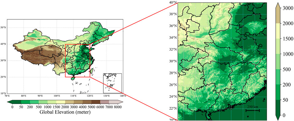
FIGURE 1. The study area. The colored bar represents the elevation of the terrain.

The GFS forecast data for the period from 15 January 2015 to 30 September 2020 is used in this study. For each forecast sample, the dataset is constructed by using the ERA-5 data corresponding to the forecast time as the true value. Meanwhile, to maintain the stability of the training process and to speed up the convergence, the raw data is normalized by using zero-mean normalization. The data from 15 January 2015 to 28 February 2019 is used as the training set, the data from 1 March 2019 to 31 August 2019 is used as the validation set, and the data from 1 September 2019 to 30 September 2020 is used as the test set. There are more than 8,000 samples in total. The ratio of training, validation, and test set is approximately 7:1:2.

3 Methods

Traditional bias correction methods make individual corrections to the forecast data at a given time. They cannot take full advantage of the temporal correlation of the forecast data and cost a lot of resources for repeated modeling (Han et al., 2021). Also, the elements of the atmosphere (e.g., temperature, humidity, wind field, etc.) are correlated in time. Therefore, it is more effective to perform bias correction on adjacent multi-time forecasts at a particular moment in time. Meanwhile, a multi-time bias correction model can be constructed, which uses multi-time forecasts as input to complete the bias correction of multi-time forecasts. Specifically, given the forecast result P at the issue time t₀ from the GFS, 3 days of forecasts are selected at an interval of 6 h, which is denoted as P′:

$P^{\prime }={\left\{P_{n,w\times h}^t\right\}}_{n=\mathrm{1,2},\dots ,Nw=\mathrm{1,2},\dots ,Wh=\mathrm{1,2},\dots ,H}^{t=t_0+1,t_0+2,\dots ,t_0+T}(1)$

where T denotes the length of the forecast time series, N denotes the number of meteorological elements, and W × H denotes the grid size of the forecast.

The ERA-5 data at the time corresponding to forecast data P′ is selected as the true value and denoted as G. For the bias correction or temporal downscaling task, the mapping relationship F between P′ and G need to be determined. Considering that the true state $G_{t_0}$ at the issue time t₀ is related to the forecast data P, it is also used as the input. Thus, for the bias correction task, we have the following equation:

$P_{\mathit{pre}}=F\left(P^{\prime },G_t\right)(2)$

where F denotes the mapping relationship for bias correction, and P_pre denotes the corrected forecast data.

The elements of the atmosphere are closely related and they evolve simultaneously in space and time. Also, temperature, relative humidity, and wind speed are closely related to each other (including the temporal and spatial distribution and error characteristics) in terms of the equation constraints of the NWP model and the dynamic, thermal, and micro-physical characteristics of the atmosphere. Therefore, other meteorological elements are introduced into the input. In this paper, 2-m temperature, 2-m relative humidity, and 10-m wind are used as inputs. Therefore, we have the following equation:

$P_{\mathit{pre}}=F\left(P_n^{\prime },G_t\right)(3)$

where $P_n^{\prime }$ represents the forecast data of n meteorological elements, including 2-m temperature, 2-m relative humidity, and 10-m wind.

In addition to the bias correction task, temporal downscaling is also performed, i.e., low-resolution forecast data are used in the time dimension to obtain high-resolution forecasts. Meanwhile, the same inputs are used, but forecasts are selected for 1 day at an interval of 3 h. Besides, hourly ERA-5 data in the same time range are used as true values. Then, by adapting the bias correction model, temporal downscaling results can be obtained. The whole process is described as follows:

$P_{\mathit{pre}}^{\prime }=F^{\prime }\left(P_n^{\prime },G_t\right)(4)$

where F′ represents the mapping relationship for temporal downscaling, and $P_{\mathit{pre}}^{\prime }$ denotes the forecast data after temporal downscaling.

In the following, the swin transformer and the specific framework of our proposed model will be introduced. Our model consists of three parts: the encoder, the decoder, and the query builder. The encoder uses the swin transformer for feature extraction and convolution for downsampling, and the above process is implemented in multiple layers. The query builder uses the features of the last layer in the encoder to generate the query vector. At different layers, the decoder combines the encoder’s feature processed by 3D convolution and the query vector to realize upsampling, and the final output is generated from the reconstructed features. By modifying the query builder, error correction and temporal downscaling can be accomplished. It is worth noting that different query vectors are constructed for different tasks, and the overall framework is shared.

3.1 Swin transformer

For gridded data such as images, CNN is applied for data processing (Khan et al., 2018). Because of its local and translation-invariant properties, the convolution operation is used in extracting spatial features from gridded data, and many network structures have been derived from CNN (Simonyan and Zisserman, 2014; Ronneberger et al., 2015). However, the receptive field of spatial extraction of CNN is limited. With the outstanding performance of the transformer in natural language processing, the transformer is gradually applied to computer vision for processing image data (Han et al., 2022). The core operation of the transformer is scaled dot-product attention (Vaswani et al., 2017). Given a query $Q\in {\mathbb{R}}^{n\times d_q}$ and a set of key-value pairs $K\in {\mathbb{R}}^{n\times d_q}$, $V\in {\mathbb{R}}^{n\times d_v}$, scaled dot-product attention calculates the attention score as:

$Attention\left(Q,K,V\right)=softmax\left(\frac{Q{K}^T}{\sqrt{d_k}}V\right)(5)$

where softmax is the softmax function, and $\frac{1}{\sqrt{d_k}}$ is the scaling factor.

To address the high computational consumption of the attention mechanism, many new versions have been proposed, such as informer, lite transformer, swin transformer (Wu et al., 2020b; Zhou et al., 2021a; Liu et al., 2021). The swin transformer uses a hierarchical structure and applies an attention mechanism to non-overlapping windows and shifted windows (Liu et al., 2021). It is an excellent transformer designed for computer vision applications and is used in our model to process spatio-temporal information from gridded forecasts.

3.2 Model

Based on the swin transformer and convolution, a spatio-temporal model is constructed in this study to perform the bias correction task and the temporal downscaling task, as shown in Figure 2. The spatio-temporal model based on the swin transformer has been designed and applied to video super-resolution tasks and action recognition tasks (Geng et al., 2022; Liu et al., 2022). The entire framework consists of an encoder, a decoder, and a query builder. The encoder extracts feature from the input, while the decoder used reconstructed features to generate the output. For the encoder and decoder, a series of swin transformers and convolution layers (including convolution and deconvolution) are used respectively. The swin transformer is used for feature extraction and reconstruction, while convolution and deconvolution are used for upsampling and downsampling, respectively. Features from different layers of the encoder are processed with 3-dimensional convolution and then used in the decoder. The query builder generates different initial queries and applies them to the decoder.

FIGURE 2

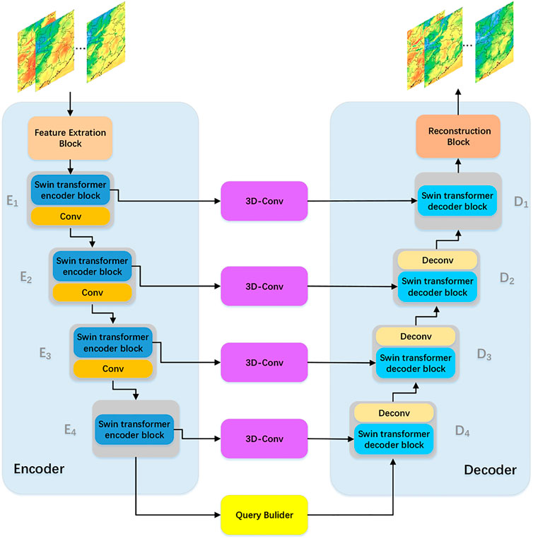
FIGURE 2. The overall structure of our proposes model.

3.2.1 Encoder

Firstly, the feature extraction block performs feature extraction on the input. The block consists of two-dimensional convolutions and normalization layers that map the input into higher dimensions. Then, the high-dimensional features are processed by a series of swin transformer encoder blocks, while each swin transformer encoder block is connected to a downsampling block consisting of a convolution (except for the last swin transformer). The downsampling block decreases the size of features by a factor of two, so different layers acquire information at different scales. The above is expressed as follows:

$\left\{\begin{array}{cc}{X}_k=T_{\mathit{swin}}\left(E_{k-1}\right),\hfill & k=\mathrm{1,2,3,4}\hfill \\ E_k=C_{\mathit{down}}\left(X_k\right),\hfill & k=\mathrm{1,2,3}\hfill \\ E_k=X_k,\hfill & k=4\hfill \end{array}\right.(6)$

where T_swin denotes the swin transformer encoder block, C_down denotes the downsampling block, X_k denotes the output of the swin transformer encoder block, and E_k denotes the output of each layer in the encoder.

As shown in Figure 3, the swin transformer encoder block consists of window-based multi-layer self-attention (W-MSA) and shifted window-based multi-layer self-attention (SW-MSA). The inputs are passed through a LayerNorm (LN) layer, the W-MSA, the LN, and a multi-layer perception (MLP) layer. The W-MSA lacks connections across windows, which limits its modeling power. Then, a shifted window partitioning approach called SW-MSA is proposed to introduce cross-window connections. The subsequent operations are consistent except for the change in the self-attention block.

FIGURE 3

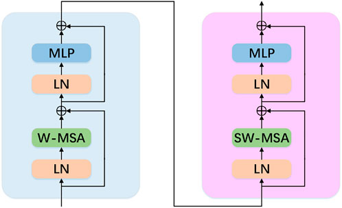
FIGURE 3. The structure of the swin transformer encoder block.

3.2.2 Query builder block

The output feature of each swin transformer encoder block has time steps of the same length, which is the same as the input. Only the size of the features is gradually reduced. The feature of the last block E_n is formulated as follows:

$E_n=\left(E_{n,3},E_{n,6},E_{n,9},\dots ,E_{n,3*T}\right)(7)$

where T represents the total length of the time steps of E_n, which remains the same as that of the input’s forecast time series.

To make the model suitable for different tasks, a query builder block is constructed. For the bias correction task, E_n is directly used as the initial query vector; for the time downscaling task, E_n is used to generate an initial query vector with a time series length consistent with the downscaling target. Thus, the following equation can be derived:

$Q=\left\{\begin{array}{cc}{E}_{n,t}\hfill & t=3k\hfill \\ \frac{2}{3}{E}_{n,t}+\frac{1}{3}{E}_{n,t+3}\hfill & t=3k+1\hfill \\ \frac{1}{3}{E}_{n,t}+\frac{2}{3}{E}_{n,t+3}\hfill & t=3k+2\hfill \end{array}\right.(8)$

where Q is the initial query vector. The above formula represents the initial query vector for temporal downscaling.

3.2.3 Decoder

In the decoder, multiple swin transformer decoder blocks and upsampling blocks are used. In each layer of the decoder, the swin transformer decoder block generates output features by the query vector acting on a dictionary of key-value pairs. Each swin transformer decoder block has two inputs: a feature from the encoder at the same layer, and a query vector. For the encoder’s features, 3-dimensional convolution is used to exploit the local feature extraction capability of convolution (Kopuklu et al., 2019). Unlike the 2-dimensional convolution, the 3-dimensional convolution can act on multiple dimensions in time and space to generate key-value pairs. The query vector is generated by the query builder block in the first layer and the output of the previous layer. Subsequently, the output of the swin transformer decoder block is upsampled by an upsampling block consisting of deconvolution. The whole process is shown below:

$\left\{\begin{array}{cc}{D}_k=C_{up}\left(T_{\mathit{swin}}\left(C_{3d}\left(X_k\right),Q\right)\right),\hfill & k=4\hfill \\ D_k=C_{up}\left(T_{\mathit{swin}}\left(C_{3d}\left(X_k\right),D_{k+1}\right)\right),\hfill & k=\mathrm{2,3}\hfill \\ D_k=T_{\mathit{swin}}\left(C_{3d}\left(X_k\right),D_{k+1}\right),\hfill & k=1\hfill \end{array}\right.(9)$

where T_swin denotes the swin transformer decoder block, C_up denotes the upsampling block, C_3d denotes the 3D convolution, and X_k denotes the output of the swin transformer encoder block.

The structure of the swin transformer decoder block is shown in Figure 4. The query vector is first passed through W-MSA. Then, the output feature from the encoder is used as a dictionary of key-value pairs, which passes through the window-based multi-layer cross-attention (W-MCA) with the query vector. The query vector acts on the dictionary of key-value pairs from the encoder to generate the features for the target task in W-MCA. The same operation is performed by SW-MSA and shifted window-based multi-layer cross-attention (SW-MCA). Finally, the feature from the final layer of the swin transformer decoder block is passed through the reconstruction block to generate the output. The reconstruction block consists of a series of residual blocks.

FIGURE 4

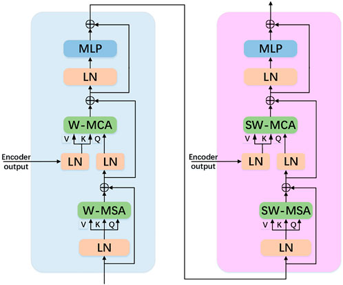
FIGURE 4. The structure of the swin transformer decoder block.

4 Experiment

4.1 Train details

The Adam optimizer with β1 = 0.9 and β2 = 0.999 is employed for training. The initial learning rate is set to 1 × e⁻⁴. Also, the learning rate exponential decay scheme is adopted to improve the stability of the training process, with the decay exponent parameter set to 0.98. The batch size is set to 8, and the loss function is set to the MSE loss function. Each model is trained for about 50 epochs. All models are implemented with PyTorch.

4.2 Baseline methods

Anomaly numerical correction with observations (ANO) is a traditional bias correction model that decomposes observations and model forecasts into climate mean state and disturbance state. The specific correction process of ANO is described as follows. The coordinate of a grid point is denoted as (i, j), and the climate mean state of forecasts p_i,j and the climate mean state of observations y_i,j are represented as:

$p_{i,j}=\frac{1}{N}\sum _{k=1}^N{p}_{i,j}(10)$

$y_{i,j}=\frac{1}{N}\sum _{k=1}^N{y}_{i,j}(11)$

Therefore, the corrected result is

$p_{i,j}^{\prime }=p_{i,j}-\left(p_{i,j}-y_{i,j}\right)(12)$

where $p_{i,j}^{\prime }$ is the corrected result, p_i,j represents the forecast result for grid point (i, j), y_i,j represents the observation data for grid point (i, j), and N represents the total number of samples. The forecasts are corrected for each forecast time separately. For more details of ANO, refer to (Peng et al., 2013).

The single-time correction model U-Net and the multi-time correction model 3D-UNet are taken for comparison to investigate the effectiveness of our proposed model against the classical deep learning-based bias correction model. The U-Net model is developed based on the encoder-decoder framework with two-dimensional convolution as the basic operation. It is commonly used in a variety of applications, such as image segmentation and image recognition (Ronneberger et al., 2015). Also, it has been used in bias correction, but only for single-time error revisions (Han et al., 2021). The 3D-UNet model replaces two-dimensional convolution with three-dimensional convolution, and it is also developed based on the encoder-decoder framework. It can handle temporal information, so it can be applied to multi-time bias correction (Chen et al., 2020). In the experiment, a version of 3D-UNet with an attention module is used as a baseline method (Oktay et al., 2018). For temporal downscaling, a video super-resolution model using 3-dimensional convolution and U-Net architecture is used as a baseline method (Kalluri et al., 2020), which models the temporal dynamics between the input frames to complete video frame interpolation. It can be used in temporal downscaling and we still name it as 3D-UNet. The parameters and training time of different models in detail is showed in Table 1.

TABLE 1

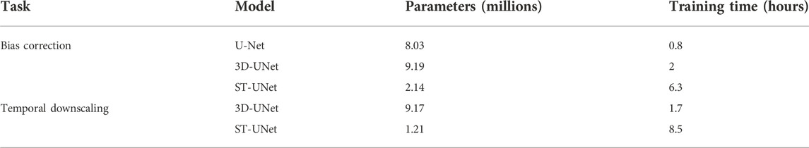
TABLE 1. The parameters and training time of different models in bias correction and temporal downscaling tasks.

4.3 Evaluation indicators

To evaluate the effectiveness of different methods for bias correction and temporal downscaling, mean absolute error (MAE), root mean square error (RMSE), correlation coefficient (CC), and accuracy (Acc) are employed as evaluation indicators. RMSE is a general metric for evaluating regression problems, and MAE can also be used to evaluate the error between the corrected and true values. CC characterizes the correlation degree between the corrected and true values, and Acc represents the accuracy of the corrected results. For the corrected or downscaled result P_pre, the corresponding true value is denoted as P_true. MAE and RMSE are calculated as:

$RMSE=\sqrt{\frac{1}{N}\sum _1^N{\frac{1}{T}\left({\mathbf{P}}_{\mathit{pre}}^n-{\mathbf{P}}_{\mathit{true}}^n\right)}^{\mathrm{2}}}(13)$

$MAE=\frac{1}{N}\sum _1^N\frac{1}{T}|{\mathbf{P}}_{\mathit{pre}}^n-{\mathbf{P}}_{\mathit{true}}^n|(14)$

$CC=\frac{\mathit{Cov}\left({\mathbf{P}}_{\mathit{pre}},{\mathbf{P}}_{\mathit{true}}\right)}{\sqrt{\mathit{Var}\left({\mathbf{P}}_{\mathit{pre}}\right)\mathit{Var}\left({\mathbf{P}}_{\mathit{true}}\right)}}(15)$

where P_pre represents the forecast result vector, P_true represents the true value vector, N represents the total number of samples, and T represents the total length of forecast time.

Accuracy is a metric that is often used for classification tasks. For regression tasks, the evaluation can be transformed into a binary classification problem by setting a threshold. If the threshold is set to σ, positive samples |P_pre − P_true| < σ are denoted as N_P, and negative samples |P_pre − P_true|≥ σ are denoted as N_G. Then the accuracy is expressed as:

$Acc=\frac{N_P}{N_G+N_P}\times 100\%(16)$

For various meteorological elements, the threshold σ has different values. According to (Chen et al., 2020), σ is set to 2°C to evaluate the post-processing methods of temperature forecasting. Accordingly, σ is set to 2 in our experiments of 2-m temperature. And σ is set to 1.5 in experiments for 10-m u component of wind.

It often happens that MAE, RMSE, CC, and Acc exhibit inconsistency in the experiments. For example, the value of RMSE decreases a lot, but the increase in Acc is not very significant. Here, a comprehensive statistic metric, DISO (the distance between indices of simulation and observation) is extended to evaluate the overall performance of different methods. If the statistical metrics for n chosen are (s¹, s², …, sⁿ) and the corresponding metrics between the truth data and itself are $(s_0^1,s_0^2,\dots ,s_0^n)$, then DISO is calculated as (Hu et al., 2019; Zhou et al., 2021b):

$DIS{O}_i=\sqrt{{\left(s_i^1-s_0^1\right)}^2+{\left(s_i^2-s_0^2\right)}^2+\cdots +{\left(s_i^n-s_0^n\right)}^2}(17)$

In this study, DISO, which is composed of four widely used statistical metrics: MAE, RMSE, CC, and Acc. In order to eliminate the influence of dimension, MAE and RMSE are normalized as Normalized MAE (NMAE) and Normalized RMSE (NRMSE) by dividing the maximum of MAE and RMSE respectively:

$DIS{O}_i=\sqrt{{\left(NMA{E}_i-NMA{E}_0\right)}^2+{\left(NRMS{E}_i-NRMS{E}_0\right)}^2+{\left(C{C}_i-C{C}_0\right)}^2+{\left(Ac{c}_i-Ac{c}_0\right)}^2}(18)$

If the result perfectly performs the best, the best statistical metrics are: NMAE = 0, NRMSE = 0, CC = 1, Acc = 1, then DISO can be expressed:

$DIS{O}_i=\sqrt{{\left(NMA{E}_i\right)}^2+{\left(NRMS{E}_i\right)}^2+{\left(C{C}_i-1\right)}^2+{\left(Ac{c}_i-1\right)}^2}(19)$

Now, the value of DISO expressed by the statistical metrics between the forecast and the truth are used to evaluate the performance of different methods. A larger value of DISO indicates that the method has a poorer performance.

5 Result

Our proposed model can perform both bias correction and temporal downscaling tasks, so it is evaluated in terms of the two tasks mentioned above on test set.

5.1 Bias correction

5.1.1 2-m temperature

Table 2 presents the overall effectiveness of different methods for the multi-time bias correction on 2 m temperature, while Table 3 presents the effectiveness of the bias correction on the 2-m temperature at the forecast time of 24 h. For the multi-time bias correction task, all methods show some improvement on the original GFS forecast data. Among them, the bias correction methods based on deep learning perform better than ANO. Compared with the 3D-UNet model based on convolution, our proposed model is based on the swin transformer. By utilizing the long-range information capture capability of the transformer structure, our proposed model achieves the best results. Meanwhile, the traditional U-Net model (Han et al., 2021) is taken to perform the bias correction of 24 h forecast to explore the effectiveness of the multi-time spatio-temporal correction method. It can be seen that the results based on spatio-temporal correction are significantly better than those of single-time correction, that is, 3D-UNet and ST-UNet are better than UNet. ST-UNet and 3D-UNet utilize not only the spatial distribution of the forecast data but also the temporal correlation of the forecast data, so they achieve better results, indicating that the spatio-temporal modeling approach has a better effect on bias correction. Besides, the ST-UNet based on the swin transformer obtains the best results for bias correction.

TABLE 2

TABLE 2. The overall performance of multi-time bias correction for the 2-m temperature on the test set.

TABLE 3

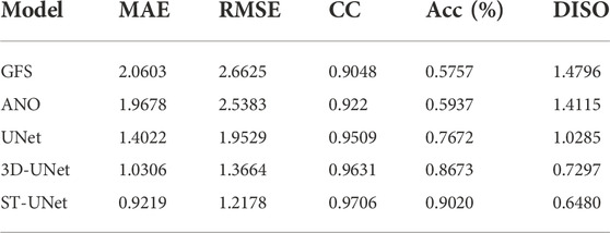
TABLE 3. The performance of bias correction for 2-m temperature of 24 h forecast on the test set.

To further demonstrate the multi-time bias correction of different methods, Figure 5 presents the RMSE of the corrected results for different forecast times. It can be seen that the RMSE of the forecasts increases with the forecast time, and the RMSE of GFS forecasts is always the highest. The ANO method provides some bias correction to the forecasts, but the results are still not satisfactory. Deep learning-based methods obtain good results. For our proposed ST-UNet, the RMSE is always the lowest, but the increase in RMSE with forecast time is also minimal, indicating that our model outperforms the CNN-based 3D-UNet model.

FIGURE 5

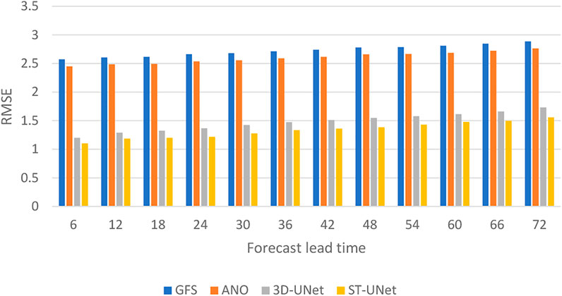
FIGURE 5. The RMSE of bias correction on the 2-m temperature for different forecast times on the test set.

To further investigate the effectiveness of different models, the RMSE spatial distribution of the bias correction results is plotted. Figure 6 shows the spatial distribution of RMSE for different methods, where (a), (b), (c), and (d) show the RMSE distributions in the same color range for different methods, and (e) and (f) show the RMSE distributions in the reduced color range for (c) and (d). From (a), (b), (c), and (d), it can be seen that the RMSE of ANO is reduced compared to that of the original GFS data, and the RMSE of the deep learning-based bias correction method is significantly reduced. This indicates the effectiveness of our spatio-temporal and multiple data fusion method and the obvious advantage of the deep learning model for bias correction. From (e) and (f), it can be observed that our proposed ST-UNet model outperforms the 3D-UNet model, as shown by the significant reduction of RMSE in the large value regions, especially in the central and northern parts of the study area.

FIGURE 6

FIGURE 6. The RMSE spatial distributions of bias correction for 2-m temperature on the test set over study area.

An example of bias correction is presented in Figure 7. Here, the results for the three forecast times of 24, 48, and 72 h are considered. It can be seen from the results that the ANO method only makes a simple correction to the original GFS, and the result is still quite different from the ERA-5 data. The 3D-UNet model and the ST-UNet model greatly improve the GFS data, and the results have similarities to the ERA-5 data in terms of spatial distribution. The ST-UNet model can obtain better results at the extremes and mutations than 3D-UNet, that is, and the spatial distribution of the data is more consistent with that of the ERA-5 data.

FIGURE 7

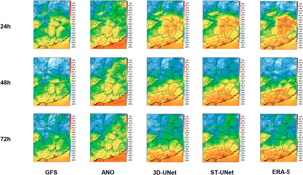
FIGURE 7. The distributions of 2-m temperature on the forecast time of 24, 48, and 72 h, including GFS, ERA-5, and corrected results from ANO, 3D-UNet, and ST-UNet.

5.1.2 10-m U component of wind

Experiments are also conducted on the 10-m u component of wind. Table 4 presents the overall effect of different methods on multi-time bias correction on the 10-m u component of wind. The results are similar to that of the 2-m temperature bias correction. Specifically, ANO has some improvements for GFS forecast data, and the method based on deep learning can greatly improve the GFS forecast data. Our proposed STUNet model performs the best with the smallest RMSE, MAE, and largest CC and Acc. Table 5 shows the effect of bias correction at the forecast time of 24 h. The methods based on spatio-temporal modeling still achieve better correction results than ANO. Meanwhile, Figure 8 shows the RMSE of the corrected results for different forecast times. Similar to the 2-m temperature bias correction, our proposed ST-UNet model always achieves the smallest RMSE as the forecast time increases.

TABLE 4

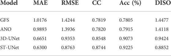
TABLE 4. The overall performance of multi-time bias correction for the 10-m u component of wind on the test set.

TABLE 5

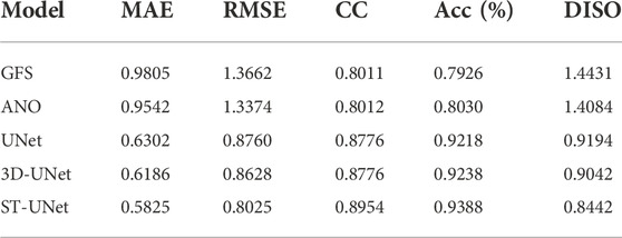
TABLE 5. The performance of bias correction for the 10-m u component of wind at the forecast time of 24 h on the test set.

FIGURE 8

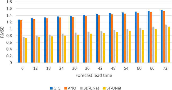
FIGURE 8. The RMSE of bias correction on the 10-m u component of wind for different forecast times on the test set.

Figure 9 presents the RMSE spatial distribution of bias correction, where (a), (b), (c), and (d) show the RMSE distributions in the same color range for different methods, and (e) and (f) show the RMSE distributions in the reduced color range for (c) and (d). 3D-UNet and ST-UNet largely reduce the RMSE across the study area, and the value of RMSE is much smaller than that of ANO. It can be seen from (e) and (f) that ST-UNet further reduces the RMSE in the region of extreme values, especially in the north of the study area.

FIGURE 9

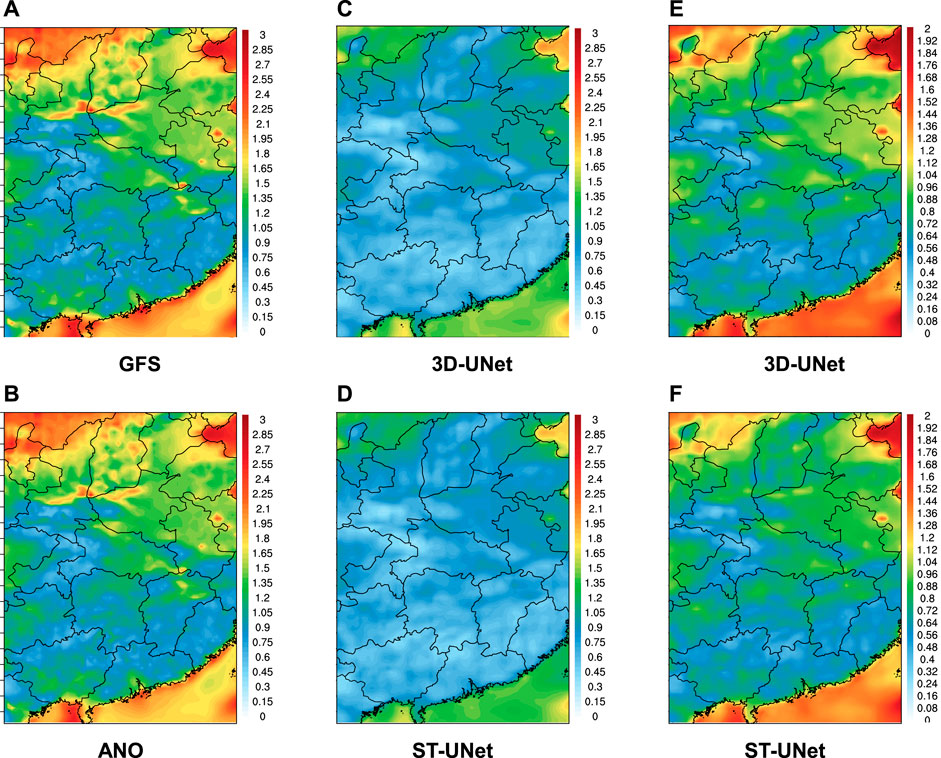
FIGURE 9. The RMSE spatial distribution of bias correction for the 10-m u component of wind on the test set over the study area.

5.2 Temporal downscaling

Due to the discretization of numerical calculations, forecast data products have resolution limitations. The temporal resolution of GFS forecast data is 3 h, and the GFS forecast data is downscaled. Using the ST-UNet model, the temporal resolution of the GFS forecast data is increased to 1 h. The whole temporal downscaling process improves the temporal resolution of forecast data. Meanwhile, since the same ground truth and model framework are used for bias correction, the whole downscaling process is accompanied by bias correction, so more accurate forecast data are also obtained. Therefore, the temporal downscaling process helps to obtain more detailed and precise forecast data.

A temporal downscaling experiment is conducted by using forecasts with a forecast time of 3 h–24 h at an interval of 3 h as input and the 2-m temperature of ERA-5 at an interval of 1 h as the true value. Similar to the bias correction, 2-m temperature, 2-m relative humidity, and 10-m wind are used as multi-element inputs, and the forecasts at an interval of 3 h would yield 2-m temperature results at an interval of 1 h. Table 6 presents the 2-m temperature temporal downscaling results. The RMSE of the GFS data is large, the RMSE of the downscaling results is significantly reduced, and the CC and Acc of the downscaling results are significantly increased. Figure 10 shows the RMSE of GFS and downscaling results over forecast time. It can be seen that our model still obtains a small RMSE for the downscaling results as the forecast time increases. Most importantly, for the missing forecast time, the RMSE of the downscaling results obtained by the ST-UNet model is still small and does not show abrupt increases, indicating that the proposed model is stable.

TABLE 6

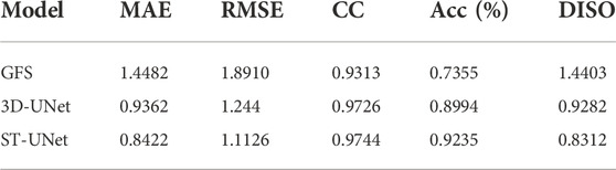
TABLE 6. The performance of temporal downscaling for 2-m temperature on the test set.

FIGURE 10

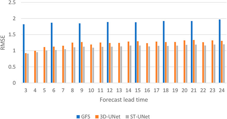
FIGURE 10. The RMSE of temporal downscaling on 2-m temperature for differents forecast times on the test set.

Figure 11 presents the results of a temporal downscaling example. The row “GFS” shows the forecast data of 18 h, 21 h, and 24 h; the rows of “ST-UNet” and “ERA-5” show the downscaling results and reanalysis data of 18–24 h, respectively. For the three forecast times of 18, 21, and 24 h, ST-UNet has a certain bias correction effect on the original GFS data; especially in the south of the study area, where the correction effect is obvious, and the area with large values is corrected. For other temporal downscaling results obtained by ST-UNet, they are consistent with the ERA5 data in the overall spatial distribution.

FIGURE 11

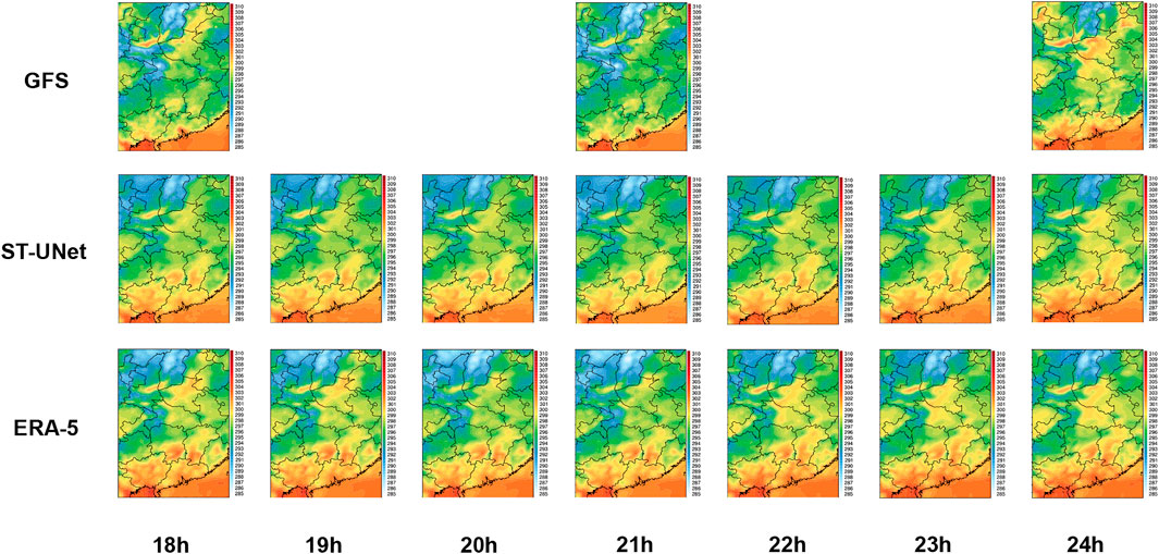
FIGURE 11. The distributions of 2-m temperature on the forecast time of 15–24 h, including GFS, ERA-5, and downscaling results obtained by ST-UNet.

6 Conclusion

In this paper, a deep learning model called ST-UNet is proposed based on spatio-temporal modeling to accomplish both bias correction and temporal downscaling. With the swin transformer as the main module and CNN as a supplement (Kopuklu et al., 2019; Liu et al., 2021), the ST-UNet model is constructed based on the framework of U-net. The encoder performs feature extraction and downsampling on the input, and the decoder applies the query vector to the features of the decoder to generate the output. To accomplish both the bias correction and downscaling tasks, a query builder block is proposed to generate the initial query vector. The main highlights of our work are as follows. Firstly, a spatio-temporal modeling approach that exploits both the spatial distribution and temporal correlation of forecast data is used, which performs better than single-time bias correction for the bias correction task; secondly, while previous work used CNNs for meteorological grid data, this paper uses the swin transformer, which exploits a self-attention mechanism to extract global features, thus achieving better results than 3D-UNet; thirdly, both the bias correction and temporal downscaling tasks are performed based on the ST-UNet model.

To verify the bias correction capability of our proposed model, multi-time bias correction of the 2-m temperature and the 10-m u component of wind is performed, and multiple types of multi-time forecasts are used as input. In the experiments, the deep learning model performs significantly better than ANO in bias correction, with a significant reduction in RMSE and a significant increase in CC and Acc. By analyzing the spatial distribution of RMSE, the deep learning approach can reduce RMSE significantly over the study range, while our proposed model obtains the smallest RMSE, especially in the regions with extreme values. To validate the temporal downscaling effect of our proposed model, temporal downscaling of 3-h forecasts is performed to obtain 1-h forecasts. In the 2-m temperature experiment, forecasts with errors much smaller than the original GFS are obtained, which indicates that the temporal downscaling process helps to obtain more detailed forecasts and correct the forecasts to obtain more accurate results.

In summary, our proposed model can perform both bias correction and spatial downscaling tasks to obtain more accurate and detailed forecast data. This process is based on spatio-temporal modeling and combines both the swin transformer module and the U-Net framework. Our proposed model can be applied to a wide range of model outputs and this will be the focus of our future research.

Data availability statement

The original contributions presented in the study are included in the article/Supplementary Material, further inquiries can be directed to the corresponding author.

Author contributions

LX and JG contributed to the conception and design of the study. LX organized the database. LX and JX performed the statistical analysis. LX wrote the first draft of the manuscript. LX, LZ, and FZ wrote sections of the manuscript. All authors contributed to the manuscript revision, and they read and approved the submitted version.

Funding

This work was supported by the National Natural Science Foundation of China (Grant No. 41975066).

Acknowledgments

We thank the reviewers for their comments, which helped us improve the manuscript.

Conflict of interest

The authors declare that the research was conducted in the absence of any commercial or financial relationships that could be construed as a potential conflict of interest.

Publisher’s note

All claims expressed in this article are solely those of the authors and do not necessarily represent those of their affiliated organizations, or those of the publisher, the editors and the reviewers. Any product that may be evaluated in this article, or claim that may be made by its manufacturer, is not guaranteed or endorsed by the publisher.

References

Bauer, P., Thorpe, A., and Brunet, G. (2015). The quiet revolution of numerical weather prediction. Nature 525, 47–55. doi:10.1038/nature14956

PubMed Abstract | CrossRef Full Text | Google Scholar

Chen, K., Wang, P., Yang, X., Zhang, N., and Wang, D. (2020). A model output deep learning method for grid temperature forecasts in tianjin area. Appl. Sci. 10, 5808. doi:10.3390/app10175808

CrossRef Full Text | Google Scholar

Cho, D., Yoo, C., Im, J., and Cha, D.-H. (2020). Comparative assessment of various machine learning-based bias correction methods for numerical weather prediction model forecasts of extreme air temperatures in urban areas. Earth Space Sci. 7, e2019EA000740. doi:10.1029/2019ea000740

CrossRef Full Text | Google Scholar

Geng, Z., Liang, L., Ding, T., and Zharkov, I. (2022). “Rstt: Real-time spatial temporal transformer for space-time video super-resolution,” in Proceedings of the IEEE/CVF Conference on Computer Vision and Pattern Recognition, 17441–17451.

CrossRef Full Text | Google Scholar

Ghil, M., and Malanotte-Rizzoli, P. (1991). Data assimilation in meteorology and oceanography. Adv. Geophys. 33, 141–266.

CrossRef Full Text | Google Scholar

Glahn, H. R., and Lowry, D. A. (1972). The use of model output statistics (mos) in objective weather forecasting. J. Appl. Meteor. 11, 1203–1211. doi:10.1175/1520-0450(1972)011<1203:tuomos>2.0.co;2

CrossRef Full Text | Google Scholar

Han, K., Wang, Y., Chen, H., Chen, X., Guo, J., Liu, Z., et al. (2022). A survey on vision transformer. IEEE Trans. pattern analysis Mach. Intell.

Google Scholar

Han, L., Chen, M., Chen, K., Chen, H., Zhang, Y., Lu, B., et al. (2021). A deep learning method for bias correction of ecmwf 24–240 h forecasts. Adv. Atmos. Sci. 38, 1444–1459. doi:10.1007/s00376-021-0215-y

CrossRef Full Text | Google Scholar

He, D., Zhou, Z., Kang, Z., and Liu, L. (2019). Numerical studies on forecast error correction of grapes model with variational approach. Adv. Meteorology 2019, 1–13. doi:10.1155/2019/2856289

CrossRef Full Text | Google Scholar

Hersbach, H., Bell, B., Berrisford, P., Hirahara, S., Horányi, A., Muñoz-Sabater, J., et al. (2020). The era5 global reanalysis. Q. J. R. Meteorol. Soc. 146, 1999–2049. doi:10.1002/qj.3803

CrossRef Full Text | Google Scholar

Hersbach, H. (2016). “The era5 atmospheric reanalysis,” in AGU fall meeting abstracts.

Google Scholar

Hu, Z., Chen, X., Zhou, Q., Chen, D., and Li, J. (2019). Diso: A rethink of Taylor diagram. Int. J. Climatol. 39, 2825–2832. doi:10.1002/joc.5972

CrossRef Full Text | Google Scholar

Kalluri, T., Pathak, D., Chandraker, M., and Tran, D. (2020). Flavr: Flow-agnostic video representations for fast frame interpolation [arXiv preprint arXiv:2012.08512].

Google Scholar

Kalnay, E., Kanamitsu, M., Kistler, R., Collins, W., Deaven, D., Gandin, L., et al. (1996). The ncep/ncar 40-year reanalysis project. Bull. Am. Meteorol. Soc. 77, 437–471. doi:10.1175/1520-0477(1996)077<0437:tnyrp>2.0.co;2

CrossRef Full Text | Google Scholar

Khan, S., Rahmani, H., Shah, S. A. A., and Bennamoun, M. (2018). A guide to convolutional neural networks for computer vision. Synthesis Lect. Comput. Vis. 8, 1–207. doi:10.2200/s00822ed1v01y201712cov015

CrossRef Full Text | Google Scholar

Kim, Y., Rajagopalan, B., and Lee, G. (2016). Temporal statistical downscaling of precipitation and temperature forecasts using a stochastic weather generator. Adv. Atmos. Sci. 33, 175–183. doi:10.1007/s00376-015-5115-6

CrossRef Full Text | Google Scholar

Kopuklu, O., Kose, N., Gunduz, A., and Rigoll, G. (2019). “Resource efficient 3d convolutional neural networks,” in Proceedings of the IEEE/CVF International Conference on Computer Vision Workshops.

CrossRef Full Text | Google Scholar

Krishnamupti, T., and Bounoua, L. (2018). An introduction to numerical weather prediction techniques. Florida, United States: CRC Press.

Google Scholar

Lapillonne, X., Fuhrer, O., Spörri, P., Osuna, C., Walser, A., Arteaga, A., et al. (2016). “Operational numerical weather prediction on a gpu-accelerated cluster supercomputer,” in EGU General Assembly Conference Abstracts.

Google Scholar

Leuenberger, D., Haefele, A., Omanovic, N., Fengler, M., Martucci, G., Calpini, B., et al. (2020). Improving high-impact numerical weather prediction with lidar and drone observations. Bull. Am. Meteorological Soc. 101, E1036–E1051. doi:10.1175/bams-d-19-0119.1

CrossRef Full Text | Google Scholar

Li, H., Yu, C., Xia, J., Wang, Y., Zhu, J., and Zhang, P. (2019). A model output machine learning method for grid temperature forecasts in the beijing area. Adv. Atmos. Sci. 36, 1156–1170. doi:10.1007/s00376-019-9023-z

CrossRef Full Text | Google Scholar

Liu, Z., Lin, Y., Cao, Y., Hu, H., Wei, Y., Zhang, Z., et al. (2021). “Swin transformer: Hierarchical vision transformer using shifted windows,” in Proceedings of the IEEE/CVF International Conference on Computer Vision, 10012–10022.

CrossRef Full Text | Google Scholar

Liu, Z., Ning, J., Cao, Y., Wei, Y., Zhang, Z., Lin, S., et al. (2022). “Video swin transformer,” in Proceedings of the IEEE/CVF Conference on Computer Vision and Pattern Recognition, 3202–3211.

CrossRef Full Text | Google Scholar

National Centers for Environmental Prediction, National Weather Service, NOAA, U.S. Department of Commerce (2015). Ncep gfs 0.25 degree global forecast grids historical archive.

Google Scholar

Oktay, O., Schlemper, J., Folgoc, L. L., Lee, M., Heinrich, M., Misawa, K., et al. (2018). Attention u-net: Learning where to look for the pancreas.

Google Scholar

Peng, X., Che, Y., and Chang, J. (2013). A novel approach to improve numerical weather prediction skills by using anomaly integration and historical data. J. Geophys. Res. Atmos. 118, 8814–8826. doi:10.1002/jgrd.50682

CrossRef Full Text | Google Scholar

Privé, N. C., and Errico, R. M. (2013). The role of model and initial condition error in numerical weather forecasting investigated with an observing system simulation experiment. Tellus A Dyn. Meteorology Oceanogr. 65, 21740. doi:10.3402/tellusa.v65i0.21740

CrossRef Full Text | Google Scholar

Qian, W.-H. (2012). How to improve the skills of weather and climate predictions? Chin. J. Geophys. 55, 1532–1540.

Google Scholar

Qiao, S., Zou, M., Cheung, H. N., Zhou, W., Li, Q., Feng, G., et al. (2020). Predictability of the wintertime 500 hpa geopotential height over ural-siberia in the ncep climate forecast system. Clim. Dyn. 54, 1591–1606. doi:10.1007/s00382-019-05074-8

CrossRef Full Text | Google Scholar

Ronneberger, O., Fischer, P., and Brox, T. (2015). “U-net: Convolutional networks for biomedical image segmentation,” in International Conference on Medical image computing and computer-assisted intervention, 234–241.

CrossRef Full Text | Google Scholar

Schulze, G. (2007). Atmospheric observations and numerical weather prediction: Saeon review. South Afr. J. Sci. 103, 318–323.

Google Scholar

Shi, X., Gao, Z., Lausen, L., Wang, H., Yeung, D.-Y., Wong, W.-k., et al. (2017). Deep learning for precipitation nowcasting: A benchmark and a new model. Adv. neural Inf. Process. Syst. 30.

PubMed Abstract | Google Scholar

Shuman, F. G. (1989). History of numerical weather prediction at the national meteorological center. Weather Forecast. 4, 286–296. doi:10.1175/1520-0434(1989)004<0286:honwpa>2.0.co;2

CrossRef Full Text | Google Scholar

Simonyan, K., and Zisserman, A. (2014). Very deep convolutional networks for large-scale image recognition.

Google Scholar

Sloughter, J. M., Gneiting, T., and Raftery, A. E. (2010). Probabilistic wind speed forecasting using ensembles and bayesian model averaging. J. Am. Stat. Assoc. 105, 25–35. doi:10.1198/jasa.2009.ap08615

CrossRef Full Text | Google Scholar

Vaswani, A., Shazeer, N., Parmar, N., Uszkoreit, J., Jones, L., Gomez, A. N., et al. (2017). Attention is all you need. Adv. neural Inf. Process. Syst. 30.

PubMed Abstract | Google Scholar

Wang, R., Wang, D., Qi, J., Wu, J., Liang, S., and Huang, Z. (2021). “Research situation and development trends of deep learning application in meteorology,” in International Conference on Artificial Intelligence and Security, 451–462.

CrossRef Full Text | Google Scholar

Wu, H., Yang, Q., Liu, J., and Wang, G. (2020a). A spatiotemporal deep fusion model for merging satellite and gauge precipitation in China. J. Hydrology 584, 124664. doi:10.1016/j.jhydrol.2020.124664

CrossRef Full Text | Google Scholar

Wu, Z., Liu, Z., Lin, J., Lin, Y., and Han, S. (2020b). Lite transformer with long-short range attention.

Google Scholar

Xiang, L., Xiang, J., Guan, J., Zhang, F., Zhao, Y., and Zhang, L. (2022). A novel reference-based and gradient-guided deep learning model for daily precipitation downscaling. Atmosphere 13, 511. doi:10.3390/atmos13040511

CrossRef Full Text | Google Scholar

Xue, M., Hang, R., Liu, Q., Yuan, X.-T., and Lu, X. (2021). Cnn-based near-real-time precipitation estimation from fengyun-2 satellite over xinjiang, China. Atmos. Res. 250, 105337. doi:10.1016/j.atmosres.2020.105337

CrossRef Full Text | Google Scholar

Yang, D. (2019). On post-processing day-ahead nwp forecasts using kalman filtering. Sol. Energy 182, 179–181. doi:10.1016/j.solener.2019.02.044

CrossRef Full Text | Google Scholar

Zhang, F., Wang, X., Guan, J., Wu, M., and Guo, L. (2021). Rn-Net: A deep learning approach to 0–2 hour rainfall nowcasting based on radar and automatic weather station data. Sensors 21, 1981. doi:10.3390/s21061981

PubMed Abstract | CrossRef Full Text | Google Scholar

Zhou, H., Zhang, S., Peng, J., Zhang, S., Li, J., Xiong, H., et al. (2021a). Informer: Beyond efficient transformer for long sequence time-series forecasting. Proc. AAAI Conf. Artif. Intell. 35, 11106–11115. doi:10.1609/aaai.v35i12.17325

CrossRef Full Text | Google Scholar

Zhou, Q., Chen, D., Hu, Z., and Chen, X. (2021b). Decompositions of Taylor diagram and diso performance criteria. Int. J. Climatol. 41, 5726–5732. doi:10.1002/joc.7149

CrossRef Full Text | Google Scholar

Zhu, Y. (2005). Ensemble forecast: A new approach to uncertainty and predictability. Adv. Atmos. Sci. 22, 781–788. doi:10.1007/bf02918678

CrossRef Full Text | Google Scholar