 Steven Rubinyi1,2*
 Jasper Verschuur1
 Ran Goldblatt3
 Johannes Gussenbauer4Alexander Kowarik4Jenny Mannix3
 Brad Bottoms3Jim Hall1
- 1Environmental Change Institute, University of Oxford, Oxford, United Kingdom
- 2Urban, Disaster Risk Management, Resilience and Land Global Practice, The World Bank, Washington, DC, United States
- 3New Light Technologies Inc, Washington, DC, United States
- 4Statistics Austria, Vienna, Austria
The impacts of natural disasters are often disproportionally borne by poor or otherwise marginalized groups. However, while disaster risk modelling studies have made progress in quantifying the exposure of populations, limited advances have been made in determining the socioeconomic characteristics of these exposed populations. Here, we generate synthetic structural and socioeconomic microdata for around 9.5 million persons for six districts in Bangladesh as vector points using a combination of spatial microsimulation techniques and dasymetric modelling. We overlay the dataset with satellite-derived flood extents of Cyclone Fani, affecting the region in 2019, quantifying the number of exposed households, their socioeconomic characteristics, and the exposure bias of certain household variables. We demonstrate how combining various modelling techniques could provide novel insights into the exposure of poor and vulnerable groups, which could help inform the emergency response after extreme events as well targeting adaptation options to those most in need of them.
Introduction
An increasingly large number of people are exposed to the impacts of natural hazards, such as floods, droughts, and cyclones (Jongman et al., 2012; Tanoue et al., 2016; Formetta and Feyen, 2019). For instance, while global urban settlements grew by 85% over the period 1985–2015, settlements exposed to flooding grew by 122 percent (Rentschler et al., 2022a). However, the vulnerabilities of those populations exposed to climate-related risks are not spatially homogenous. Using subnational poverty data, Rentschler et al. estimate that of the 1.47 billion people that are exposed to an extreme flood event (i.e. 1-in-100 years), around 10% live under the $1.9 poverty threshold and around 40% live below the $5.5 poverty threshold (Rentschler et al., 2022b). Poorer populations may suffer disproportionately from disasters for several reasons. First of all, poorer households are often forced to live in hazard-prone areas and hence suffer a “poverty exposure bias”, as has been identified for certain types of hazards (e.g. droughts and urban floods) (Winsemius et al., 2018). Second, poor households generally have a greater share of their total assets exposed to hazard events (e.g. agricultural, livestock) or poorer quality assets (e.g. low quality housing stock) (Alam and Collins, 2010; Hallegatte et al., 2020). For example, during the 2015 Nepal Earthquake, most damages were attributed to rural housing structures comprised of low-strength masonry (Lallemant et al., 2017). Similarly, surveys after the 2005 floods in Mumbai showed that poor households lost 75% of their assets, while non-poor households lost only 30% (Hallegatte et al., 2020). Third, poor or otherwise marginalized groups often have fewer resources to prepare for, and lower coping capacity (e.g. access to finance, savings, social safety nets) to respond to, and recover from, hazard impact (Hallegatte and Rozenberg, 2017). After the 2012 cyclone in Samoa, poorer households faced inequal access to remittances, therefore experiencing difficulties in recovering from the event (Le De et al., 2015).
Over the last decades, significant advances have been made in our understanding of the spatial distribution of populations and built-up areas, driven by new high-resolution exposure data such as WorldPop (Tatem, 2017), the Global Human Settlement Layer (GHSL) (Melchiorri et al., 2018), and the Global Urban Footprint (Esch et al., 2017). These types of datasets have underpinned high resolution national and global disaster risk analysis (Smith et al., 2019; Dullaart et al., 2021; Rentschler et al., 2022a). Despite advancements in modelling the exposure of people, understanding the vulnerability of populations remains a challenge for risk modelling. While studies have evaluated the exposure of vulnerable groups on a subnational level for specific countries (Bangalore et al., 2016; Marzi et al., 2019; Lee et al., 2021), extending these type of analysis to high resolution point or gridded datasets is limited not only due to lack of reliable frequent and granular socioeconomic and demographic data, but also due to privacy concerns regarding the release of granular socioeconomic data (i.e. microdata) (Arzberger et al., 2004). The root of the challenge is an inherent trade-off between maximizing the usefulness of the survey data, and safeguarding anonymity (Arzberger et al., 2004). Removing location information is a key objective of anonymization, making spatially focused research particularly difficult to pursue without some sort of workaround. Thus, our ability to quantify disparities of exposure and vulnerability to climate-related risks at a highly granular level has remained limited.
To overcome the challenge of having limited socioeconomic data on a granular level for geospatial analysis, several advancements in microsimulation techniques have taken place over the last decades, driven by increases in computational power, development of new algorithms, and the growing willingness of governments to release census microdata. Microsimulation techniques, such as Small Area Estimation (SAE) approaches, can be used to improve the resolution of aggregates available for comparison (Ghosh and Rao, 1994). Aggregate releases of survey data are often paired with microdata releases, which provide individual or household attributes for a percentage of households (typically up to 10 percent) within the aggregated geographic unit (Arzberger et al., 2004). For instance, the Integrated Public Use Microdata Series (IPUMS) put significant efforts to populate a database of individual-level microdata samples, including from international census records. Together, microdata can be applied to SAE methodologies for the downscaling of the aggregate data, with SAE methodologies typically falling under one of two categories: statistical SAE techniques or spatial microsimulation techniques.
Statistical SAE techniques match explanatory variables from the higher-level data set with those available from a separate data set in the smaller area of interest. In situations where official microdata directly taken from the census records are not released or where attributes not collected in the census are required, surveys collecting similar attributes can be used instead, or in connection with official microdata for the purposes of SAE. This can be exemplified through the Elbers, Lanjouw and Lanjouw (ELL) method of SAE to derive estimates of poverty rates, which require supplemental attributes related to welfare not typically collected in a national census, and has been successfully applied in Bangladesh (Elbers et al., 2003) and Brazil (Elbers et al., 2008).
While anonymized household and individual level releases of microdata can help provide a baseline for understanding the distribution of socioeconomic and demographic attributes collected within a geographical area, it may not provide much further detail into the spatial variance of those attributes within the spatial unit. As such, population synthesis, i.e. the generation of new anonymous microdata for an entire “synthetic population” (Rubin, 1993; Beckman et al., 1996), is increasingly applied to create plausible higher resolution population datasets, including their socioeconomic characteristics (Wheaton et al., 2009). Creating a dataset of synthetic populations through spatial microsimulation techniques requires the application of algorithms to extract information from various data sources to construct an entirely new dataset with the required attributes of households (Münnich and Schürle, 2003). Although each method for spatial microsimulation SAE differs in substantial ways, they all “fit” the microdata to the multidimensional aggregates and generate representative synthetic populations. The raw synthetic population data can be useful on its own or can be re-aggregated into the smaller area of interest. Over the years, synthetic socioeconomic attributes are increasingly used to evaluate the socioeconomic impact of policies and programs (Williamson et al., 2002; Barthelemy and Toint, 2013) or to support dynamic agent-based simulation in disaster risk management (Grinberger et al., 2017). Despite the potential of spatial microsimulation for geospatial analysis, two challenges remain. Regardless of which method for spatial microsimulation SAE is employed, the output remains spatially aggregated. On top of that, although some attempts have been made to calculate uncertainty using certain spatial microsimulation techniques, the limited ability to explicitly capture model uncertainty remains a methodological weakness of the technique when used for SAE (Whitworth et al., 2017).
While SAE focuses on downscaling individual or household attributes, spatial population modelling focuses on the spatial distribution of individuals or households over a population surface. The primary difference between the two is that spatial population modelling focuses solely on the geographic distribution of the population over a discrete surface, while SAE techniques focus on the downscaling of socioeconomic attributes to a higher spatial resolution. As a result, both techniques rely heavily on the disaggregation of census data but approach it from a different perspective. Dasymetric modelling, a branch of areal interpolation, is often employed for spatial disaggregation of population data (Wright, 1936; Lam, 1983; Goodchild et al., 1993). The increasing availability of high-resolution Earth observation data (e.g. data collected by Sentinel and Landsat satellites) together with improvements in post-processing and analytical techniques have led to increasingly accurate dasymetric population modelling approaches, even up to global scales. Examples are the Gridded Population of the World Layer (currently GPWv4), which provides 1-km resolution population estimates (Doxsey-Whitfield et al., 2015), the High-Resolution Settlement Layer (HRSL), providing population estimates at 30 m resolution (Tiecke et al., 2017), and the WorldPop 100-m population dataset (Stevens et al., 2015; Tatem, 2017). A small number of studies have complemented dasymetric approaches with geospatial techniques to generate spatially referenced synthetic populations. For instance, RTI, an independent, non-profit research institute, has produced a synthetic household population database for 116 million households and 300 million individuals in the United States (Wheaton et al., 2009). Thomson et al. first used DHS data with dasymetric modelling techniques, using 19 covariate layers, to create a 100-m resolution probability layer of seven distinct household types (e.g. urban rich, rural poor) in Namibia (Thomson et al., 2018). Synthetic household points were derived from multinomial logistic regression computed in the R package SimPop and assigned to household locations as observed in high resolution satellite imagery (30 cm resolution). Hence, simulating close-to-reality geospatial household survey information across large regions in areas with otherwise limited household survey information held considerable promise to advance geospatial analyses that rely on detailed household survey data while maintaining the anonymity of households.
Altogether, the increasing availability of remotely sensed imagery and socioeconomic datasets, and the improvement in computational power and analytical approaches, have the potential to bridge the spatial mismatch between exposure and socioeconomic information. This could be particularly useful for disaster risk modelling and adaptation, not only to better quantify whether certain social groups are particularly exposed to hazard impacts, but also to target adaptation interventions to those that need it the most (Verschuur et al., 2020). However, to date, such microsimulation and population synthesis techniques have not yet been applied in high-resolution disaster risk modelling studies. As such, there is limited understanding how such approaches can improve disaster risk assessment and support investment planning of adaptation strategies.
In this study, we generate synthetic structural and socioeconomic microdata for six districts in coastal Bangladesh (around 9.5 million persons, comprising 2.2 million households). We use this dataset in combination flood inundation maps of Cyclone Fani (May 2019) derived from Sentinel-1 images to provide insight into the absolute exposure of households to flooding, as well as the relative exposure of potentially vulnerable households (i.e. the “exposure bias” of exposed versus non-exposed populations) within the study area. For each exposed household, we compare five socioeconomic indicators: type of housing material; toilet type; water source; access to electricity; and whether it is in an urban or rural area. We estimate the spatial heterogeneities of socioeconomically disadvantaged households across affected districts, as well as the exposure bias for each socioeconomic indicator. In the Supplementary Materials, we compare our results with those reported in the Cyclone Fani Joint Situation Analysis (NAWG, 2019). The methodology we propose relies entirely on publicly available information, and hence can be applied in other developing countries to provide more spatially nuanced insights into the vulnerability of populations to natural hazards. This type of information could enable decision-makers to better understand who is exposed to climate-related risks and help better target interventions that could benefit the poor or most vulnerable.
Methodology
In this study, we propose a methodology that combines spatial microsimulation techniques for generating synthetic populations together with dasymetric modelling to produce a dataset of spatially referenced synthetic households as point locations (hereafter referred to as synthetic household survey data, or SHSD). The methodology to create the SHSD entails three discrete steps: 1) generation of synthetic households inclusive of selected attributes to the lowest reasonable level of aggregation; 2) spatial disaggregation of household units using dasymetric modelling techniques; and, 3) pairing of synthetic households with location of household units based on the population distribution identified in the dasymetric model. This methodology is then applied to simulate the location and characteristics of 2.2 million households across six districts in the Bangladesh Coastal Zone (BCZ).
To demonstrate the potential of SHSD to augment disaster-related decision-making, policies, and investment planning, we examine the impacts of Cyclone Fani, which hit Bangladesh in 2019, on the population residing in the western part of the BCZ. To do this, we perform the following three steps: 1) develop a granular estimation of flood delineation to enhance our understanding of Cyclone Fani’s extent; 2) spatially overlay the flood extent with the SHSD; and, 3) analyze the socioeconomic characteristics of exposed households and compare the relative vulnerabilities of exposed and non-exposed households (‘exposure bias’).
Case study Bangladesh
The BCZ (47,201 km2) covers 19 districts and was home to approximately 37.2 million in 2011 (Bangladesh Bureau of Statistics, 2012) and 43.8 million at present (Bangladesh Bureau of Statistics, 2022). We focus on six districts in the western part of the Bangladesh Coastal Zone (BCZ); Bagerhat, Barguna, Khulna, Patuakhali, Pirojpur, and Satkhira (Figure 1). The area we examine in this study spans nearly 16,000 km2 and in 2011 was home to approximately 9.5 million people residing in 2.2 million households (Bangladesh Bureau of Statistics, 2012).
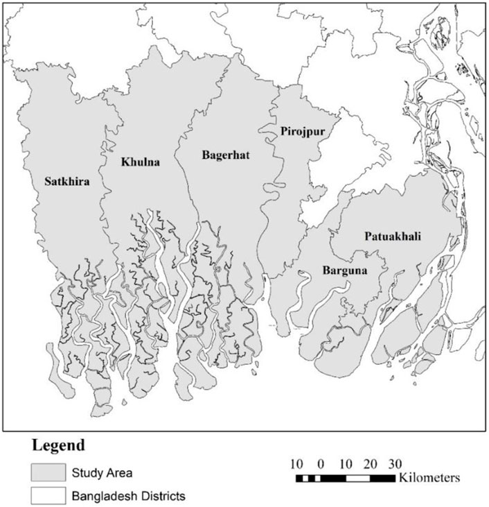
FIGURE 1. Study area comprised of (west to east) Satkhira, Khulna, Bagerhat, Pirojpur, Barguna, and Patuakhali districts.
The BCZ lags behind other parts of the country in socioeconomic development and struggles to cope with natural disasters and the gradual deterioration of the environment (Adams et al., 2016; Hossain et al., 2016). Existing challenges in the BCZ are likely to be exacerbated by the effects of climate change and associated sea-level rise (Dasgupta et al., 2010), with 62 percent of coastal lands being less than 3 m above sea level. The BCZ is highly vulnerable to tropical cyclones and subsequent storm surges, which are projected to increase in frequency and intensity in Bangladesh due to climate change (Dasgupta et al., 2010, 2014).
Creating the synthetic household survey data
We develop a methodology to simulate synthetic household locations. For each household we estimate its unique location (x and y coordinates) and a set of socioeconomic characteristics. To do this, we rely on the aggregate tables of the 2011 Bangladesh National Census at the union council level (admin level 4) (henceforth Census) (Bangladesh Bureau of Statistics, 2012), which are spatially disaggregated to point locations.
We derive the population synthesis using the framework provided by the R package simPop (Templ et al., 2017), an open-source and flexible synthesizer based on a modular object-oriented concept. This framework relies on aggregate tables for population margins and a microdata sample (both ideally from a population census), with the microdata sample containing at least all variables available in the aggregated tables. The steps for generating the synthetic population can be summarized as follows; 1) calibrate survey weights in the microdata to fit population margins, 2) extrapolate the microdata using alias sampling to generate the synthetic population, 3) set the variables of interest, household or personal variables, based on the microdata and “predict” them for each person in the synthetic population, and 4) use simulated annealing (SA) to calibrate the synthetic population to known population margins. The Supplementary Materials describes the detailed simulation and calibration procedure for creating the SHSD, while here we provide a brief overview of the methodology and how it is applied to the Census data.
Creating a target point layer
First, we convert the 2011 unconstrained WorldPop dataset for Bangladesh (∼100-m resolution) (WorldPop, 2017) from population counts (a float number) to household counts (an integer). The methodology to create WorldPop population density estimates considers spatial covariates such as nighttime lights, slope, elevation, and distance to features of both the built environment (e.g. urban areas, major road intersections) and the natural environment (e.g. inland waterbodies, sparsely vegetated areas) (Stevens et al., 2015).
For each union council (admin level 4), the average household size is calculated from Census data and spatially joined to the WorldPop layer. The WorldPop float population counts are then divided by the average household size within the union council, resulting in per-pixel household counts. To move from a polygon grid to a point layer, we create a dataset of randomly generated points within each cell corresponding to the integer value of households per cell. The point layer (representing locations of households) is spatially joined with the administrative boundaries (extracted from the Census) to associate a unique ID to each point. Figure 2 depicts approximately 58,000 predicted household point features across 550 km2 spanning Patharghata, Barguna Sadar, and Amtali upazilas in Barguna District, clearly depicting population clustering in densely populated areas.
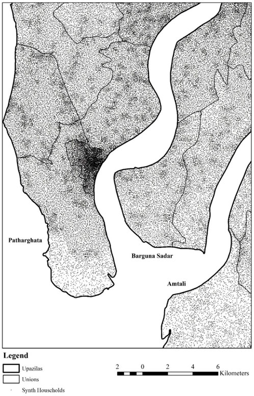
FIGURE 2. Point feature class of predicted household locations spanning Patharghata, Barguna Sadar, and Amtali upazilas in Barguna District.
Generating synthetic socioeconomic attributes
We generate synthetic structural and socioeconomic microdata for each of the 9.5 million persons grouped into 2.2 million households. Using the R package SimPop, the synthetic population is first generated to correspond with population margins for each union council. Then, each synthetic household is paired randomly with the derived target household point layer from the same union council. We rely on the following input data:
• Integrated Public Use Microdata Series (IPUMS): 5% sample microdata from the 2011 Bangladesh National Census includes topology at the upazila level (admin level 3).
• Census Tables: Aggregate tables from the 2011 Bangladesh National Census at the union council level (admin level 4).
• Demographic and Health Survey (DHS) Standard Data Set: 2011 DHS data set for Bangladesh.
We use variables from the sample microdata at the upazila level to generate a synthetic dataset at the union council level which is then matched to the aggregate Census tables. The DHS data is used to correct for age heaping as well as an underrepresentation of infants (see Supplementary Materials for details). For calibration, we used the maximum number of matching variables from the census tables to which we had access for this study.
The synthetic data contains three types of information (see Table 1). “Basic structural information” (sex, age, relationship to household head, urban/rural, upazila), which are created for each household and household member, are sampled from the microdata and are kept fixed to generate a realistic base. “Household-level variables” (housing type, housing structure, tenancy status, water source, electricity, sanitation) are defined on a household level and are modelled and appended to the “Basic structural variables”. “Individual-level variables” (years of schooling, literacy, level of education, employment status and industry) are modelled on an individual level and are appended to the “Basic structural variables”; and the “Household-level variables”. The steps for modelling these synthetic variables are described in more detail in Supplementary Materials.
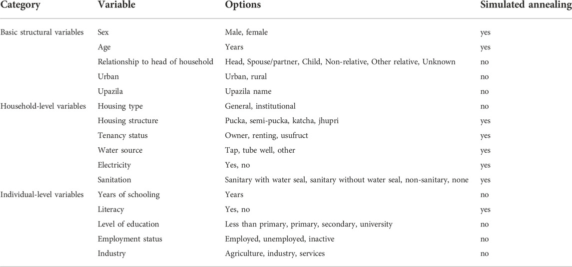
TABLE 1. Overview of the different variables in the synthetic dataset, including which variables are used in the calibration process using simulated annealing.
Calibrating the synthetic population
Initially, generated households are randomly assigned to union councils (admin level 4) within each upazila (admin level 3), matching the total number of households listed per union council in the Census tables. To achieve a more accurate distribution of households with certain properties at the union council level, we perform calibration through simulated annealing (SA). SA is the heuristic procedure used to approximate complex optimization problems (Templ et al., 2017), and has shown to outperform other methods, including deterministic re-weighting and conditional probabilities (Harland et al., 2012). We use the aggregate Census data at the union council level to estimate several household attributes (housing type, tenancy status, water source, electricity and sanitation) and individual attributes (sex, age, literacy) to better represent their distribution (and households overall) at the union council level (the calibration process is described in the Supplementary Materials).
Joining the synthetic population to the target point layer
Each point is randomly joined with a discrete synthetic household within the union council. This results in a household point feature that now contains the synthetic structural and socioeconomic attributes for each household as well as for all individual persons within a household.
Validation synthetic household survey data
To externally validate the SHSD generated, we collected an independent household survey dataset that covers three union councils in Khulna district. This dataset was collected as part of the REACH project, a global research program aimed at improving water security for the poor, and includes household attributes for 707 households (3,124 persons) in these three union councils (5.6% of population) during the period 17-12-2017 to 01-07-2018. We compare the age distribution, the only comparable household parameter in both survey data, and geographical locations between the REACH survey and almost 12,700 synthetic households that are sampled for these three unions councils. As shown in the Supplementary Materials, the field data corresponds to the SHSD in terms of age distribution (though slightly skewed towards a younger population). In terms of spatial correlation, 98% of all surveyed households are within 100 m of at least one synthetic one, with the median distance being 18 m.
Flood inundation associated with Cyclone Fani
We analyze the flood inundation associated with Cyclone Fani, which made landfall near Puri, India (03-05–2019) as a Category four tropical cyclone and proceeded in a northeasterly direction, eventually making landfall in Bangladesh (04-05–2019) by which time it had weakened into a deep depression. Cyclone Fani caused widespread inundation across 28 districts, inundating 60 villages, with the largest inundation in the six districts in our study area. In total, 1.6 million people were evacuated to cyclone shelters, 155,000 acres of agricultural land was affected and around 20,000 houses were damaged (NAWG, 2019).
Satellite remote sensing has emerged as a viable alternative or supplement to in situ hydrological observations especially over ungauged regions (Khan et al., 2011). In this study, we utilize Synthetic Aperture Radar (SAR) data collected by Sentinel-1 satellites. This constellation provides dual polarization capabilities, short revisit times and rapid product delivery using four C-band imaging modes with different resolutions (down to 5 m) and coverage (up to 400 km). Data collected by SAR sensors is especially useful for flood detection, due to the ability of these sensor to capture Earth at day and night, in all weather conditions (Chini et al., 2019; Malmgren-Hansen et al., 2020). The method of detecting inundated flood extents with SAR data relies on differences in the backscattered signal between surfaces that are covered and not covered with water. SAR data, including Sentinel-1 measurements, have shown to be effective in delineating floods, including in urban populated areas (Chini et al., 2019; Malmgren-Hansen et al., 2020).
To delineate potential flooded areas in the six Fani-affected districts, we apply an image differencing technique, where SAR images collected during a non-flooded state are compared against images collected during (or just after) the flood. Compared to flood detection with a single image, image differencing techniques are advantageous because they allow to mask out permanent water bodies and some water look-alike objects (Li et al., 2018). Satellite images can be mosaiced together to better capture the full extent of dynamic flood events. However, the full extent of flooding may be underestimated when the frequency of data capture is limited. We perform the analysis in Google Earth Engine (GEE), which has been previously used for flood detection and surface water mapping applications (Markert et al., 2018; Uddin et al., 2019).
To create the flood inundation maps, several processing steps are followed (the methodology is described in detail in the Supplementary Materials). First, we mosaic several Sentinel-1 scenes together before (28 April 2019) and after the event (4 May 2019). These are hereafter named the Base Image (BI) and the Event Image (EI). Sentinel-1 image has one or two out of four possible polarization bands. Here we use a single co-polarization, vertical transmit/vertical receive data (VV), which has a slight advantage over other polarization modes (Twele et al., 2016; Clement et al., 2018) and has successfully been used for flood mapping in previous studies (Schlaffer et al., 2015). Second, we remove permanent water bodies from the images, which may distort the flood inundation extent, and are taken from the Joint Research Center (JRC) Yearly Water Classification History dataset (version 1.1) (Pekel et al., 2016). Third, we create the Difference Image (DI) by subtracting the pixel values of the EI with the BI per grid cell. Fourth, to reduce the “noise” in the data, we smooth the DI by calculating a morphological reducer over the pixels in the image. The result of this step is a Smoothed Difference Image (SDI) which contains fewer isolated pixels that could potentially be misclassified in the subsequent steps. The final step in the analysis involves the conversion of the SDI into a binary map of observed flooded areas. We apply a thresholding technique that relies on the relative values (a percentile value) of the pixels in the study area, ending up with a binary flood inundation map of the study area at 10-m resolution.
Results
Flood inundation
Our flood mapping methodology generated 578 km2 of observed flooded areas (i.e. about 3.8 percent of the study area) with a widespread partial inundation across the study area, and several more concentrated clusters. Only six out of the 49 populated upazilas show more than 10 percent of their area flooded (Table 2). At a more granular level, five out of 436 union councils show more than 20 percent of their area flooded.
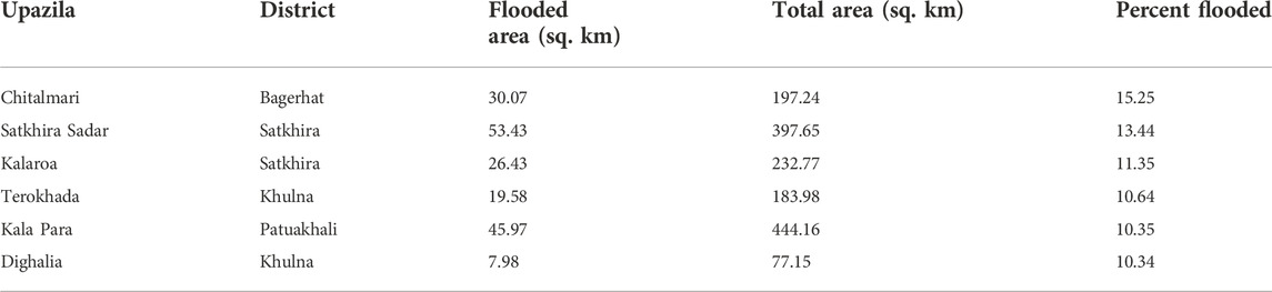
TABLE 2. Upazilas with at least 10 percent observed flooded area.
Overlaying the SHSD with the derived flood map results in a total of 105,116 households being exposed to flood inundation. Figure 3 provides a visual snapshot of a small section of the study area–depicting approximately 172,000 synthetic households across 780 km2 of Bagerhat and Pirojpur Districts. Nearly 46.3 km2 of land is predicted to be potentially flooded (highlighted in blue in the figure), within which reside approximately 6,000 households. Across the six districts, we observe a relatively equal share of households being flooded, with the highest percentage in Sathkira (∼5.5%) and Pirojpur (∼3.8%) districts, and lowest in Bagerhat, Barguna and Khulna districts (all ∼3%).
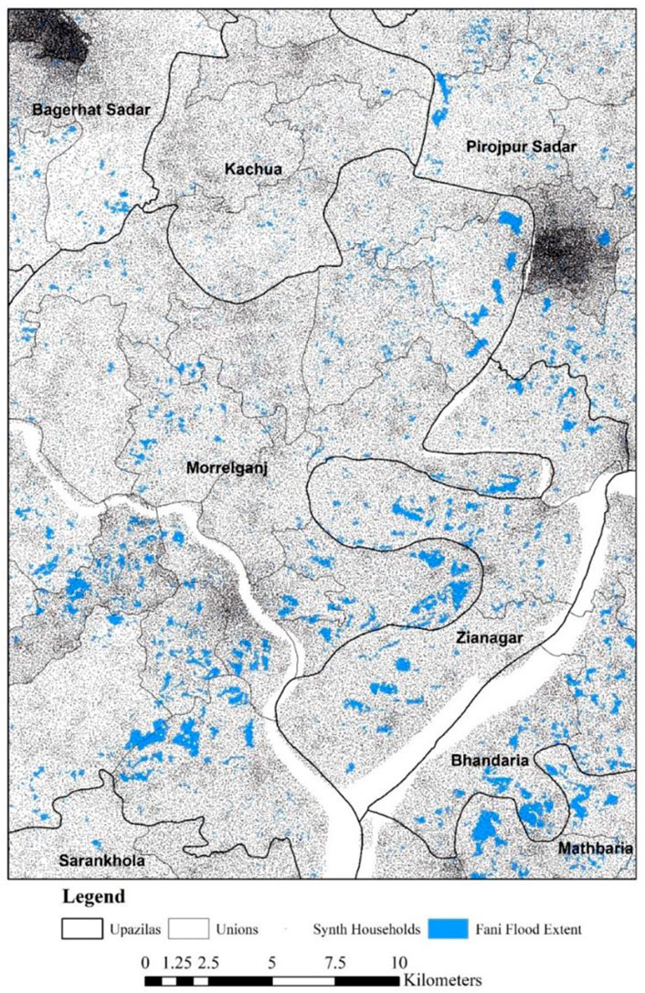
FIGURE 3. Synthetic households (dark points) and Cyclone Fani flood extent (in blue) spanning sections of Bagerhat and Pirojpur Districts.
Social vulnerability
Next, we take a closer look at the socioeconomic characteristics of potentially flooded households. Figure 4 provides a summary of selected socioeconomic characteristics from our 105,116 modelled flooded households, including: the type of housing material; toilet type; water source; access to electricity; and whether it resides in an urban or rural area. The left figures show the absolute count, while the right-hand side shows the relative share per district. The proportional distribution of modelled attributes by district provides a proxy for understanding the relative vulnerability of exposed households. For example, certain housing types are often associated with poorer households, such as jhupri and katcha structures (unimproved housing), while certain structure designs may also be better suited to withstand flooding than others (Dasgupta et al., 2010). Hence, households in jhupri structures are often poorer and are more likely to lose their house when being exposed to the same flood severity.
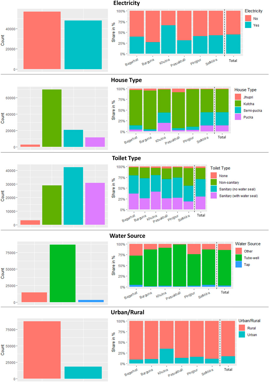
FIGURE 4. Modelled potentially flooded households by variable in aggregate (left) and proportional by district (right).
As can be observed from Figure 4, a relatively higher proportion of households in unimproved housing are exposed to flooding in Bagerhat, Barguna, Pirojpur and Patuakhali districts in comparison to Khulna and Satkhira districts. This is useful information to understand disparities in the vulnerability of exposed households between districts and can also be used to improve risk modelling efforts as these different housing types have a different fragility with respect to a given flood magnitude and different reconstruction costs.
Moreover, the type of water and sanitation associated with the exposed households can help understand the potential social disruptions that households might experience. In most cases, tube wells and pit latrines are co-located with households, implying that if households are flooded, it is likely that their water and/or sanitation facility is also flooded. For instance, most flood exposed households use tube wells (Figure 4), which (if not elevated) are prone to flood waters. As shown, the use of tube wells is almost uniform across the six districts. The distribution of the type of sanitary facilities used differ more across the districts than the type of drinking water source used (sanitary facilities often being pit latrines on the household premises), and the social disruption as a result of flooded sanitation facilities may also have similar spatial variabilities. For instance, flooding of non-sanitary facilities could initiate local disease outbreaks (e.g. cholera) after flooding, which is more likely to occur in areas with flood-exposed households relying on non-sanitary facilities. This information can help inform emergency response efforts in terms of providing temporary water or sanitation facilities or products (e.g. water purification tablets).
Exposure bias
In addition to quantifying the socioeconomic characteristics of exposed households, we derive whether there is an exposure bias, i.e. whether certain households with specific socioeconomic characteristics are disproportionally exposed compared to non-exposed households. Figure 5 presents the difference between the distribution of modelled flooded and modelled non-flooded households for each socioeconomic variable. The differences for toilet type and electricity are very small, while the differences for housing type and water source are slightly larger, but still within a few percentage points. In Bagerhat, households in kutcha housing have a slight exposure bias, while the same holds for households living in jhupri housing in Patuakhali. Similarly, households that rely on tube wells are disproportionally exposed in three out of the six districts, while households relying on other water sources have a negative exposure in three out of six districts. Observed variance between districts for a particular variable may be partially attributable to our study’s focus on better understanding the impact of a single event rather than focusing on an analysis of flood risk that would incorporate the broader probability of any single household to be flooded each year.
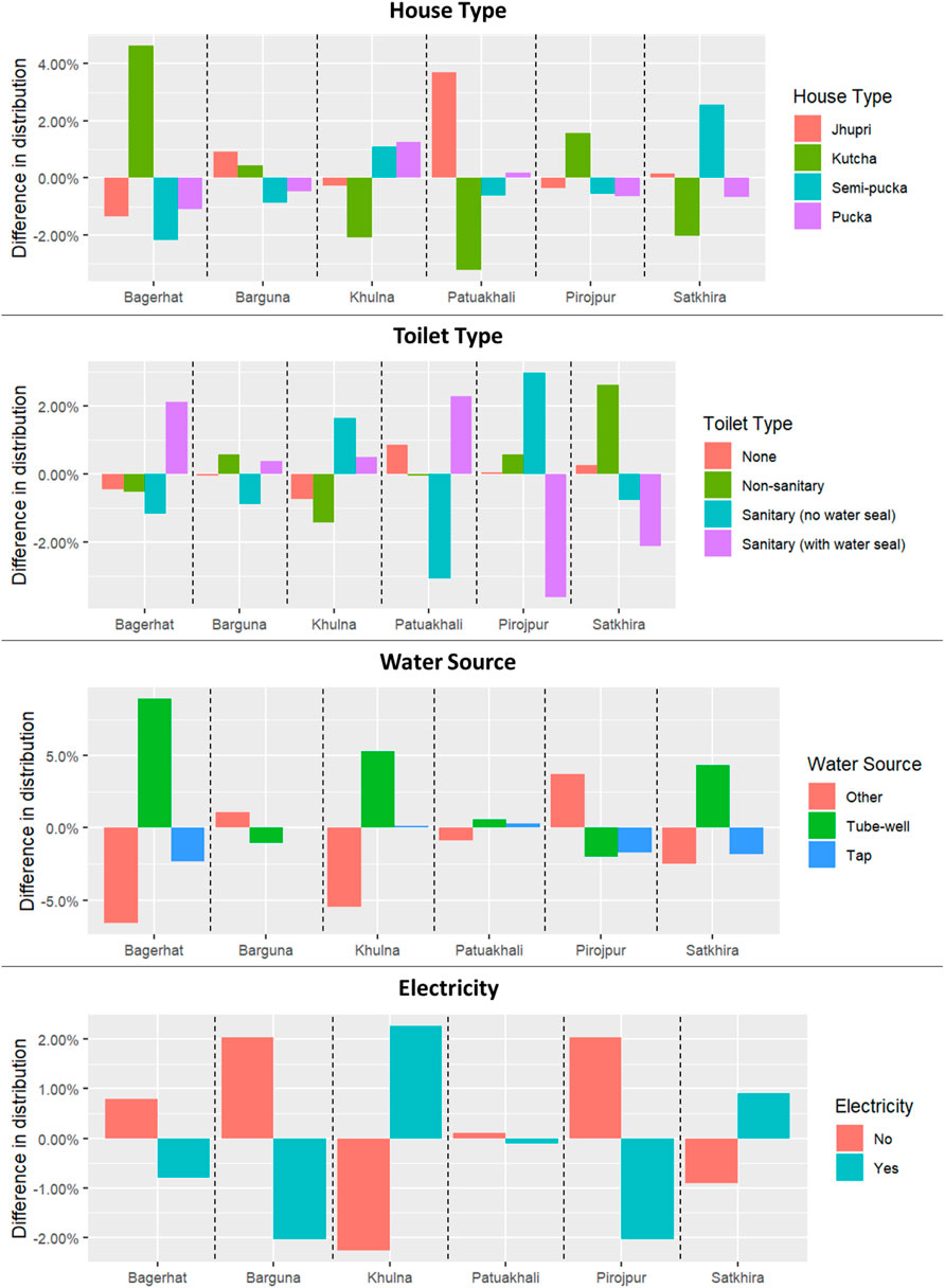
FIGURE 5. Difference from the expected distribution for variables of modelled potentially flooded households.
Discussion
In this study, we presented an integrated analytical approach for disaster risk analysis using a case study of six districts in the BCZ that were impacted by Cyclone Fani (2019). The methodology we proposed in this paper combines spatial microsimulation techniques for generating synthetic populations with dasymetric modelling techniques to determine the spatial distribution of populations through a dataset of spatially referenced synthetic households. This methodology allowed us to generate synthetic structural and socioeconomic microdata for around 9.5 million persons as point locations, which we overlayed with satellite-derived inundation maps of Cyclone Fani. We find that around 580 km2 of land was inundated, with six out of 49 upazilas having at least 10 percent of their surface area flooded. We further find that more than 100,000 households were exposed to flood inundation, predominantly living in kutcha housing, using tube-wells as drinking water source, living in rural areas and having no access to electricity. We find mixed results in terms of the exposure bias of households with certain household characteristics, which vary across to the district.
The approach we proposed in this paper represents the natural convergence between two prominent geospatial workarounds for better understanding household dynamics without having full access to detailed survey information. While this technique is exceedingly difficult to verify at lower resolutions, our study has the advantage of drawing upon a spatially referenced survey of households to verify both modelled location information and one associated household attribute (age) in a contained geographic area. However, despite efforts to validate the methodology, reliable validation data is hard to obtain. As such, while proving to be a suitable methodology to derive synthetic exposure and vulnerability estimates across large regions in a consistent way, it should be complemented with detailed household survey data before or after disasters to infer impacts to households and their socio-vulnerability, as is common practice in Bangladesh and elsewhere (Akter and Mallick, 2013).
Techniques for high-resolution dasymetric mapping are increasingly achievable at higher accuracy and at larger scales. On top of that, efforts such as IPUMS and other data repositories are encouraging the open release of microdata and cataloguing its availability for public usage. Still, public releases of census microdata only cover a small percentage of the total individuals and households for the aggregated unit (typically up to 10 percent), thus making population synthesis as presented in this study necessary to generate attributes for the entire population. Hence, we expect our methodology to be applicable across geographies that have reliable and high-resolution census information. From a human and computing capacity perspective, our methodology is set up so that it can be readily applied in a developing country context through the usage of pre-packaged tools within open-source software such as R and QGIS. Our model required approximately 20 total days to run for the combined study area. While computationally intensive at scale, it can be run for smaller populations (e.g., less than 50,000) on local computers. Most importantly, the methodology can be applied without a potentially costly software license, and once the dataset is generated, it can then be readily utilized by local practitioners for spatial analysis.
While SAE techniques can increase the resolution in which we understand the distribution of attributes, they are still restricted to the lowest level of disaggregation of the target data. In other words, they would not pick up on clusters and patterns of settlement location within the lowest area of disaggregation. This is particularly trye if one is interested in attributes which have strong spatial dependencies within a small administrative unit. For instance, in our study, the lowest level for disaggregation before the spatial randomization component is at the union council level in Bangladesh, which still encompasses relatively large areas compared to the inundation extent in some union councils. Hence, we expect some level of uncertainty in our estimates as we are restricted to this level for disaggregation. For spatial attributes with stronger potential spatial dependencies (e.g. wealth, water access, etc.) the spatial distribution can be further refined within the administrative unit by incorporating spatial modelling techniques which consider factors such as the spatial autocorrelation of selected attributes, dependencies related to additional known covariates (e.g. poorer households may live further from water access) or additional georeferenced surveys.
Our study takes the high resolution dasymetric population and spatial microsimulation approaches a step further by demonstrating a novel methodology for deriving synthetic households with unique geographic locations and socioeconomic attributes. However, our methodology for generating point coordinates comes at the expense of computational intensity. Going from disaggregated SAE estimates, in our case information at 436 union councils in our study area, towards individual (synthetic) household locations and attributes for 9.5 million people increases the data output and computational resources needed considerably, potential limiting the application of such methodologies to institutions that do have access to such computational resources. On top of that, uncertainties are not conveyed in the methodology because of this computational intensity. For instance, the uncertainty in the randomization component to assign households to point estimates within the respective union administrative boundary could be circumvented by creating multiple realization of the georeferenced synthetic population data, which was not possible given the computational resources needed in this study.
Despite the limitations, our approach can be applied to inform the response and recovery phases after disasters, where quick access to reliable aggregate figures is essential for coordinating relief efforts and large-scale resource mobilization. Modelled socioeconomic characteristics may provide utility in prioritizing specific and targeted actions when coordinating relief efforts (e.g. decisions as to where to provide temporary shelter, water, or sanitation services). In addition to providing utility in the response and recovery phases after natural disasters, our approach can be applied to inform ex-ante investments and associated policies focused on enhancing the resilience of vulnerable communities. Our modelled socioeconomic variables could contribute towards a multidimensional understanding of household poverty (Alkire and Foster, 2011) and socioeconomic resilience (Hallegatte et al., 2017). A better baseline understanding of where populations live, and their poverty incidence or socioeconomic vulnerability, could help inform decision-making concerning large-scale adaptation options (e.g. embankments, cyclone shelters) or softer adaptation solutions (e.g. cash transfer, social safety nets). More specifically, our methodology can help target such interventions such that they reduce the welfare impacts of poor populations (Verschuur et al., 2020).
In our work, we only observe a very small exposure bias of modelled potentially flooded households when compared to modelled non-flooded households. Although this conclusion is consistent with that of Winsemius et al. for rural flood events (Winsemius et al., 2018), it is in contrast to some of the literature in Bangladesh that did find an exposure bias for river flooding (Brouwer et al., 2007). This could be explained give that the random nature of cyclones makes the occurrence of an exposure bias less likely, as it less dependent on long-term structural conditions that might determine the location of a household (e.g. land prices).
Altogether, we showcase how combining high-resolution flood extent information, either from remote sensing or model output, combined with modelled socioeconomic characteristics of those populations exposed could provide novel insights into disproportionate hazard exposure. This could not only inform mapping the exposure of specific vulnerable populations, but also add value across the disaster risk management cycle to inform policy decision-making and investment planning.
Data availability statement
The datasets presented in this study can be found in online repositories. The names of the repository/repositories and accession number(s) can be found below: 10.6084/m9. figshare.11695356.
Author contributions
JG and AK were responsible for generating the synthetic populations. SR was responsible for spatially distributing synthetic populations to vector points, and RG, JM, and BB were responsible for mapping the flooded area from Cyclone Fani. SR conducted the spatial analysis and generated all figures for the Cyclone Fani case study. SR, JV, and JH were involved in formulating the results and implications. SR wrote the manuscript, with primary contributions from JV, RG, JG, and JH.
Acknowledgments
The authors acknowledge support from the REACH Program funded by United Kingdom Aid from the United Kingdom Department for International Development (DFID) for the benefit of developing countries (Aries Code 201880), the City Resilience Program (www.gfdrr.org/crp), the Global Facility for Disaster Reduction and Recovery, and the World Bank. However, the views expressed, and information contained in it, are not necessarily those of or endorsed by DFID, the City Resilience Program, the Global Facility for Disaster Reduction and Recovery, or the World Bank, which can accept no responsibility for such views or information or for any reliance placed on them. JV acknowledges funding from the Engineering and Physical Sciences Research Council (EPSRC) under grant number EP/R513295/1.
Conflict of interest
Authors RG, JM, and BB were employed by New Light Technologies Inc.
The remaining authors declare that the research was conducted in the absence of any commercial or financial relationships that could be construed as a potential conflict of interest.
Publisher’s note
All claims expressed in this article are solely those of the authors and do not necessarily represent those of their affiliated organizations, or those of the publisher, the editors and the reviewers. Any product that may be evaluated in this article, or claim that may be made by its manufacturer, is not guaranteed or endorsed by the publisher.
Supplementary material
The Supplementary Material for this article can be found online at: https://www.frontiersin.org/articles/10.3389/fenvs.2022.1033579/full#supplementary-material
References
Adams, H., Adger, W. N., Ahmad, S., Ahmed, A., Begum, D., Lázár, A. N., et al. (2016). Spatial and temporal dynamics of multidimensional well-being, livelihoods and ecosystem services in coastal Bangladesh. Sci. Data 3, 160094. doi:10.1038/sdata.2016.94
Akter, S., and Mallick, B. (2013). The poverty-vulnerability-resilience nexus: Evidence from Bangladesh. Ecol. Econ. 96, 114–124. doi:10.1016/j.ecolecon.2013.10.008
Alam, E., and Collins, A. E. (2010). Cyclone disaster vulnerability and response experiences in coastal Bangladesh. Disasters 34, 931–954. doi:10.1111/j.1467-7717.2010.01176.x
Alkire, S., and Foster, J. (2011). Understandings and misunderstandings of multidimensional poverty measurement. J. Econ. Inequal. 9, 289–314. doi:10.1007/s10888-011-9181-4
Arzberger, P., Schroeder, P., Beaulieu, A., Bowker, G., Casey, K., Laaksonen, L., et al. (2004). Promoting access to public research data for scientific, economic, and social development. Data Sci. J. 3, 135–152. doi:10.2481/dsj.3.135
Bangalore, M., Smith, A., and Veldkamp, T. (2016). Exposure to floods, climate change, and poverty in vietnam. Expo. Floods, Clim. Chang. Poverty Vietnam 3, 79–99. doi:10.1596/1813-9450-7765
Bangladesh Bureau of Statistics (2022). Bangladesh preliminary report of population census 2022. Dhaka, Bangladesh: Bangladesh Bureau of Statistics.
Bangladesh Bureau of Statistics (2012). Population and housing census 2011. Available at: http://203.112.218.66/WebTestApplication/userfiles/Image/BBS/Socio_Economic.pdf.
Barthelemy, J., and Toint, P. L. (2013). Synthetic population generation without a sample. Transp. Sci. 47, 266–279. doi:10.1287/trsc.1120.0408
Beckman, R. J., Baggerly, K. A., and McKay, M. D. (1996). Creating synthetic baseline populations. Transp. Res. Part A Policy Pract. 30, 415–429. doi:10.1016/0965-8564(96)00004-3
Brouwer, R., Akter, S., Brander, L., and Haque, E. (2007). Socioeconomic vulnerability and adaptation to environmental risk: A case study of climate change and flooding in Bangladesh. Risk Anal. 27, 313–326. doi:10.1111/j.1539-6924.2007.00884.x
Chini, M., Pelich, R., Pulvirenti, L., Pierdicca, N., Hostache, R., and Matgen, P. (2019). Sentinel-1 InSAR coherence to detect floodwater in urban areas: Houston and hurricane harvey as A test case. Remote Sens. (Basel). 11, 107. doi:10.3390/rs11020107
Clement, M. A., Kilsby, C. G., and Moore, P. (2018). Multi-temporal synthetic aperture radar flood mapping using change detection. J. Flood Risk Manag. 11, 152–168. doi:10.1111/jfr3.12303
Dasgupta, S., Huq, M., Khan, Z. H., Ahmed, M. M. Z., Mukherjee, N., Khan, M. F., et al. (2014). Cyclones in a changing climate: The case of Bangladesh. Clim. Dev. 6, 96–110. doi:10.1080/17565529.2013.868335
Dasgupta, S., Huq, M., Khan, Z. H., Ahmed, M. M. Z., Mukherjee, N., Khan, M. F., et al. (2010). Vulnerability of Bangladesh to cyclones in a changing climate potential damages and adaptation cost. Policy Res. Work. Pap. 5280, 54. doi:10.1111/j.1467-7717.1992.tb00400.x
Doxsey-Whitfield, E., MacManus, K., Adamo, S. B., Pistolesi, L., Squires, J., Borkovska, O., et al. (2015). Taking advantage of the improved availability of census data: A first look at the gridded population of the world, version 4. Pap. Appl. Geogr. 1, 226–234. doi:10.1080/23754931.2015.1014272
Dullaart, J. C. M., Muis, S., Bloemendaal, N., Chertova, M. V., Couasnon, A., and Aerts, J. C. J. H. (2021). Accounting for tropical cyclones more than doubles the global population exposed to low-probability coastal flooding. Commun. Earth Environ. 2, 135. doi:10.1038/s43247-021-00204-9
Elbers, C., Lanjouw, J. O., and Lanjouw, P. (2003). Micro-level estimation of poverty and inequality. Econometrica 71, 355–364. doi:10.1111/1468-0262.00399
Elbers, C., Lanjouw, P., and Leite, P. G. (2008). Brazil within Brazil: Testing the poverty map methodology in minas gerais. Washington: World Bank.
Esch, T., Heldens, W., Hirner, A., Keil, M., Marconcini, M., Roth, A., et al. (2017). Breaking new ground in mapping human settlements from space – the Global Urban Footprint. ISPRS J. Photogramm. Remote Sens. 134, 30–42. doi:10.1016/j.isprsjprs.2017.10.012
Formetta, G., and Feyen, L. (2019). Empirical evidence of declining global vulnerability to climate-related hazards. Glob. Environ. Change 57, 101920. doi:10.1016/j.gloenvcha.2019.05.004
Ghosh, M., and Rao, J. N. K. (1994). Small area estimation: An appraisal. Stat. Sci. 9, 647. doi:10.1214/ss/1177010647
Goodchild, M. F., Anselin, L., and Deichmann, U. (1993). A framework for the areal interpolation of socioeconomic data. Environ. Plan. A 25, 383–397. doi:10.1068/a250383
Grinberger, A. Y., Lichter, M., and Felsenstein, D. (2017). “Dynamic agent based simulation of an urban disaster using synthetic big data,” in Seeing cities through big data: Research, methods and applications in urban Informatics (Heidelberg: Springer), 349–382. doi:10.1007/978-3-319-40902-3_20
Hallegatte, S., and Rozenberg, J. (2017). Climate change through a poverty lens. Nat. Clim. Chang. 7, 250–256. doi:10.1038/nclimate3253
Hallegatte, S., Vogt-Schilb, A., Bangalore, M., and Rozenberg, J. (2017). Unbreakable: Building the resilience of the poor in the face of natural disasters. Washington, DC: World Bank. doi:10.1596/978-1-4648-1003-9
Hallegatte, S., Vogt-Schilb, A., Rozenberg, J., Bangalore, M., and Beaudet, C. (2020). From poverty to disaster and back: A review of the literature. Econ. Disaster. Clim. Chang. 4, 223–247. doi:10.1007/s41885-020-00060-5
Harland, K., Heppenstall, A., Smith, D., and Birkin, M. (2012). Creating realistic synthetic populations at varying spatial scales: A comparative critique of population synthesis techniques. J. Artif. Soc. Soc. Simul. 15, 1909. doi:10.18564/jasss.1909
Hossain, M. S., Johnson, F. A., Dearing, J. A., and Eigenbrod, F. (2016). Recent trends of human wellbeing in the Bangladesh delta. Environ. Dev. 17, 21–32. doi:10.1016/j.envdev.2015.09.008
Jongman, B., Ward, P. J., and Aerts, J. C. J. H. (2012). Global exposure to river and coastal flooding: Long term trends and changes. Glob. Environ. Change 22, 823–835. doi:10.1016/j.gloenvcha.2012.07.004
Khan, S. I., Hong, Y., Wang, J., Yilmaz, K. K., Gourley, J. J., Adler, R. F., et al. (2011). Satellite remote sensing and hydrologic modeling for flood inundation mapping in lake victoria basin: Implications for hydrologic prediction in ungauged basins. IEEE Trans. Geosci. Remote Sens. 49, 85–95. doi:10.1109/TGRS.2010.2057513
Lallemant, D., Soden, R., Rubinyi, S., Loos, S., Barns, K., and Bhattacharjee, G. (2017). Post-disaster damage assessments as catalysts for recovery: A look at assessments conducted in the wake of the 2015 gorkha, Nepal, Earthquake. Earthq. Spectra 33, 435–451. doi:10.1193/120316eqs222m
Lam, N. S.-N. (1983). Spatial interpolation methods: A review. Am. Cartogr. 10, 129–150. doi:10.1559/152304083783914958
Le De, L., Gaillard, J. C., Friesen, W., and Smith, F. M. (2015). Remittances in the face of disasters: A case study of rural Samoa. Environ. Dev. Sustain. 17, 653–672. doi:10.1007/s10668-014-9559-0
Lee, D., Ahmadul, H., Patz, J., and Block, P. (2021). Predicting social and health vulnerability to floods in Bangladesh. Nat. Hazards Earth Syst. Sci. 21, 1807–1823. doi:10.5194/nhess-21-1807-2021
Li, Y., Martinis, S., Plank, S., and Ludwig, R. (2018). An automatic change detection approach for rapid flood mapping in Sentinel-1 SAR data. Int. J. Appl. Earth Obs. Geoinf. 73, 123–135. doi:10.1016/j.jag.2018.05.023
Malmgren-Hansen, D., Sohnesen, T., Fisker, P., and Baez, J. (2020). Sentinel-1 change detection analysis for cyclone damage assessment in urban environments. Remote Sens. (Basel). 12, 2409. doi:10.3390/rs12152409
Markert, K. N., Chishtie, F., Anderson, E. R., Saah, D., and Griffin, R. E. (2018). On the merging of optical and SAR satellite imagery for surface water mapping applications. Results Phys. 9, 275–277. doi:10.1016/j.rinp.2018.02.054
Marzi, S., Mysiak, J., Essenfelder, A. H., Amadio, M., Giove, S., and Fekete, A. (2019). Constructing a comprehensive disaster resilience index: The case of Italy. PLoS One 14, 02215855–e221623. doi:10.1371/journal.pone.0221585
Melchiorri, M., Florczyk, A. J., Freire, S., Schiavina, M., Pesaresi, M., and Kemper, T. (2018). Unveiling 25 years of planetary urbanization with remote sensing: Perspectives from the global human settlement layer. Remote Sens. (Basel). 10, 768–819. doi:10.3390/rs10050768
Münnich, R., and Schürle, J. (2003). On the simulation of complex universes in the case of applying the German microcensus. Available at: https://d-nb.info/1162064749/34.
Pekel, J.-F., Cottam, A., Gorelick, N., and Belward, A. S. (2016). High-resolution mapping of global surface water and its long-term changes. Nature 540, 418–422. doi:10.1038/nature20584
Rentschler, J., Avner, P., Marconcini, M., Su, R., Strano, E., and Hallegatte, S. (2022a). Rapid urban growth in flood zones global evidence since 1985. Available at: http://www.worldbank.org/prwp.
Rentschler, J., Salhab, M., and Jafino, B. A. (2022b). Flood exposure and poverty in 188 countries. Nat. Commun. 13, 3527. doi:10.1038/s41467-022-30727-4
Schlaffer, S., Matgen, P., Hollaus, M., and Wagner, W. (2015). Flood detection from multi-temporal SAR data using harmonic analysis and change detection. Int. J. Appl. Earth Obs. Geoinf. 38, 15–24. doi:10.1016/j.jag.2014.12.001
Smith, A., Bates, P. D., Wing, O., Sampson, C., Quinn, N., and Neal, J. (2019). New estimates of flood exposure in developing countries using high-resolution population data. Nat. Commun. 10, 1814–1817. doi:10.1038/s41467-019-09282-y
Stevens, F. R., Gaughan, A. E., Linard, C., and Tatem, A. J. (2015). Disaggregating census data for population mapping using Random forests with remotely-sensed and ancillary data. PLoS One 10, 01070422–e107122. doi:10.1371/journal.pone.0107042
Tanoue, M., Hirabayashi, Y., and Ikeuchi, H. (2016). Global-scale river flood vulnerability in the last 50 years. Sci. Rep. 6, 36021–36029. doi:10.1038/srep36021
Tatem, A. J. (2017). WorldPop, open data for spatial demography. Sci. Data 4, 170004–170005. doi:10.1038/sdata.2017.4
Templ, M., Meindl, B., Kowarik, A., and Dupriez, O. (2017). Simulation of synthetic complex data: The R package simPop. J. Stat. Softw. 79, 10. doi:10.18637/jss.v079.i10
Thomson, D., Kools, L., and Jochem, W. (2018). Linking synthetic populations to household geolocations: A demonstration in Namibia. Data 3, 30. doi:10.3390/data3030030
Tiecke, T. G., Liu, X., Zhang, A., Gros, A., Li, N., Yetman, G., et al. (2017). Mapping the world population one building at a time. arXiv. doi:10.1596/33700
Twele, A., Cao, W., Plank, S., and Martinis, S. (2016). Sentinel-1-based flood mapping: A fully automated processing chain. Int. J. Remote Sens. 37, 2990–3004. doi:10.1080/01431161.2016.1192304
Uddin, M., Martin, M. A., and Meyer, F. J. (2019). Operational flood mapping using multi-temporal sentinel-1 SAR images: A case study from Bangladesh. Remote Sens. (Basel). 11, 1581. doi:10.3390/rs11131581
Verschuur, J., Koks, E. E., Haque, A., and Hall, J. W. (2020). Prioritising resilience policies to reduce welfare losses from natural disasters: A case study for coastal Bangladesh. Glob. Environ. Change 65, 102179. doi:10.1016/j.gloenvcha.2020.102179
Wheaton, W., Cajka, J., Chasteen, B., Wagener, D., Cooley, P., Ganapathi, L., et al. (2009). Synthesized population databases: A us geospatial database for agent-based models. Methods Rep. RTI. Press. 2009, 905. doi:10.3768/rtipress.2009.mr.0010.0905
Whitworth, A., Carter, E., Ballas, D., and Moon, G. (2017). Estimating uncertainty in spatial microsimulation approaches to small area estimation: A new approach to solving an old problem. Comput. Environ. Urban Syst. 63, 50–57. doi:10.1016/j.compenvurbsys.2016.06.004
Williamson, P., Mitchell, G., and McDonald, A. T. (2002). Domestic water demand forecasting: A static microsimulation approach. Water Environ. J. 16, 243–248. doi:10.1111/j.1747-6593.2002.tb00410.x
Winsemius, H. C., Jongman, B., Veldkamp, T. I. E., Hallegatte, S., Bangalore, M., and Ward, P. J. (2018). Disaster risk, climate change, and poverty: Assessing the global exposure of poor people to floods and droughts. Environ. Dev. Econ. 23, 328–348. doi:10.1017/S1355770X17000444
WorldPop (2017). Bangladesh 100m population, version 2. Available at: https://hub.worldpop.org/geodata/summary?id=94 (Accessed March 4, 2021).
Keywords: synthetic population, disaster risk management, Bangladesh, flooding, vulnerability
Citation: Rubinyi S, Verschuur J, Goldblatt R, Gussenbauer J, Kowarik A, Mannix J, Bottoms B and Hall J (2022) High-resolution synthetic population mapping for quantifying disparities in disaster impacts: An application in the Bangladesh Coastal Zone. Front. Environ. Sci. 10:1033579. doi: 10.3389/fenvs.2022.1033579
Received: 31 August 2022; Accepted: 08 November 2022;
Published: 24 November 2022.
Edited by:
Yizi Shang, China Institute of Water Resources and Hydropower Research, ChinaReviewed by:
Edris Alam, Rabdan Academy, United Arab EmiratesAnna Dmowska, Adam Mickiewicz University, Poland
Amy L. Griffin, RMIT University, Australia
Mingxing Hu, Southeast University, China
Rui A. P. Perdigão, Meteoceanics Institute for Complex System Science, Austria
Copyright © 2022 Rubinyi, Verschuur, Goldblatt, Gussenbauer, Kowarik, Mannix, Bottoms and Hall. This is an open-access article distributed under the terms of the Creative Commons Attribution License (CC BY). The use, distribution or reproduction in other forums is permitted, provided the original author(s) and the copyright owner(s) are credited and that the original publication in this journal is cited, in accordance with accepted academic practice. No use, distribution or reproduction is permitted which does not comply with these terms.
*Correspondence: Steven Rubinyi, c3RldmVuLnJ1YmlueWlAb3VjZS5veC5hYy51aw==