Correlation analysis and application investigation of multi-angle simultaneous polarization measurement data and concentration of suspended particulate matter in the atmosphere

Determining the composition, particle size distribution and concentration changes of suspended particulate matter in the atmosphere is important for evaluating the quality of air and its impact on public health. The scattering and absorption of light by suspended particulate matter can change the polarization state of light, which can be used to extract characteristic information of measured particles. Firstly, we use our previously developed multi-angle simultaneous polarization measurement device to monitor the particulate matter around Dianshan Lake, Shanghai, and obtain high-throughput, high-dimensional Stokes data for nearly 1 month. The correlation between the Stokes data measured and the reference concentrations of five suspended particulate matter (Si, K, Fe, Ca, and Zn) was analyzed using the Periodical canonical correlation analysis (PCCA) method. The study shows a strong correlation between the three Stokes vectors and the concentrations of two types of suspended particulate matter in the atmosphere. Moreover, a prediction model for the concentration change of suspended particles was proposed by combining the locally weighted linear regression (LWLR) and the auto regressive moving average (ARMA) model. The prediction results on the concentration change of K and Fe in the atmosphere verified the validity of our method. The research in this work offers the possibility of continuous analysis and prediction of atmospheric suspended particulate matter in real environments.

1 Introduction

Aerosols are solid or liquid suspended particulate matter dispersed uniformly in the air. It is important to determine the composition, source and concentration variation of aerosols to evaluate the quality of the atmosphere. The main types of aerosols are carbonaceous aerosols, secondary inorganic water-soluble aerosols, sea salt aerosols, biomass aerosols and mineral dust aerosols. The aerosols have an important impact on climate, visibility, radiative forcing, photochemical smog production, and ecosystem damage (Haywood and Boucher, 2000; Mauderly and Chow, 2008). Secondary inorganic water-soluble aerosols mainly include sulfate and nitrate, which are important contributors to haze production (Fowler et al., 2013; Shang et al., 2020). The main components of sea salt aerosols include NaCl and NaBr, in which halide ions are photolyzed to produce halogen atoms, which in turn have the potential to affect ozone levels in the troposphere (Thomas et al., 2007). Bioaerosols may consist of bacteria, fungi, viruses, pollen, plant fibers, etc. Bioaerosol exposure may produce infectious diseases, acute poisoning, allergies, or cancers with public health implications (Douwes et al., 2003). Mineral dust aerosols are chemically stable and consist mainly of oxides of elements such as silicon (Si), potassium(K), iron (Fe), aluminum (Al), magnesium (Mg), sodium (Na), calcium (Ca) and zinc (Zn), and can be generated by natural means such as soil dust, sandstorms, volcanic eruptions or by anthropogenic means such as bituminous coal dust or construction cement dust (Wang et al., 2008; Miffre et al., 2012). Airborne particulate matter (PM), which is often complex in composition and varies over time and space, is a major cause of environmental pollution and has many health risks. For example, PM2.5 (particulate matter with an aerodynamic diameter of less than 2.5 microns) can cause respiratory illnesses such as shortness of breath, chest discomfort, coughing and wheezing (Guaita et al., 2011), as well as cardiovascular diseases such as congestive heart failure (Wellenius et al., 2005), atherosclerosis (Suwa et al., 2002), and leads to decreased vagal tone with reduced heart rate variability (Gold et al., 2000). Therefore, testing the composition, concentration and particle size distribution of suspended particulate matter in the atmosphere can help to assess the impact of suspended particulate matter on human health and thus provide advice to environmental regulators on policy development.

The two main types of methods commonly used to carry out suspended particulate matter testing are sampling and non-sampling methods. Common sampling methods include filter membrane methods, piezoelectric crystal methods, β -ray absorption methods and micro-oscillation balance methods (Olin and Sem, 1971; Patashnick and Rupprecht, 2012; Gao et al., 2017), whose detection accuracy of sampling methods is generally high, but the process is cumbersome and the monitoring is poor in real time. For non-sampling detection, optical techniques provide a good way to achieve non-invasive and high-throughput analysis, such as extinction spectroscopy, photoacoustic spectroscopy, flow cytometry, and light scattering (Berthet et al., 2002; Green et al., 2003; Xue et al., 2016; Woźniak et al., 2018). Recently, polarization measurement shows great potential in particle analysis due to its advantages of no tagging, high information dimensionality, and easy retrofitting from the original light scattering detection device. In our previous research work, we develop a measurement system based on multi-angle optical scattering and multidimensional polarization analyzing technique (Li et al., 2019). Based on this, Guo et al. (2022) simultaneously inverted the complex refractive index and particle size distribution of suspended particulate matter by multi-angle polarization scattering measurements. And Xu et al. (2021) used machine learning methods to process high-throughput multi-angle single particle polarization scattering signals to achieve real-time online identification of individual suspended particulate matter.

In this paper, the detection of suspended particulate matter in the outdoor atmosphere around Dianshan Lake in Shanghai was carried out using our developed device. To obtain 8-dimensional high-throughput Stokes data. A new method to analyze the correlation between high-throughput and high-dimensional variables is proposed using five types of airborne suspended particulate matter concentration data given by local particle monitoring superstation as reference data. We obtained a high correlation between certain Stokes data and particulate matter reference concentration data. Finally, Based on the Stokes data measured by our equipment, we made preliminary predictions of the changes in the concentration of two suspended particulate matter (K, Fe) in the outdoor atmosphere, demonstrating the feasibility of our suspended particulate matter measurements for real environment monitoring and prediction.

2 Methods

2.1 Periodical canonical correlation analysis method

The data set used in this experiment is the polarized light data of outdoor airborne suspended particulate matter measured by our device and the data of airborne suspended particulate matter (Si, K, Fe, Ca, and Zn) provided by the Shanghai Environmental Monitoring Center. The concentrations of Si, K, Fe, Ca, and Zn were measured by the Shanghai Environmental Monitoring Center using an airborne elemental analysis monitoring device (Xact625, Cooper Environmental Services LLC, United States), which main measurement principle is based on the X-Ray Fluorescence (XRF) method. The data given by the Shanghai Environmental Monitoring Center are the concentration data of suspended particulate matter in the outdoor atmosphere. The polarized light data contain 8 polarization parameters for the H-polarized state incidence and 8 polarization parameters for the P-polarized state incidence, respectively.

The Schematic diagram of the single particle measurement method for suspended particulate matter in the atmosphere is shown in Figure 1. First, the light from the laser (532 nm, 100 mW, MSL-III-532, CNI) passes through the PSG, C and detection area, and is then collected by the light trap. When a single particle passes through the detection zone, the light intensity channel will be triggered, and then P1-P4 start to collect the polarized light. Combining the incident polarized light and the collected exiting polarized light, we can obtain information about the suspended particulate matter in the atmosphere. The properties of polarized light can usually be expressed by a Stokes vector, which is calculated by adding and subtracting the light intensities of different components, which is described by Eq. 1. The index represents the polarization state of the polarization state analyzer, where 0°, 45°, 90° and 135° represent the linear polarization state; R and L represent the right-handed and the left-handed circular polarization state.

$\mathit{S}=\left[\begin{array}{c}{\mathit{s}}_{\mathbf{0}}\\ {\mathit{s}}_{\mathbf{1}}\\ {\mathit{s}}_{\mathbf{2}}\\ {\mathit{s}}_{\mathbf{3}}\end{array}\right]=\left[\begin{array}{c}{\mathit{I}}_{\mathbf{0}}+{\mathit{I}}_{\mathbf{90}}\\ {\mathit{I}}_{\mathbf{0}}-{\mathit{I}}_{\mathbf{90}}\\ {\mathit{I}}_{\mathbf{45}}-{\mathit{I}}_{\mathbf{135}}\\ {\mathit{I}}_{\mathit{R}}-{\mathit{I}}_{\mathit{L}}\end{array}\right](1)$

FIGURE 1

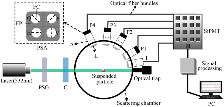
FIGURE 1. Schematic diagram of the single particle measurement method for suspended particulate matter in the atmosphere. PSG, polarization state generator; C, cylindrical lens; I, light intensity channel (10°); L, biconvex lens; A, aperture; P1-P4, polarization state analysis channel for 30°, 60°, 85°, 115°, respectively; PSA, polarization state analyzer; FP, polarizer film; FC, fiber core; H, horizontal polarizer film; V, vertical polarizer film; P, 45° polarizer film; Q, 135° polarizer film; SiPMT, silicon photomultiplier tube; OPS, optical particle sizer.

In this work, for comparison with the reference data provided by the monitoring station, we averaged the measured multiple-scattering angle Stokes vectors s₁ and s₂ by hour.

Before using the polarized light data to predict airborne particulate matter concentrations, it is necessary to analyze the correlation between the polarized light data and the reference data given by the Shanghai Environmental Monitoring Center which will help to improve the accuracy of the prediction. The simplest way to analyze the correlation between data is the Pearson correlation method, but the Pearson correlation can only analyze the correlation between two columns of data, but not the correlation between two multidimensional data sets as a whole. Hotelling first proposed the canonical correlation analysis (CCA) method (Hotelling, 1936), which is similar to the PCA downscaling technique and can explore the correlation between two sets of variables. The CCA method is a multivariate statistical technique that allows the study of relationships between multiple dependent variables and multiple independent variables. The CCA method can find linear combinations of two sets of variables with maximum Pearson correlation (Ahmadianfar et al., 2020). CCA constructs linear combinations from two sets to maximize the correlation between the two sets. The linear combinations in the two sets are ranked according to the magnitude of the correlation, and the linear combination pair with the greatest correlation is obtained, called the typical variable pair (U1, V1; U2, V2; U3, V3 ...).

The two most important parameters in the canonical correlation analysis are the typical load factor and the explanatory factor. The typical load factor (Tlf) is used to specify the correlation between the typical variables and the input indicators, and Tlf is calculated as Eq. 2 The larger the absolute value of the Tlf, the stronger the correlation between this item and the typical variables. The explanatory factor (Ef) is used to measure the ability of the typical variable to explain the information contained in all the input indicators, the larger the Ef the stronger the typical variable’s ability to explain the information contained in the input indicators. The explanatory factor is also known as the variance explained ratio and is calculated as shown in Eq. 3.

${\mathit{T}\mathit{l}\mathit{f}}_{\mathit{X}\mathit{U}}=\frac{\mathbf{1}}{\mathit{n}}{\sum }_{\mathit{i}=\mathbf{1}}^{\mathit{n}}\frac{\left({\mathit{X}}_{\mathit{i}}-\mathit{E}\left(\mathit{X}\right)\right)}{{\mathit{\sigma }}_{\mathit{X}}}\bullet \frac{\left({\mathit{U}}_{\mathit{i}}-\mathit{E}\left(\mathit{U}\right)\right)}{{\mathit{\sigma }}_{\mathit{U}}}(2)$

${\mathit{E}\mathit{f}}_{\mathit{k}}=\frac{\mathbf{1}}{\mathit{n}}{\sum }_{\mathit{i}=\mathbf{1}}^{\mathit{n}}{\mathit{T}\mathit{l}\mathit{f}}_{{\mathit{X}}_{\mathit{i}}{\mathit{U}}_{\mathit{k}}}(3)$

σ_X and σ_Y are the variances of the X and Y vectors respectively, and X and U are column vectors. Combining Eqs 2, 3, the typical load interpretation factor (Tlif) is defined in this paper, as shown in Eq. 4.

${\mathit{T}\mathit{l}\mathit{i}\mathit{f}}_{\mathit{X}{\mathit{U}}_{\mathit{k}}}=\left({\mathit{E}\mathit{f}}_{\mathit{k}}\right)\bullet {\left({\mathit{T}\mathit{l}\mathit{f}}_{\mathit{X}{\mathit{U}}_{\mathit{k}}}\right)}^{\mathbf{2}}(4)$

The typical load interpretation factor is obtained by multiplying the explanatory factor and the square of the typical load factor, so that it not only reflects the high correlation between the typical variable and the original data, but also the degree of trustworthiness of this correlation. If the typical load factor is large, but the explanatory factor is small, it means that the typical variable is highly correlated with the original data, but the typical variable contains less information about the original data, indicating that this correlation is not reliable. Similarly, if the typical load factor is small, but the explanatory factor is large, which means the correlation between the typical variable and the original data is low, but the typical variable contains more information about the original data, indicating that the correlation is not very reliable. In contrast, the typical load interpretation factor combines the characteristics of the typical load factor and the explanatory factor, and can better characterize the correlation between the typical variables and the original data.

In this paper, periodical canonical correlation analysis (PCCA) is proposed based on the CCA method. PCCA is used to obtain typical load interpretation factors by calculating typical load factors and explanatory factors for multiple periods obtained from CCA analysis. By analyzing the statistical patterns of the typical load interpretation factors, the correlations between the two groups of variables analyzed are then obtained. In contrast to CCA, PCCA uses the statistics of multiple local correlations to analyze the correlation between two sets of variables, allowing more detailed correlation information to be uncovered within the data set. A schematic diagram of the whole PCCA calculation process is shown in Figure 2.

FIGURE 2

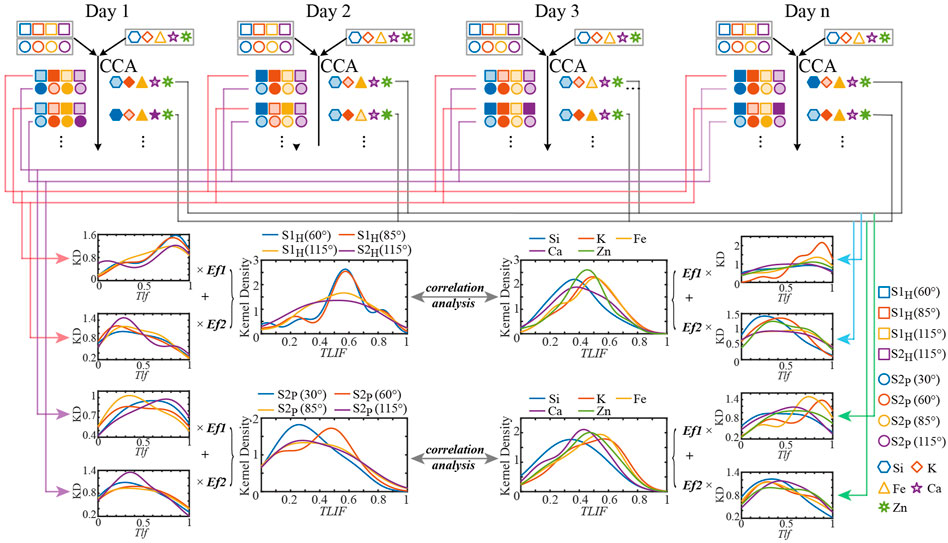
FIGURE 2. Schematic diagram of PCCA. CCA, canonical correlation analysis; KD, kernel density; Tlf, typical load factor; Ef, explanatory factor; TLIF, typical load interpretation factor.

As shown in Figure 2, PCCA works by first calculating typical load interpretation factors, Tlif1_XU, Tlif2_XU, … , Tlifp_XU, Tlif1_YV, Tlif2_YV, … , Tlifp_YV for each Stokes vector and suspended particulate matter, using the four Stokes vectors and the concentration data of suspended particulate matter for the first day of H incidence or P incidence, where p is the number of typical variable pairs, X is the name of the Stokes vector, Y is the name of the suspended particulate matter, U represents the typical variable corresponding to the Stokes vector, and V represents the typical variable corresponding to the concentration of the suspended particulate matter, and 1, 2, ... represents the ordinal number of the typical variable pair. This is done in turn until a typical load interpretation factor of each Stokes vector and suspended particulate matter is calculated for day n. Considering the effect of the explanatory factors, define:

${\mathit{T}\mathit{l}\mathit{i}\mathit{f}}_{\mathit{X}}={\sum }_{\mathit{k}=\mathbf{1}}^{\mathit{m}}{\mathit{T}\mathit{l}\mathit{i}\mathit{f}\mathit{k}}_{\mathit{X}\mathit{U}}(5)$

${\mathit{T}\mathit{l}\mathit{i}\mathit{f}}_{\mathit{Y}}={\sum }_{\mathit{k}=\mathbf{1}}^{\mathit{m}}{\mathit{T}\mathit{l}\mathit{i}\mathit{f}\mathit{k}}_{\mathit{Y}\mathit{V}}(6)$

In Eqs 5, 6, m indicates that the first m typical variable pairs with the largest correlation coefficients are selected to be counted as the typical load interpretation factor for each Stokes vector or suspended particulate matter. m can be selected based on the explanatory factor to ensure that the first m typical variable pairs explain enough information about the Stokes vector or suspended particulate matter concentration.

Thus, it is possible to calculate, Tlif_S1H(60°), …, Tlif_S2H(115°), Tlif_Si, … , Tlif_Zn and Tlif_S2P(30°), …, Tlif_S2P(115°), Tlif_Si, … , Tlif_Zn, respectively. The kernel density of each typical load interpretation factor is then plotted separately to find the ranking of the typical load interpretation factors corresponding to the peaks of the kernel density curves. The top groups with the largest typical load interpretation factors corresponding to the peaks of the kernel density curves indicate that these groups of Stokes vectors have the highest correlation with the suspended particulate matter.

2.2 Locally weighted linear regression methods

Linear regression is prone to underfitting because it seeks an unbiased estimate with a minimum mean square error. If the model is under-fitted, it will not achieve the best prediction results. Therefore some methods allow some bias to be introduced into the estimation, thus reducing the mean square error of the prediction and improving the prediction accuracy (Wang et al., 2016). Locally weighted linear regression is an improvement on standard linear regression, which solves the problem of under-fitting of standard linear regression and improves the prediction accuracy. The method accomplishes local fitting by assigning a certain weight to each point around the point to be measured and then performing an ordinary regression based on the minimum mean squared error on this subset. Locally weighted linear regression uses a moving average calculation similar to that of a time series, and a local fit can estimate a broader class of regression curves than a polynomial fit (Cleveland and Devlin, 1988). The basic principles of locally weighted linear regression are as follows:

Given the input vector x, the hypothesis function of the regression is denoted by $h_{\theta }\left(x\right)$, defined as

$\mathit{y}={\mathit{h}}_{\mathit{\theta }}\left(\mathit{X}\right)={\mathit{\theta }}^{\mathit{T}}\mathit{X}(7)$

where y is the vector to be regressed fitted, y = {y₁,y₂,...,y_n}, and X = {x₁,x₂,...,x_m} is the matrix of input independent variables, x₁ = x₁₁,x₁₂,...,x_1n. Thus, a vector of regression coefficients can be found $\theta$ that minimizes the mean squared error between the predicted and true values. Based on existing knowledge, it is known that the vector of regression coefficients obtained by linear regression $\theta$ is $\widehat{\theta }$ = (X^TX)⁻¹X^Ty. The small marker above $\theta$ indicates that this is the currently estimable $\theta$ of the optimal solution. Because the estimate $\theta$ from the available data may not be the true $\theta$ value, a “cap” symbol is used to indicate that it is only the best estimate of $\theta$. While the vector $\theta$ of regression coefficients resolved using the locally weighted linear regression algorithm is:

$\widehat{\mathit{\theta }}={\left({\mathit{X}}^{\mathit{T}}\mathit{W}\mathit{X}\right)}^{-\mathbf{1}}{\mathit{X}}^{\mathit{T}}\mathit{W}\mathit{y}.(8)$

LWLR uses a “kernel” similar to that used in support vector machines to give higher weights to nearby points. The type of kernel function can be freely chosen, and for regression prediction models, the choice of a suitable kernel function can effectively improve the prediction accuracy, with typical kernel functions being Gaussian, Exponential, and Laplace (Huang et al., 2020). The kernel function used in this paper is the Gaussian kernel function, and the corresponding weights of the Gaussian kernel function are as follows:

$\mathit{w}\left(\mathit{i},\mathit{i}\right)=\mathit{exp}\left(\frac{\left|{\mathit{x}}^{\left(\mathit{i}\right)}-\mathit{x}\right|}{-\mathbf{2}{\mathit{k}}^{\mathbf{2}}}\right)(9)$

This constructs a weight matrix W with only diagonal elements, W can assign a weight to each sample point and the closer the point x is to the other points, the greater the value w (i,i). Eq. 9 contains a parameter k to be formulated by the user that determines how much weight to assign to nearby points, and this is the only parameter that needs to be considered when using LWLR (Harrington, 2012). The relationship between the parameter k and the weights can be seen in Figure 3.

FIGURE 3

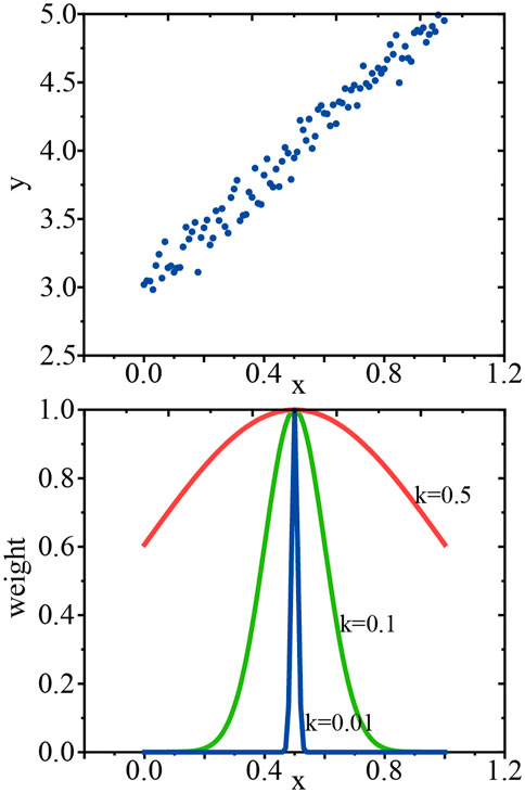
FIGURE 3. Relationship between parameter k and weights. The above panel represents the scatter plot of y and x; the bottom panel illustrates the changes in the weights of the points near the measurement point with the parameter k.

As shown in Figure 3, assuming that the point we are predicting is x = 0.5, the top plot shows the original data set. The bottom plot shows that when k = 0.5, most of the data is used to train the regression model; while when k = 0.01, only a small number of local points are used to train the regression model. When the chosen k parameter is large, the fitting result is similar to that of the least squares method, which is prone to overfitting; when the chosen k parameter is small, it is prone to overfitting and introduces a large number of noisy signals. Therefore, choosing the appropriate parameter k is beneficial to explore the potential laws of the data itself and improve the accuracy of the prediction results.

2.3 Auto regressive moving average models

The auto regressive moving average (ARMA) model is one of the typical models used to predict the trend of a time series (Hu et al., 2020). The general form of the ARMA model is ARMA (p,q), which is expressed as follows.

${\mathbf{x}}_{\mathbf{t}}=\left({\mathbf{\phi }}_{\mathbf{1}}{\mathbf{x}}_{\mathbf{t}-\mathbf{1}}+{\mathbf{\phi }}_{\mathbf{2}}{\mathbf{x}}_{\mathbf{t}-\mathbf{2}}+\cdots +{\mathbf{\phi }}_{\mathbf{p}}{\mathbf{x}}_{\mathbf{t}-\mathbf{p}}\right)+\left({\mathbf{\epsilon }}_{\mathbf{t}}-{\mathbf{\theta }}_{\mathbf{1}}{\mathbf{\epsilon }}_{\mathbf{t}-\mathbf{1}}-{\mathbf{\theta }}_{\mathbf{2}}{\mathbf{\epsilon }}_{\mathbf{t}-\mathbf{2}}-\cdots -{\mathbf{\theta }}_{\mathbf{q}}{\mathbf{\epsilon }}_{\mathbf{t}-\mathbf{q}}\right)(10)$

In Eq. 10, the model is an AR(p) model when q = 0 and an MA(q) model when p = 0. ${\phi }_1$, ${\phi }_2$,…, ${\phi }_p$ are the auto regressive coefficients, ${\theta }_1$, ${\theta }_2$,…, ${\theta }_q$ are the moving average coefficients. ε_t, ε_t-1, … , ε_t-q are random disturbance sequences. x_t-1, x_t-2, … , x_t-p are the past sequence values. The algorithm flow to predict chemical concentrations using the ARMA algorithm is shown in Figure 4.

FIGURE 4

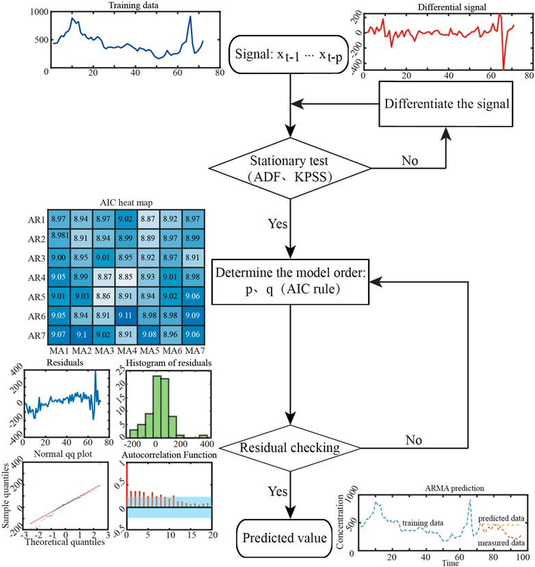
FIGURE 4. Flow chart of ARMA prediction algorithm.

As shown in Figure 4, when using the ARMA algorithm for series prediction, the smoothness of the signal is first tested using the ADF or KPSS method. It is worth noting that if the original signal does not pass the smoothness test, the original signal needs to be processed using the difference method until the result is smooth. Once the smoothness test is completed, the order of the ARMA model needs to be determined. ARMA models are generally of unknown order p and q and are usually derived recursively. Common criteria for determining whether the order is appropriate are Akaike’s information criterion (AIC), Akaike’s final prediction error (FPE), and the Bayes information criterion (BIC) (De Gooijer and Hyndman, 2006). In this paper, the AIC criterion is used, and the expression for AIC is:

$\mathit{A}\mathit{I}\mathit{C}\left(\mathit{k}\right)=\mathit{N}\mathit{l}\mathit{n}\left({\mathit{\rho }}_{\mathit{k}}\right)+\mathbf{2}\mathit{k}(11)$

In Eq. 11, N is the length of the data. As the order k increases from 1, AIC(k) will obtain a minimum value at some k, at which point k will be set to the most appropriate order. ${\rho }_k$ is the mean square value of the error series at order k, calculated as shown in Eq. 12.

${\mathit{\rho }}_{\mathit{k}}=\mathit{E}\left\{{\left[(\mathit{x}\left(\mathit{n}\right)-\widehat{\mathit{x}}\left(\mathit{n}\right))\right]}^{\mathbf{2}}\right\}(12)$

x(n) is the actual observed value, and $\widehat{x}\left(n\right)$ is the result calculated by a specific ARMA model. After determining the order p and q of the AMRA model, it is also necessary to check whether the model is a good fit. A common check method is the residual test, which is mainly to check the normality and irrelevance of the residuals. If the model fits adequately, the residual series follows a zero-mean-normal distribution and is completely random and uncorrelated. In this paper, the ARMA model is used to predict changes in the concentration of suspended particulate matter in the outdoor atmosphere, and its predictions are used as a reference value to adjust the parameter k of the LWLR prediction method.

3 Result

3.1 Correlation between Stokes vectors and suspended particulate matter concentrations

Using the PCCA method, it is necessary to select the first few pairs of typical variables to calculate the typical load interpretation factors. As shown in Figure 5, the box plots of the explanatory factors of the Stokes vector and suspended particulate matter concentration at H incidence and P incidence are plotted. From Figure 5, we can see the first two typical pairs of variables explain most of the raw data information, so m = 2 is set in Eqs 5, 6. Therefore, the first two typical load interpretation factors for all data were selected and summed as the typical load interpretation factors for the Stokes vector and suspended particulate matters’ concentration for each incident case, and then the kernel density curves for the typical load interpretation factors were plotted. Figure 6 shows how the PCCA method was applied to analyze the correlation between the Stokes vectors and suspended particulate matter concentrations.

FIGURE 5

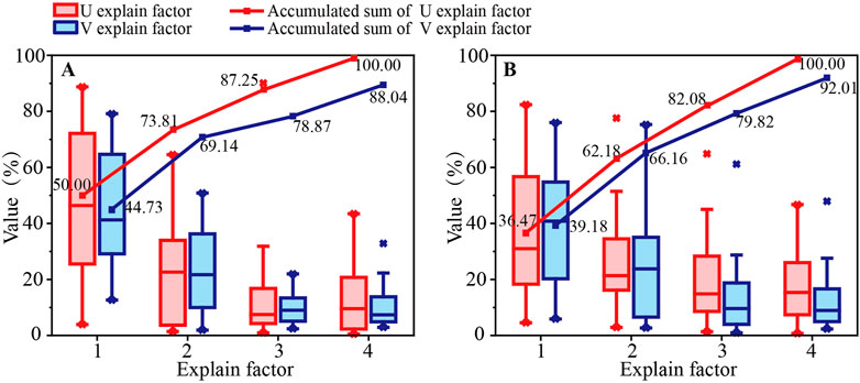
FIGURE 5. Box plots of the explanatory factors for typical variables derived for H incidence and P incidence. (A) panel shows the box plot of the explanatory factor for the case of H incidence, and (B) panel shows the case of P incidence.

FIGURE 6

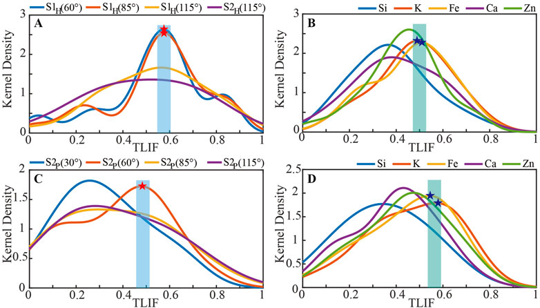
FIGURE 6. Typical load interpretation factor kernel density curves for Stokes vectors derived for H incidence and P incidence and suspended matters’ concentration. (A,B) show the results of PCCA under H incidence, (C,D) show the results of PCCA under P incidence.

Figures 6A,B indicate that the Stokes S1_H (60°) and S1_H (85°) peaks correspond to larger value range of TLIF in the case of H incidence, while the suspended particulate matter K and Fe peaks correspond to larger value range of TLIF. From the PCCA analysis of Section 2.1, the correlation between S1_H (60°), S1_H (85°) and K, Fe is high. Figures 6C,D show that in the case of P incidence, the Stokes S2_P (60°) peak corresponds to a larger value range of TLIF, and the suspended particulate matter K and Fe peaks correspond to larger value range of TLIF. Similarly, we can obtain that the correlation between S2_P (60°) and K, Fe is higher. Combining the above analysis, it can be concluded that the Stokes vectors S1_H (60°), S1_H (85°) and S2_P (60°) are highly correlated with the concentration of suspended particulate matter K and Fe in the outdoor atmosphere.

3.2 Predicting results based on ARMA & LWLR methods

3.2.1 Data preparation

Firstly, the data need to be preprocessed for outliers by removing the outlier points based on quadratic polar difference detection and then filling the data using triple spline interpolation. The before and after preprocessed curves are shown in Figure 7. The upper limit of quadrature polarization for outliers is Q3+1.5Iqr, and the lower limit is Q1-1.5Iqr. Any data that lies outside the lower and upper limits of the determination will be considered outliers. Q1, Q3 and Iqr are upper quartile, lower quartile, and the distance between the upper and lower quartiles respectively. As shown in Figure 7F, quadratic polarization-based outlier detection and removal, followed by triple spline interpolation, can effectively weaken the spikes in the original data compared, and still retain the trend and detailed information of the original data variation.

FIGURE 7

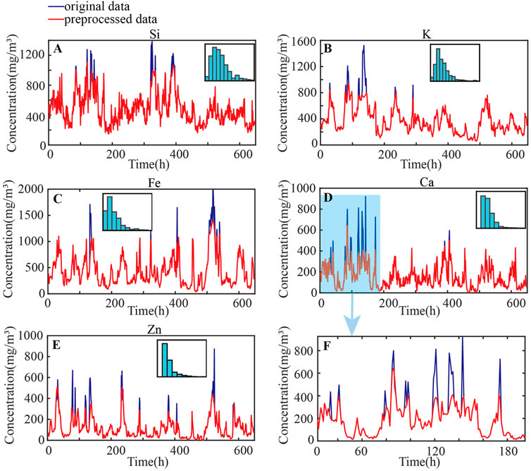
FIGURE 7. Preprocessing of outliers from raw chemical data. (A–E) show the changes in the concentration values with time (648 h for each) of Si, K, Fe, Ca, and Zn before and after preprocessing, respectively; the subplots of (A–E) show the concentration distribution of Si, K, Fe, Ca, and Zn, respectively; (F) is the local zoom of (D).

3.2.2 Predictions for the concentration of K and Fe

From Section 3.1 we know that the Stokes vectors S1_H (60°), S1_H (85°) and S2_P (60°) are highly correlated with changes in the concentrations of suspended particulate matter K and Fe. Next, we attempt to use the measured S1_H (60°), S1_H (85°) and S2_P (60°) to predict the changes in the concentration of K and Fe. Firstly, using the ARMA model combined with the past data of suspended particle concentrations, the predicted concentration values of suspended particles are shown in Figures 8A,D. Then the LWLR was used to predict the suspended particulate matter concentration values. By combining the past particulate concentration data with the Stokes data, the mean absolute percentage error (MAPE) between the ARMA predictions and the LWLR predictions can be calculated. It should be noted that MAPE was calculated using k = 0.001 as the initial value and incrementing parameter k with step = 0.001, the corresponding results are shown in Figures 8B,E. The minimum point of the MAPE curve, marked with red pentagrams in Figures 8B,E, and the corresponding parameter k are used as the final weight parameter for LWLR prediction to predict the concentration value of the suspended particulate matter, and the final prediction results can be obtained (Figures 8C,F). The formula for calculating MAPE is shown in Eq. 13

$\mathit{M}\mathit{A}\mathit{P}\mathit{E}={\sum }_{\mathit{t}=\mathbf{1}}^{\mathit{n}}\left|\frac{{\mathbf{m}\mathbf{e}\mathbf{a}\mathbf{s}\mathbf{u}\mathbf{r}\mathbf{e}\mathbf{d}}_{\mathit{t}}-{\mathbf{p}\mathbf{r}\mathbf{e}\mathbf{d}\mathbf{i}\mathbf{c}\mathbf{t}\mathbf{e}\mathbf{d}}_{\mathit{t}}}{{\mathbf{m}\mathbf{e}\mathbf{a}\mathbf{s}\mathbf{u}\mathbf{r}\mathbf{e}\mathbf{d}}_{\mathit{t}}}\right|\times \frac{\mathbf{100}}{\mathit{n}}(13)$

FIGURE 8

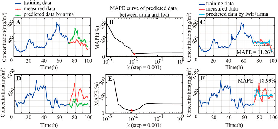
FIGURE 8. Comparison of measured concentrations and predicted concentrations based on the ARMA & LWLR method (K and Fe). (A,D) show the results before and after prediction by arma of K and Fe, respectively; (B,E) show the process of finding the most suitable parameter k of K and Fe, respectively; (C,F) show the results before and after prediction by lwlr + arma of K and Fe, respectively.

From Figures 8B,E, the variation of MAPE with parameter k is an overall upwardly concave curve with a unique minimum point. Here the length of training time chosen for the predictions was 3 days (72 h) and the time length of prediction was 1 day (24 h). According to Figures 8A,D, the error between the predicted trends in K and Fe concentration based on ARMA method and the measured value is larger (MAPE of K is 36.37%, while Fe is 48.96%). However, Figures 8C,F indicate that the ARMA & LWLR method can realize smaller errors between the predicted values and the measured values (MAPE of K is 11.26%, while Fe is 18.99%). Meanwhile, the overall trend of the predicted values is generally consistent with that of the measured data. Therefore, the prediction results are relatively reliable.

4 Discussion

4.1 Discussion on correlation analysis

In this section, we attempt to analyse the reasons for the relatively low correlation between Si, Ca, Zn and Stokes vector data in terms of data structure. In this paper, the first-order difference of the raw data is used to measure the degree and frequency of data mutation, and the kurtosis of the first-order difference distribution is used to quantify the analysis. Figure 9 shows the first-order difference and its kernel density function distribution for the five concentration data for suspended particulate matter (Si, K, Fe, Ca, and Zn).

FIGURE 9

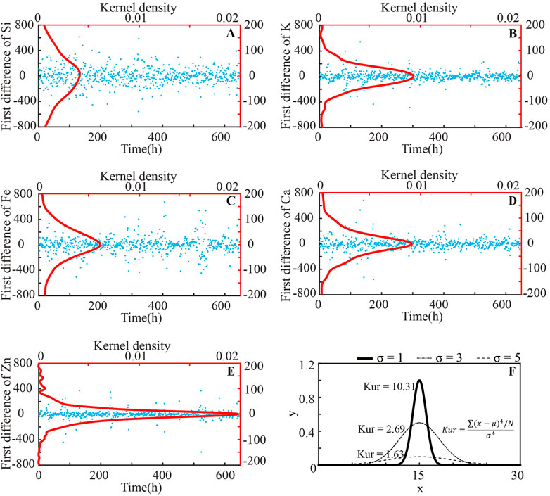
FIGURE 9. First-order difference of suspended particulate matters’ concentration and their kernel density curves. (A–E) are the first difference of Si, K, Fe, Ca, and Zn, respectively; (F) shows the definition of kurtosis.

The formula for calculating kurtosis is shown in Eq. 14.

${\mathit{\alpha }}_{\mathbf{4}}=\frac{\sum {\left(\mathit{x}-\mathit{\mu }\right)}^{\mathbf{4}}/\mathit{N}}{{\mathit{\sigma }}^{\mathbf{4}}}(14)$

From Eq. 14, it can be seen that the kurtosis values depend on the peak and trailing tail of the distribution. The kurtosis values calculated for the five chemicals are shown in Table 1.

TABLE 1

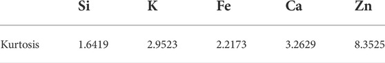
TABLE 1. First order differential distribution kurtosis values for the five substances.

From Table 1, it can be seen that the kurtosis of Si is the smallest, indicating that it has a wider distribution of the first-order differences, and the raw data show larger variation range of adjacent data and higher frequency of data mutation. Meanwhile, the kurtosis of Zn is the largest, followed by that of Ca, indicating that the distribution of the first-order differences in the raw data is narrower, with severe trailing, large values of outliers, and a large degree of peak-to-valley variation in some moments. These may explain the low correlation between the concentration data of suspended particulate matter and the Stokes data.

4.2 Discussion of training length and predicting length

In this section, we explored the appropriate training length and predicting length, and found out that the optimal training length is 3 days, while the optimal predicting length is 1 day. As shown in Figure 10A, we used MAPE between the predicted and measured value to evaluate the accuracy of the prediction results.

FIGURE 10

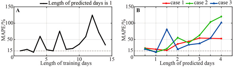
FIGURE 10. Exploring the optimal length of training and predicting. (A)shows the curve of MAPE between predicted and measured values as a function of training length; (B) shows the curve of MAPE between predicted and measured values as a function of predicting length under three predicting cases.

Figure 10A shows that the MAPE values for training lengths of 1, 3 and 6 days is smaller, around 15%, and the MAPE values will be larger for training lengths more than 7 days. Figure 10B shows the MAPE values of different predicting lengths. When discussing the optimal predicting length, there needs to be a restriction on the training length, and different training lengths may correspond to different optimal predicting lengths. Therefore, it is necessary to design the variation process of training length so that the final optimal predicting length obtained is universal. Three cases of training length and predicting length variation processes are designed:

Case 1:. The training length is constant at 8 days, and the prediction length starts at 0.5 day and increases with an interval of 0.5 day;

Case 2:. The training length is initially 1.5 days, and the prediction length is initially 0.5 day, keeping the training to prediction ratio constant at 3 and increasing the prediction length with an interval of 0.5 day;

Case 3:. The training length is initially 2 days, and the training length is incremented with an interval of 1 day, the prediction length is initially 0.5 day, and the prediction length is incremented with an interval of 0.5 dayFrom Figure 10B, when the predicting length is 0.5 and 1 day, the MAPE is generally lower. It also can be seen that the MAPE shows a rising trend after the predicting length exceeds 2 days. For an appropriate training length, the MAPE values are always less than 15%, when the predicting length is 1 day.

5 Conclusion

In this paper, for the first time we use multi-angle simultaneous polarization measurement data to predict the concentration of suspended particles in the outdoor atmosphere. The research starts from a correlation analysis. This paper first proposed a PCCA method to extract the correlation combination between the Stokes vectors and the concentration data of suspended particulate matter. Then, based on ARMA & LWLR method, we present how to predict the future trends of the concentration of suspended particulate matter. This paper also discussed the effect of the degree and frequency of data mutation on the correlation analysis, and investigated the optimal training length and prediction length. The studies show the optimal training length of 3 days and the optimal prediction length of 1 day.

Data availability statement

The original contributions presented in the study are included in the article/supplementary material, further inquiries can be directed to the corresponding author.

Author contributions

NZ, XY, and JS conceived the idea of the manuscript. XY and JS prepared the samples and processed the data. XY wrote the original manuscript and analyzed the results. NZ and HM performed the language editing. All authors contributed to the article and approved the submitted version.

Funding

This work is funded by Science and Technology Research Program of Shenzhen (JCYJ20200109142820687 and JCYJ20210324120012035) and the Cross-research innovation fund of International Graduate School at Shenzhen, Tsinghua University (JC2021002).

Acknowledgments

We thank the Shanghai Environmental Monitoring Center, Ministry of Ecology and Environment of the People’s Republic of China for their help.

Conflict of interest

The authors declare that the research was conducted in the absence of any commercial or financial relationships that could be construed as a potential conflict of interest.

Publisher’s note

All claims expressed in this article are solely those of the authors and do not necessarily represent those of their affiliated organizations, or those of the publisher, the editors and the reviewers. Any product that may be evaluated in this article, or claim that may be made by its manufacturer, is not guaranteed or endorsed by the publisher.

References

Ahmadianfar, I., Jamei, M., and Chu, X. (2020). A novel hybrid wavelet-locally weighted linear regression (W-lwlr) model for electrical conductivity (EC) prediction in surface water. J. Contam. Hydrol. 232, 103641. doi:10.1016/j.jconhyd.2020.103641

PubMed Abstract | CrossRef Full Text | Google Scholar

Berthet, G., Renard, J., Brogniez, C., Robert, C., Chartier, M., and Pirre, M. (2002). Optical and physical properties of stratospheric aerosols from balloon measurements in the visible and near-infrared domains I Analysis of aerosol extinction spectra from the AMON and SALOMON balloonborne spectrometers. Appl. Opt. 41 (36), 7522. doi:10.1364/ao.41.007522

PubMed Abstract | CrossRef Full Text | Google Scholar

Cleveland, W., and Devlin, S. (1988). Locally weighted regression: An approach to regression analysis by local fitting. J. Am. Stat. Assoc. 83 (403), 596–610. doi:10.1080/01621459.1988.10478639

CrossRef Full Text | Google Scholar

De Gooijer, J. G., and Hyndman, R. J. (2006). 25 years of time series forecasting. Int. J. Forecast. 22 (3), 443–473. doi:10.1016/j.ijforecast.2006.01.001

CrossRef Full Text | Google Scholar

Douwes, J., Thorne, P., Pearce, N., and Heederik, D. (2003). Bioaerosol health effects and exposure assessment: Progress and prospects. Ann. Occup. Hyg. 47 (3), 187–200. doi:10.1093/annhyg/meg032

PubMed Abstract | CrossRef Full Text | Google Scholar

Fowler, D., Coyle, M., Skiba, U., Sutton, M. A., Cape, J. N., Reis, S., et al. (2013). The global nitrogen cycle in the twenty-first century. Phil. Trans. R. Soc. B 368 (1621), 20130164. doi:10.1098/rstb.2013.0164

PubMed Abstract | CrossRef Full Text | Google Scholar

Gao, H., Yang, Y., Akampumuza, O., Hou, J., Zhang, H., and Qin, X. (2017). A low filtration resistance three-dimensional composite membrane fabricated via free surface electrospinning for effective PM2.5 capture. Environ. Sci. Nano 4 (4), 864–875. doi:10.1039/c6en00696e

CrossRef Full Text | Google Scholar

Gold, D. R., Litonjua, A., Schwartz, J., Lovett, E., Larson, A., Nearing, B., et al. (2000). Ambient pollution and heart rate variability. Circulation 101 (11), 1267–1273. doi:10.1161/01.cir.101.11.1267

PubMed Abstract | CrossRef Full Text | Google Scholar

Green, R., Sosik, H., Olson, R., and DuRand, M. (2003). Flow cytometric determination of size and complex refractive index for marine particles: Comparison with independent and bulk estimates. Appl. Opt. 42 (3), 526. doi:10.1364/ao.42.000526

PubMed Abstract | CrossRef Full Text | Google Scholar

Guaita, R., Pichiule, M., Mate, T., Linares, C., and Diaz, J. (2011). Short-term impact of particulate matter (PM(2.5)) on respiratory mortality in Madrid. Int. J. Environ. Health Res. 21 (4), 260–274. doi:10.1080/09603123.2010.544033

PubMed Abstract | CrossRef Full Text | Google Scholar

Guo, W., Zeng, N., Liao, R., Xu, Q., Guo, J., He, Y., et al. (2022). Simultaneous retrieval of aerosol size and composition by multi-angle polarization scattering measurements. Opt. Lasers Eng. 149, 106799. doi:10.1016/j.optlaseng.2021.106799

CrossRef Full Text | Google Scholar

Harrington, P. (2012). Machine learning in action. Manhattan, NY , USA: Shelter Island.

Google Scholar

Haywood, J., and Boucher, O. (2000). Estimates of the direct and indirect radiative forcing due to tropospheric aerosols: A review. Rev. Geophys. 38 (4), 513–543. doi:10.1029/1999rg000078

CrossRef Full Text | Google Scholar

Hotelling, H. (1936). Relations between two sets of variates. Biometrika 28 (3/4), 321–377. doi:10.2307/2333955

CrossRef Full Text | Google Scholar

Hu, J., Khan, F., Zhang, L., and Tian, S. (2020). Data-driven early warning model for screenout scenarios in shale gas fracturing operation. Comput. Chem. Eng. 143, 107116. doi:10.1016/j.compchemeng.2020.107116

CrossRef Full Text | Google Scholar

Huang, Z. Y., Lin, S., Long, L. L., Cao, J. Y., Luo, F., Qin, W. C., et al. (2020). Predicting the morbidity of chronic obstructive pulmonary disease based on multiple locally weighted linear regression model with K-means clustering. Int. J. Med. Inf. 139, 104141. doi:10.1016/j.ijmedinf.2020.104141

PubMed Abstract | CrossRef Full Text | Google Scholar

Li, D., Chen, F., Zeng, N., Qiu, Z., He, H., He, Y., et al. (2019). Study on polarization scattering applied in aerosol recognition in the air. Opt. Express 27 (12), A581–A595. doi:10.1364/OE.27.00A581

PubMed Abstract | CrossRef Full Text | Google Scholar

Mauderly, J., and Chow, J. (2008). Health effects of organic aerosols. Inhal. Toxicol. 20 (3), 257–288. doi:10.1080/08958370701866008

PubMed Abstract | CrossRef Full Text | Google Scholar

Miffre, A., David, G., Thomas, B., Rairoux, P., Fjaeraa, A. M., Kristiansen, N. I., et al. (2012). Volcanic aerosol optical properties and phase partitioning behavior after long-range advection characterized by UV-Lidar measurements. Atmos. Environ. 48, 76–84. doi:10.1016/j.atmosenv.2011.03.057

CrossRef Full Text | Google Scholar

Olin, J., and Sem, G. (1971). 1967Piezoelectric microbalance for monitoring the mass concentration of suspended particles. Atmos. Environ. 5 (8), 653–668. doi:10.1016/0004-6981(71)90123-5

CrossRef Full Text | Google Scholar

Patashnick, H., and Rupprecht, E. G. (2012). Continuous PM-10 measurements using the tapered element oscillating microbalance. J. Air & Waste Manag. Assoc. 41 (8), 1079–1083. doi:10.1080/10473289.1991.10466903

CrossRef Full Text | Google Scholar

Shang, D., Peng, J., Guo, S., Wu, Z., and Hu, M. (2020). Secondary aerosol formation in winter haze over the Beijing-Tianjin-Hebei Region, China. Front. Environ. Sci. Eng. 15 (2), 34. doi:10.1007/s11783-020-1326-x

CrossRef Full Text | Google Scholar

Suwa, T., Hogg, J., Quinlan, K., Ohgami, A., Vincent, R., and van Eeden, S. (2002). Particulate air pollution induces progression of atherosclerosis. J. Am. Coll. Cardiol. 39 (6), 935–942. doi:10.1016/s0735-1097(02)01715-1

PubMed Abstract | CrossRef Full Text | Google Scholar

Thomas, J., Jimenez-Aranda, A., Finlayson-Pitts, B., and Dabdub, D. (2007). Gas-Phase molecular halogen formation from NaCl and NaBr aerosols: When are interface reactions important? J. Phys. Chem. A 111 (30), 7243–7244. doi:10.1021/jp073927v

CrossRef Full Text | Google Scholar

Wang, J., Yu, L., Lai, K., and Zhang, X. (2016). Locally weighted linear regression for cross-lingual valence-arousal prediction of affective words. Neurocomputing 194, 271–278. doi:10.1016/j.neucom.2016.02.057

CrossRef Full Text | Google Scholar

Wang, S., Baxter, L., and Fonseca, F. (2008). Biomass fly ash in concrete: SEM, EDX and ESEM analysis. Fuel 87 (3), 372–379. doi:10.1016/j.fuel.2007.05.024

CrossRef Full Text | Google Scholar

Wellenius, G. A., Bateson, T. F., Mittleman, M. A., and Schwartz, J. (2005). Particulate air pollution and the rate of hospitalization for congestive heart failure among medicare beneficiaries in Pittsburgh, Pennsylvania. Am. J. Epidemiol. 161 (11), 1030–1036. doi:10.1093/aje/kwi135

PubMed Abstract | CrossRef Full Text | Google Scholar

Woźniak, S. B., Sagan, S., Zabłocka, M., Stoń-Egiert, J., and Borzycka, K. (2018). Light scattering and backscattering by particles suspended in the Baltic Sea in relation to the mass concentration of particles and the proportions of their organic and inorganic fractions. J. Mar. Syst. 182, 79–96. doi:10.1016/j.jmarsys.2017.12.005

CrossRef Full Text | Google Scholar

Xu, Q., Zeng, N., Guo, W., Guo, J., He, Y., and Ma, H. (2021). Real time and online aerosol identification based on deep learning of multi-angle synchronous polarization scattering indexes. Opt. Express 29 (12), 18540–18564. doi:10.1364/OE.426501

PubMed Abstract | CrossRef Full Text | Google Scholar

Xue, J., Li, Y., Quiros, D., Wang, X., Durbin, T., Johnson, K., et al. (2016). Using a new inversion matrix for a fast-sizing spectrometer and a photo-acoustic instrument to determine suspended particulate mass over a transient cycle for light-duty vehicles. Aerosol Sci. Technol. 50 (11), 1227–1238. doi:10.1080/02786826.2016.1239247

CrossRef Full Text | Google Scholar