Adaptive graph convolutional imputation network for environmental sensor data recovery

Environmental sensors are essential for tracking weather conditions and changing trends, thus preventing adverse effects on species and environment. Missing values are inevitable in sensor recordings due to equipment malfunctions and measurement errors. Recent representation learning methods attempt to reconstruct missing values by capturing the temporal dependencies of sensor signals as handling time series data. However, existing approaches fall short of simultaneously capturing spatio-temporal dependencies in the network and fail to explicitly model sensor relations in a data-driven manner. In this work, we propose a novel Adaptive Graph Convolutional Imputation Network for missing value imputation in environmental sensor networks. A bidirectional graph convolutional gated recurrent unit module is introduced to extract spatio-temporal features which takes full advantage of the available observations from the target sensor and its neighboring sensors to recover the missing values. In addition, we design an adaptive graph learning layer that learns a sensor network topology in an end-to-end framework, in which no prior network information is needed for capturing spatial dependencies. Extensive experiments on three real-world environmental sensor datasets (solar radiation, air quality, relative humidity) in both in-sample and out-of-sample settings demonstrate the superior performance of the proposed framework for completing missing values in the environmental sensor network, which could potentially support environmental monitoring and assessment.

1 Introduction

Environmental monitoring is essential for understanding our ecosystem and further preventing adverse effects on species and environment (Lanzolla and Spadavecchia, 2021). Wireless sensor networks (WSNs) facilitate innovative and pervasive environ-mental monitoring by providing a lot of significant benefits such as access to real time weather data, long-term monitoring, and broad area coverage (Ibrahim et al., 2021). Environmental sensor networks usually consist of a great number of distributed devices in different domains, and their usage has allowed for a variety of applications, such as urban noise control (Luo et al., 2020), plant health status monitoring (Di Nisio et al., 2020), coastal dune system study (Domínguez-Brito et al., 2020), and so forth.

Missing values widely exist in environmental sensor recordings due to many reasons, such as the malfunction of the devices, errors in signal transmission, power run out, and accidental manual system closure (Choi et al., 2021). These missing values in sensor signals can lead to several problems in the data processing and have a negative impact on sensor data analysis and data mining if they are not handled properly (Gruenwald et al., 2007). To deal with missing values, the most intuitive way is to remove all incomplete data samples and continue the analysis merely with the complete ones. Although this strategy efficiently simplifies the problem, lower sample size potentially leads to biased results and reduced study power, especially when the missing ratio of the dataset is large. In this context, developing more advanced methods to accurately impute the missing values is of great need and significance.

During the last decade, a series of deep learning techniques (LeCun et al., 2015; Schmidhuber, 2015; Goodfellow et al., 2016) have been explored in the imputation problem (Yoon et al., 2018b; Cao et al., 2018; Liu et al., 2019). The majority of this line of research adopts temporal imputation approaches which merely rely on temporal relations to complete the missing values of the time series. Specifically, the researchers leveraged past and future values near a missing point or block to reconstruct the missing parts in a dataset. As limited modifications on standard sequence models, these methods completely ignore valuable relational information between time series sequences (Chung et al., 2014; Vaswani et al., 2017; Bai et al., 2018).

More recently, a few approaches (Spinelli et al., 2020; Cini et al., 2021) incorporated graph structure to capture the spatial dependencies between signal sequences and leveraged the observations of neighboring sequences for missing value completion. These methods achieved considerable improvement on the imputation accuracy. The existing models completely rely on a predefined graph to capture shared patterns between signal sequences. However, the static graphs obtained in the heuristics manner are inherently corrupted, incomplete, and not adaptable to different sensor networks. Hence, how to generate a graph that fully captures the relation information and adaptively adjust to different environmental sensor networks is the research problem we are exploring in this work.

The limitations of existing methods dealing with missing value imputation can be summarized as follows. 1) Insufficient consideration of spatial dependencies. Most of the existing approaches built imputation models operating independently on the available data of each individual sensor, while the relation information and available observations of neighboring sensors are not fully leveraged. 2) Noisy and incomplete graph in the initialization. The majority of existing approaches generated a static graph based on a predefined distance operator. Graphs constructed using geographic distances can not fully capture the accurate relations thus hinder the model performance. 3) Fail to adaptively learn the graph structure. Few approaches that model spatial dependencies via graphs are primarily based on a predefined static graph, which can neither capture the dynamics nor generalize well to different sensor networks.

Motivated by these limitations, we propose a novel deep learning framework, called Adaptive Graph Convolutional Imputation Network (AGCIN), to simultaneously model the spatial and temporal dependencies for accurate and efficient missing value imputation in environmental sensor networks. To obtain a good initialization of the graph adjacency matrix, Canberra similarity function is performed on the incomplete dataset to capture the generic functional dependency between sensors in the latent space. The learned node embeddings obtained from the adaptive graph learning layer are incorporated with a global graph learning layer to generate the graph that captures the spatial dependencies between the environmental sensors in the network. Furthermore, we combine adaptive graph convolution with bidirectional recurrent networks and propose a new imputation framework, AGCIN, to model spatio-temporal dependencies in the sensor data recovery task. The major contributions of this work are as follows:

• Propose a novel and practical framework that exploits graph structure learning to solve the sensor data recovery problem. The proposed framework integrates adaptive graph convolution with bidirectional gated recurrent unit (GRU) network to capture spatio-temporal dependencies for imputing missing values.

• Design a strategy to generate an initial graph and learn a global adjacency matrix of the sensor network. This technique relies on node feature similarity and efficiently infers the posterior of the graph structure, even the geographic location information of the sensors is not available. The global adjacency matrix is obtained by masking the initialized graph with a learned matrix.

• Adaptively construct the graph that captures the spatial relations in the sensor network. We infer the underlying spatial dependencies that best fit the sensor data via learning node embeddings instead of conducting imputation with a predefined static graph in the imputation task. The corresponding edge weights in the adjacency matrix are optimized in the proposed end-to-end framework.

• Conduct extensive experiments on three real-world environmental sensor datasets. The proposed framework is evaluated on three environmental sensor networks with different data missing ratios. The proposed AGCIN outperforms state-of-the-art models in both in-sample and out-of-sample settings. Ablation study further demonstrates the effectiveness of different designed modules on improving imputation performance.

The remainder of the paper is organized as follows. Section 2 reviews the literature on missing value imputation, especially in the context of deep learning techniques and the emergence of graph neural networks. Section 3 describes the preliminary concept and problem formulation, and is followed by a detailed introduction of AGCIN in Section 4. The empirical evaluations are presented in Section 5. Finally, Section 6 concludes the work.

2 Related work

A large literature exists on the topic of missing value imputation, and most of the approaches are based on standard time series forecasting methods and similarity operators. A basic method is the mean approach which intuitively replaces the missing points with the average of the observed values. K-nearest neighbors (KNN) has also been widely implemented to impute missing values in a sensor network (Troyanskaya et al., 2001; Beretta and Santaniello, 2016), in which the missing parts of a certain sensor is filled by averaging or weighting the values of its closest k neighbors. Other popular alternatives include the expectation-maximization (EM) algorithm (Ghahramani and Jordan, 1993; Nelwamondo et al., 2007), linear methods (Yi et al., 2016), state-space models (Durbin and Koopman, 2012; Walter et al., 2013), ensemble learning methods (Stekhoven and Bühlmann, 2012; Ding et al., 2019), and low-rank approximation methods (Cichocki and Phan, 2009; Cai et al., 2010; Rao et al., 2015; Yu et al., 2016; Mei et al., 2017).

Recently, deep learning techniques have dominated a relevant task, time series forecasting, due to its superior power to learn complex dependencies in an end-to-end manner. More deep neural networks emerge in the topic of time series imputation. Among them, deep autoregressive methods and recurrent neural networks (RNNs) achieve success in regards to its exceptional power to model sequential data (Lipton et al., 2016; Yoon et al., 2018b; Cao et al., 2018; Che et al., 2018; Luo et al., 2018). Che et al. (2018) proposed GRU-D which designed a decay mechanism of the hidden states of GRU to process sequences with missing data. BRITS (Cao et al., 2018), similar to a bidirectional structure of GRU-D, was designed for multivariate time series imputation, in which the correlation among different channels was taken into consideration. Inspired by the idea that missing parts can be imputed by sampling from the distribution of available data, deep latent variable approaches are explored in the imputation task (Rezende et al., 2014; Ma et al., 2018a; Ma et al., 2018b; Mattei and Frellsen, 2018; Mattei and Frellsen, 2019; Nazabal et al., 2020). Specifically, Rezende et al. (2014) estimated the conditional distribution of missing values based on the observed distribution. Then, sampling is conducted by a Markov chain to perform data denoising and imputation. Mattei and Frellsen (2018) extended the approach by improving the sampling strategy with Metropolis-within-Gibbs sampling. The weaknesses of these methods are that the researchers assume missing data patterns are missing-at-random (MAR) and the entire dataset is available (Rubin, 1976). To handle the presence of missing values, other deep latent variable models are proposed, including p-VAE (Ma et al., 2018a; Ma et al., 2018b) that incorporated a permutation invariant encoder and VAE lower bound, MIWAE (Mattei and Frellsen, 2019) that extended the importance-weighted autoencoder lower bound (Burda et al., 2015), and HI-VAE (Nazabal et al., 2020) that leveraged an extension of the variational autoencoder lower bound. Above deep latent variable models are based on strong assumptions of certain data missingness patterns. However, the assumptions are too strong to be fitted in real-world scenarios.

More recently, adversarial training strategy has been incorporated to generate realistic reconstructed times series (Yoon et al., 2018a; Luo et al., 2018; Luo et al., 2019; Richardson et al., 2020; Miao et al., 2021; Qin et al., 2021). Specifically, Yoon et al. (2018a) proposed GAIN to perform missing value imputation in the i.i.d. settings under a generative adversarial network (GAN) (Goodfellow et al., 2014). Different from the prior research, Luo et al. (2018), (2019) designed deep generative models to generate realistic synthetic sequences to replace the missing values. Along the same line of research, Richardson et al. (2020) developed a training strategy to train a normalizing flow and a deterministic inference network simultaneously for missing data completion. Although such an inference network can generate deterministic inferences along with the distributions learned by a normalizing flow, it fails to stochastically sample from the conditional distributions given by the flow. Miao et al. (2021) proposed a conditional generator on predicted labels for the target time series. These aforementioned methods primarily rely on modifications of standard neural architectures tailored for modeling temporal dependencies, while relational information between time series has not been explored. To capture the complex spatio-temporal patterns in traffic data imputation, Qin et al. (2021) designed a temporal graph convolutional variational autoencoder, which introduced a self-interested coalitional learning (SCL) strategy by leveraging the cooperation and competition with an additional discriminator. Due to its strong dependence on the temporal characteristics of the dataset, this approach is merely designed for the data imputation under intermittent missing pattern setting but not for the persistent missing pattern setting.

With their advantages to model spatial dependencies, graph neural networks (GNNs) have achieved great success in spatio-temporal forecasting (Li et al., 2017; Yu et al., 2017; Seo et al., 2018; Zhang et al., 2018; Cai et al., 2020). Most of the methods modified standard RNNs by incorporating graph convolutional layers. Seo et al. (2018) proposed a type of GRU cell, in which both update and reset gates are updated by GNNs in the spectral domain (Defferrard et al., 2016). Li et al. (2017) developed a similar framework which utilized a diffusion convolution operator (Atwood and Towsley, 2016) instead of spectral GNNs. Some other approaches (Yu et al., 2017; Wu et al., 2019, 2020) explored the switching convolutions on spatial and temporal dimensions. Attention-based spatio-temporal prediction methods (Vaswani et al., 2017; Zhang et al., 2018; Cai et al., 2020) enabled the models to automatically focus on the most relevant parts in the sequence data thus enhancing the predictive performance. Recently, graph structure learning models (Kipf et al., 2018; Wu et al., 2020; Shang et al., 2021) that attract the research attention in spatio-temporal forecasting problems, along with the relevant problem of evolving graph topology (Zambon et al., 2019; Paassen et al., 2020), provide a data-driven approach to improve the quality of graph and learn informative node representations.

Surprisingly, GNNs are not fully explored in the missing value imputation problem. Among the few that use graphs to capture the spatial dependencies, Spinelli et al. (2020) proposed an adversarial approach to train GNNs for imputing missing data, and You et al. (2020) developed a bipartite graph representation learning network for node feature completion. Kuppannagari et al. (2021) proposed a graph-based denoising autoencoder for spatio-temporal data coming from smart grids with known topology. With the consideration of relational aspects in the imputation task, Cini et al. (2021) designed a graph recurrent imputation network for reconstructing missing values in generic multivariate time series. However, we argue that none of the aforementioned approaches take full advantage of flexible graph structure learning since they merely rely on a predefined graph to model the spatial dependencies. The primary goal of this work is to explore the feasibility of an adaptive graph learning strategy that generalizes to varied sensor networks to enhance missing data inference and imputation.

3 Problem formulation

This paper aims to propose a framework to reconstruct missing values in the environmental sensor networks. The related concept and problem formulation are presented in this section.

3.1 Sensor network

The topological structure of a sensor network is modeled as a weighted, undirected graph ${\mathcal{G}}_t$ with the fixed number of N nodes at each time step t. A graph is composed of node features X_t and adjacency matrix A_t, where ${\mathbf{X}}_t\in {\mathbb{R}}^{N\times d}$ presents the node feature matrix, and entry $a_t^{i,j}$ of the adjacency matrix ${\mathit{A}}_t\in {\mathbb{R}}^{N\times N}$ denotes the scalar weight of the edge between a pair of nodes i and j. As we focus on graph structure learning in this work, we assume the topology of the graph is refined by time step during model training, i.e., at each time step, A_t ≠ A_t−1.

3.2 Sensor data recovery

To model the data missing patterns, we define a binary mask M_t ∈ {0,1}^N×c where each row ${\mathbf{m}}_t^i$ denotes the missingness condition of node features of ${\mathbf{x}}_t^i$ in X_t. Specifically, ${\mathbf{m}}_t^{i,j}=0$ implies the features are missing, while ${\mathbf{m}}_t^{i,j}=1$ indicates that ${\mathbf{x}}_t^{i,j}$ is available, then the actual value of sensor recording is stored in ${\mathbf{x}}_t^{i,j}$.

The sensor data recovery problem can be formally defined as: given a sensor network with signal time series ${\mathcal{G}}_{[t,t+T]}$ of a window size of T, we can define the missing data completion error as:

$\begin{array}{cc}\hfill & \mathcal{L}\left(\widehat{{\mathbf{X}}_{ }^{ }}{\mathbf{ }}_{\left[t,t+T\right]},{\mathbf{X}}_{\left[t,t+T\right]},{\bar{\mathbf{M}}}_{\left[t,t+T\right]}\right)\hfill \\ \hfill & =\sum _{h=t}^{t+T}\sum _{i=1}^N\frac{{\bar{\mathbf{m}}}_h^i\cdot \ell \left(\widehat{{\mathbf{x}}_{ }^{ }}{ }_h^i,{\mathbf{x}}_h^i\right)}{{\bar{\mathbf{m}}}_h^i\cdot {\bar{\mathbf{m}}}_h^i},\hfill \end{array}(1)$

where $\widehat{{\mathbf{X}}_t^{ }}$ and ${\mathbf{X}}_t$ denote the node feature matrix after imputation and ground truth node feature matrix without any missing data, respectively. $\widehat{{\mathbf{x}}_{ }^{ }}{ }_h^i$ is the reconstructed ${\mathbf{x}}_h^i;{\bar{\mathbf{M}}}_{[t,t+T]}$ and ${\bar{\mathbf{m}}}_h^i$ are the logical binary complement of M_[t,t+T] and ${\mathbf{m}}_h^i$, respectively. ℓ(⋅, ⋅) denotes the element-wise error function.

To design a parametric and trainable imputation model, two different operational settings are discussed. In the in-sample imputation setting, the model is trained to complete missing values in an input sequence X_[t,t+T] of a given fixed length T. To be specific, all the available data can be used to train the model except missing values and those that have been removed from the sequence for failure check. In the second setting, the model is trained and evaluated on disjoint sequences under the out-of-sample case. It is worth mentioning that the model has no access to the ground truth data removed out from the original data for the final evaluation in both settings.

4 Methodology

The overall framework of the proposed AGCIN is presented in Figure 1. The graph structure learning module incorporates the initial graph and node embeddings to reconstruct the adjacency matrix, which is then used as an input to all graph convolution layers. To simultaneously model spatial and temporal dependencies, graph convolution layers are incorporated with bidirectional GRU. In more detail, the core components of our framework are detailed in the following.

FIGURE 1

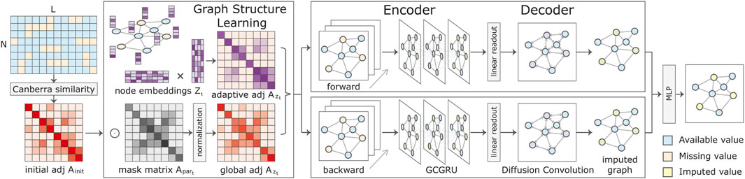
FIGURE 1. Model architecture of the proposed Adaptive Graph Convolutional Imputation Network (AGCIN). The initial adjacency matrix is obtained by computing the pair-wise Canberra similarity of the sensor sequences. The graph structure learning module refines the learned graph topology by combining global and adaptive adjacency matrices. Each of the forward and backward imputation modules is composed of an encoder and a decoder. The encoder sequentially processes the input sequences with missing values to obtain the hidden node representations. In the decoder, the first-stage imputation is performed through a linear readout function, and the spatial decoder refines imputed values in the second stage. The final imputations are obtained through an MLP aggregating the forward and backward learned node representations.

4.1 Graph structure learning

As the node embeddings are computed by recursively aggregating information from neighboring nodes, the adjacency matrix is important to GNNs. Different from prior approaches in the imputation task, we construct the adjacency matrix based on two learners, one for global adjacency matrix, and the other for adaptive adjacency matrix. The motivation of designing these two learners is that the first learner introduces prior pair-wise similarity relations of the sensors, making the training start from a good initialization; the second learner is intended to refine the graph structure based on the node embeddings learned during the training process.

4.1.1 Global adjacency matrix

To capture the underlying relations of the sensors, instead of the geographic locations, we generate the initial graph from node features. As a classical numerical measure of the distance between pairs of points in the vector space, Canberra distance (Androutsos et al., 1998) is adopted as the similarity function to build the initial graph adjacency matrix. The Canberra distance between signal sequences of a sensor pair i and j is defined as follows:

$\mathrm{C}\mathrm{d}\mathrm{i}\mathrm{s}\mathrm{t}\left({\mathbf{x}}^i,{\mathbf{x}}^j\right)=\sum _n\frac{\left|{\mathbf{x}}_n^i-{\mathbf{x}}_n^j\right|}{\left|{\mathbf{x}}_n^i\right|+\left|{\mathbf{x}}_n^j\right|},(2)$

where ${\mathbf{x}}^i=({\mathbf{x}}_1^i,{\mathbf{x}}_2^i,\dots ,{\mathbf{x}}_n^i)$ and ${\mathbf{x}}^j=({\mathbf{x}}_1^j,{\mathbf{x}}_2^j,\dots ,{\mathbf{x}}_n^j)$ are node feature vectors. We normalize Canberra distance by the length of non-missing part of the signal sequence pair, and obtain each element in the initial adjacency matrix A_init as follows:

$a_{\text{init}}^{i,j}=\left\{\begin{array}{cc}\hfill 1-\frac{\mathrm{C}\mathrm{d}\mathrm{i}\mathrm{s}\mathrm{t}\left({\mathbf{x}}^i,{\mathbf{x}}^j\right)}{n}\hfill & n>0\hfill \\ \hfill 0\hfill & \text{otherwise},\hfill \end{array}\right.(3)$

where n is the sequence length observed for both of the sensor pair. The range of the weight in the generated initial adjacency matrix is between 0 and 1, where 1 means the two vectors are exactly the same, and 0 indicates the maximum dissimilarity or the vector pair has no overlapping signal sequence available.

The global adjacency matrix learner utilizes the masking method to generate the new adjacency matrix by ${\mathbf{A}}_{m_t}={\mathbf{A}}_{{\text{par}}_t}\odot {\mathbf{A}}_{\text{init}}$, where ${\mathbf{A}}_{{\text{par}}_t}\in {\mathbb{R}}^{N\times N}$ is a trainable parameter matrix, ⊙ is the Hadamard product. An issue would occur to ${\mathbf{A}}_{m_t}$ that the weights in the position of zero values in the A_init are omitted. A scaled 1-hop residual is designed to address this issue. The global adjacency matrix is generated as follows:

$\begin{array}{cc}\hfill {\mathbf{D}}_{{m_t}^{ii}}& =\sum _j{\mathbf{A}}_{{m_t}^{ij}},i,j=1,\dots ,N\hfill \\ \hfill {\mathbf{D}}_{m_t}& =\mathrm{diag}\left(1/\left({\mathbf{D}}_{{m_t}^{ii}}+0.0001\right)\right),i=1,\dots ,N\hfill \\ \hfill {\mathbf{A}}_{g_t}& ={\mathbf{D}}_{m_t}{\mathbf{A}}_{m_t},\hfill \end{array}$

where ${\mathbf{D}}_{{m_t}^{ii}}$ denotes the degree of node i, and ${\mathbf{D}}_{m_t}$ is the inverse matrix of degree matrix with a plus of 0.0001 to deal with the NaN problem, and ${\mathbf{A}}_{g_t}$ is the learned global adjacency matrix.

4.1.2 Adaptive adjacency matrix

To construct the adaptive adjacency matrix, we introduce an embedding vector for each sensor. Those embeddings are initialized randomly and then updated along with the other parameters during training, which are used for graph structure learning to capture the relations of sensors in the latent space. The reconstructed graph is obtained by the inner product of node embeddings as follows:

${\mathbf{A}}_{z_t}=\sigma \left({\mathbf{Z}}_t{\mathbf{Z}}_t^{\top }\right),(4)$

where ${\mathbf{Z}}_t\in {\mathbb{R}}^{N\times d}$ denotes node embeddings, and σ is the activation function, and the Relu function is adopted here. We aim to reconstruct the normalized adjacency matrix instead of the raw one, and this strategy can save considerate computational cost.

The final learned adjacency matrix is a weighted sum of the global and adaptive adjacency matrices. Motivated by the observation that real-world graphs have noisy, task-irrelevant edges, we usually enforce a sparsity constraint on the adjacency matrix. Instead of directly panelizing the non-zero entries, we implicitly sparsify the adjacency matrix by filtering out the smaller weights. In the module design, we use 0.75 quantile of the learned weights as a threshold. The graph obtained in the graph structure learning module is presented as follows:

${\mathbf{A}}_t=\text{ø}\left(\lambda {\mathbf{A}}_{z_t}+\left(1-\lambda \right){\mathbf{A}}_{g_t}\right),(5)$

where ø is the quantile filtering operator. This adaptive adjacency matrix is learned end-to-end through stochastic gradient descent.

4.2 Imputation module

The imputation module that replaces the missing values with estimated ones is composed of encoding and decoding stages.

4.2.1 Encoder

In the encoding stage, the input signal sequence X_[t,t+T] and mask M_[t,t+T] are handled sequentially by a GRU neural network with the gates updated by graph convolution layers. In principle, any graph convolution operator could be used. For the computational benefits, we adopt diffusion convolution (Atwood and Towsley, 2016) as the implementation of graph convolution layer in this work.

In particular, given the node feature vectors X_t with K orders of a predefined adjacency matrix, the graph convolution operator is described as:

$\mathbf{Z}=\sum _{K=0}^K{\mathbf{P}}^k\mathbf{X}{\mathbf{W}}_k,(6)$

where P^k denotes the power series of the transition matrix. In the case of an undirected graph, P = A/rowsumA. In this work, we propose an adaptive adjacency matrix A_t generated in Eq. 5. The adaptive graph convolution used for updating GRU gates is defined as follows:

$\mathrm{G}\mathrm{C}\left({\mathbf{X}}_t,{\mathbf{A}}_t\right)=\sum _{K=0}^K{\mathbf{A}}_t^k{\mathbf{X}}_t{\mathbf{W}}_k.(7)$

Note that several definitions of neighborhood are possible, e.g., one might consider nodes connected by paths up to a certain length l. For the sake of simplicity, from now on we use $\mathrm{G}\mathrm{C}\left({\mathbf{X}}_t,{\mathbf{A}}_t\right)$ to represent the forward pass of a K-layer graph convolutional neural network. Graph convolution is then utilized as the building blocks to extract spatio-temporal features. As implemented in previous approaches (Li et al., 2017; Seo et al., 2018), we adopt a GCGRU architecutre of incorporating the graph convolution layer defined above into GRU gates. The gate updating of GCGRU can be presented as:

$\begin{array}{cc}\hfill {\mathbf{r}}_t& =\sigma \left(\mathrm{G}\mathrm{C}\left(\left[\widehat{{\mathbf{x}}_{ }^{ }}{ }_t^{″},{\mathbf{m}}_t,{\mathbf{h}}_{t-1}\right],{\mathbf{A}}_t\right)\right),\hfill \\ \hfill {\mathbf{u}}_t& =\sigma \left(\mathrm{G}\mathrm{C}\left(\left[\widehat{{\mathbf{x}}_{ }^{ }}{ }_t^{″},{\mathbf{m}}_t,{\mathbf{h}}_{t-1}\right],{\mathbf{A}}_t\right)\right),\hfill \\ \hfill {\mathbf{c}}_t& =\tanh \left(\mathrm{G}\mathrm{C}\left(\left[\widehat{{\mathbf{x}}_{ }^{ }}{ }_t^{″},{\mathbf{m}}_t,{\mathbf{r}}_t\odot {\mathbf{h}}_{t-1}\right],{\mathbf{A}}_t\right)\right),\hfill \\ \hfill {\mathbf{h}}_t& ={\mathbf{u}}_t\odot {\mathbf{h}}_{t-1}+\left(1-{\mathbf{u}}_t\right)\odot {\mathbf{c}}_t,\hfill \end{array}$

where r_t, u_t are respectively the reset and update gates, h_t denotes the hidden node representations at time t, and the decoding block at the previous time step obtains the output $\widehat{{\mathbf{x}}_{ }^{ }}{ }_t^{″}$, which is discussed in the Decoder subsection. It is worthy of mentioning that for the time steps where input sequences contain missing values, predictions obtained from the decoder block is fed to the encoder. The output of the encoder module is the encoded sensor signal sequence H_[t,t+T].

4.2.2 Decoder

In the decoding stage, we first obtain one-step-ahead predictions via the hidden node representations of the GCGRU through a linear readout function as:

$\widehat{{\mathbf{Y}}_t^{\prime }}={\mathbf{H}}_{t-1}{\mathbf{V}}_h+{\mathbf{b}}_h,(8)$

where ${\mathbf{V}}_h\in {\mathbb{R}}^{l\times d}$ is a learnable adjacency matrix and ${\mathbf{b}}_h\in {\mathbb{R}}^d$ is a learnable vector on bias. The imputation operator is defined as follows:

$\mathrm{\Psi }\left({\mathbf{Y}}_t\right)={\mathbf{M}}_t\odot {\mathbf{X}}_t+{\bar{\mathbf{M}}}_t\odot {\mathbf{Y}}_t,(9)$

where Ψ denotes the imputation function. The missing data in input X_t is imputed with the values in Y_t at the same position. Through filling $\widehat{{\mathbf{Y}}_{ }^{ }}{ }_t^{\prime }$ to the imputation function, the read-out imputation $\widehat{{\mathbf{X}}_{ }^{ }}{ }_t^{\prime }$ is obtained and the output is X_t with missing data filled up by the one-step-ahead predictive values $\widehat{{\mathbf{Y}}_{ }^{ }}{ }_t^{\prime }$. Then, we concatenate the predictions, the mask M_t, and the hidden representation H_t−1, along with the adaptive graph A_t at time t, then process them with a diffusion convolution operator which obtains the imputation representation g_t as follows:

${\mathbf{g}}_t=\mathrm{G}\mathrm{C}\left(\left[\mathrm{\Psi }\left(\widehat{{\mathbf{x}}_{ }^{ }}{ }_t^{\prime }\right),{\mathbf{m}}_t,{\mathbf{h}}_{t-1}\right],{\mathbf{A}}_t\right).(10)$

As mentioned before, a node imputation representation merely depends on graph convolution calculated based on neighboring nodes and the representation at the previous step. As the next steps, we concatenate imputation representation G_t with hidden representation H_t−1, generate imputations for one more time via a linear readout function, and apply the imputation operator as:

$\begin{array}{c}\hfill \widehat{{\mathbf{Y}}_t^{″}}=\left[{\mathbf{G}}_t,{\mathbf{H}}_{t-1}\right]{\mathbf{V}}_g+{\mathbf{b}}_g,\end{array}(11)$

$\begin{array}{c}\hfill \widehat{{\mathbf{X}}_t^{″}}=\mathrm{\Psi }\left(\widehat{{\mathbf{Y}}_t^{″}}\right).\end{array}(12)$

Finally, we feed $\widehat{{\mathbf{X}}_t^{″}}$ as input to the GCGRU to update the hidden representations and proceed to process the next input sequences and learned adjacency matrix.

4.3 Bidirectional gated recurrent unit

Extending the imputation module to model forward and backward dynamics simultaneously can be achieved by duplicating the architecture described in Section 4.1 and Section 4.2. The first paralleled module processes the input sequence in the forward direction (from the beginning of the sequence towards its end), while the second one in the other way around. The final imputation of each node is obtained with an MLP aggregating representations extracted from the two directions as:

$\begin{array}{c}\hfill \widehat{{\mathbf{y}}_t^{ }}=MLP\left(\left[{\mathbf{g}}_t^{fwd},{\mathbf{h}}_{t-1}^{fwd},{\mathbf{g}}_t^{bwd},{\mathbf{h}}_{t+1}^{bwd}\right]\right).\end{array}(13)$

Then we can obtain the final imputations in the sensor network as:

$\widehat{{\mathbf{X}}_{ }^{ }}{\mathbf{ }}_{\left[t,t+T\right]}=\mathrm{\Psi }\left(\widehat{{\mathbf{Y}}_{ }^{ }},{\mathbf{ }}_{\left[t,t+T\right]}\right).(14)$

4.4 Loss function

It is important to realize that our model does not merely reconstruct the input as an autoencoder, but it is specifically tailored for the imputation task due to its inductive biases. The model is trained by minimizing the reconstruction error of all imputation stages in both directions. The objective of the proposed AGCIN is to learn the parameters by minimizing the error between the ground truth and imputed values. The loss function is defined as:

$\begin{array}{cc}\hfill \mathcal{L}& =\mathcal{L}\left(\widehat{{\mathbf{X}}_{ }^{ }}{\mathbf{ }}_{\left[t,t+T\right]},{\mathbf{X}}_{\left[t,t+T\right]},{\bar{\mathbf{M}}}_{\left[t,t+T\right]}\right)\hfill \\ \hfill & +\mathcal{L}\left(\widehat{{\mathbf{X}}_{ }^{ }}{ }_{\left[t,t+T\right]}^{\text{′}fwd},{\mathbf{X}}_{\left[t,t+T\right]},{\bar{\mathbf{M}}}_{\left[t,t+T\right]}\right)\hfill \\ \hfill & +\mathcal{L}\left(\widehat{{\mathbf{X}}_{ }^{ }}{ }_{\left[t,t+T\right]}^{\text{′}bwd},{\mathbf{X}}_{\left[t,t+T\right]},{\bar{\mathbf{M}}}_{\left[t,t+T\right]}\right)\hfill \\ \hfill & +\mathcal{L}\left(\widehat{{\mathbf{X}}_{ }^{ }}{ }_{\left[t,t+T\right]}^{\text{″}fwd},{\mathbf{X}}_{\left[t,t+T\right]},{\bar{\mathbf{M}}}_{\left[t,t+T\right]}\right)\hfill \\ \hfill & +\mathcal{L}\left(\widehat{{\mathbf{X}}_{ }^{ }}{ }_{\left[t,t+T\right]}^{\text{″}bwd},{\mathbf{X}}_{\left[t,t+T\right]},{\bar{\mathbf{M}}}_{\left[t,t+T\right]}\right),\hfill \end{array}(15)$

where each $\mathcal{L}(\cdot ,\cdot ,\cdot )$ can be obtained via Eq. 1 and we choose mean absolute error as the error function.

5 Experiments

The proposed framework is evaluated on three real-world environmental sensor datasets. Followed by the experimental setup in Section 5.1, a comparison of the imputation performance of AGCIN with state-of-the-art models and an analysis of the varied choices of embedding dimensions to construct the adaptive graph are conducted in Section 5.2 and Section 5.3, respectively. The results of an ablation study of the important modules in AGCIN are discussed in Section 5.4. To study the robustness of the proposed framework, Section 5.5 performs an assessment of model performance degradation under varied data missingness ratios. Section 5.6 presents a case study on the learned adjacency matrix with the visualization of imputation results from three environmental sensors with high weights in the learned adaptive adjacency matrix.

5.1 Experiment settings

5.1.1 Datasets

Three sensor networks that measure the air quality and other environmental conditions are used to empirically evaluate the proposed AGCIN.

• Radiation: a dataset that we aggregated on the recordings of 561 solar radiation sensors across the five regions (South, Southeast, North, Northeast, Central-West) of Brazil for the year of 2019. The sensing unit is Watt-hours per square meter (Wh/m²).

• PM2.5: a dataset on the PM2.5 pollutants (μg/m₃) of air quality indices recorded by 437 monitoring stations across 43 cities in China from 2014/5/1 to 2015/4/30.

• Humidity: a dataset that we combined the signals of 580 humidity sensors throughout Brazil that report relative humidity in % from 2018/1/1 to 2018/12/31.

All the datasets have more than 10% data missing, among which the imputation on air quality sensors is the most challenging with 25.67% recordings of PM2.5 pollutants missing. The summary statistics of three datasets are provided in Table 1.

TABLE 1

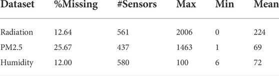
TABLE 1. Description of three datasets.

5.1.2 Comparison methods

The following methods are included in the performance comparison: 1) MEAN, a basic imputation approach based on the node-level average. 2) KNN, k-nearest neighbors algorithm that averages features of the k neighboring nodes with the highest weights in the adjacency matrix; 3) MF (Candès and Recht, 2009), matrix factorization method for completing missing values in a matrix assumed to contain redundancies and correlations. 4) MICE (White et al., 2011), a multiple imputation method used to impute missing values in a dataset under certain assumptions about the data missingness patterns. 5) MissForest (Stekhoven and Bühlmann, 2012), an ensemble imputation method based on random forests which averages over multiple unpruned regression trees. 6) MIWAE (Mattei and Frellsen, 2019), a deep latent variable model based on the importance-weighted autoencoder to handle missing values by maximizing a potentially tighter lower bound of the log-likelihood. 7) VAR (Lütkepohl, 2013), vector autoregressive is a statistical model used to capture the relationship between multiple quantities as they change over time. 8) GAIN, a revised version of missing data imputation (Yoon et al., 2018a) with bidirectional recurrent encoder and decoder, also can be seen as an unsupervised version of SSGAN (Miao et al., 2021). 9) BRITS (Cao et al., 2018), a bidirectional GRU model with decay mechanism of the hidden states of gated recurrent unit to process sequences with missing values. 10) GRIN (Cini et al., 2021), a graph neural network architecture that leverages message passing to learn spatio-temporal representations.

5.1.3 Settings and evaluation metrics

For the three datasets, we adopted the same evaluation protocol of previous works (Cao et al., 2018; Cini et al., 2021) and presented results for both the in-sample and out-of-sample settings (except for MF which only works in-sample). The diffusion convolution (Atwood and Towsley, 2016) was adopted for all the experiments. The window size T = 24 was set for all the datasets in line with (Cao et al., 2018; Cini et al., 2021). We separated the datasets to 7:2:1 for training, testing, validation, respectively. The hyperparameter λ in Eq. 5 was studied in the range of 0.1 to 0.9 with an interval of 0.1, and 0.7 was set for running AGCIN on all three datasets. We conducted all the experiments on a single 24 GB NVIDIA 3090 GPU.

For baseline models that leverages a predefined graph, we used the adjacency matrix obtained by thresholded Gaussian kernel (Shuman et al., 2013) computed from pair-wise geographic distance. The edge weight of a node pair i and j is defined as:

$a^{i,j}=\left\{\begin{array}{cc}\hfill \exp \left(-\frac{\mathrm{d}{\left(i,j\right)}^2}{\gamma }\right)\hfill & \mathrm{d}\left(i,j\right)\le \delta \hfill \\ \hfill 0\hfill & \text{\hspace{0.17em}otherwise\hspace{0.17em}},\hfill \end{array}\right.$

where d (⋅, ⋅) is the distance operator, γ controls the width of the kernel, and δ denotes the threshold. γ is set to the standard deviation of geographic distance.

We evaluated the sensor data imputation performance in terms of three metrics: mean absolute error (MAE), mean relative error (MRE) (Cao et al., 2018), and mean squared error (MSE).

5.2 Performance

The imputation results of the proposed AGCIN and baseline methods across the three datasets are tabulated in Table 2. In the in-sample setting, the metrics are computed on imputations obtained by averaging predictions over all the overlapping windows, while in the out-of-sample setting, the results of averaging the error over window length are reported. A comparative assessment of the results in both the in-sample and out-of-sample settings leads to the following observations: 1) The majority of the traditional methods (i.e., Mean, KNN, MF, and MICE) fail to achieve good imputation performance on the three datasets. MissForest achieves more accurate predictive results compared to the other methods, especially in the humidity dataset. 2) Deep learning models including MIWAE, VAR, GAIN, BRITS, generally achieve competitive performance, which emphasizes the importance of the temporal features in environmental sensor network imputation. Across the three datasets, BRITS achieves better imputation performance compared to VAR and GAIN models. The results obtained by BRITS in the humidity dataset are very competitive, which benefit from the modeling of underlying nonlinear dynamics via bidirectional LSTM with the temporal decay mechanism. Comparatively, MIWAE achieves low imputation accuracy, perhaps due to not all the assumptions fitted in the data missing scenarios. 3) The GNN-based models GRIN and AGCIN achieve large improvements in the imputation performance by incorporating the graph convolution operator to model the spatial dependencies. Capturing the spatial dependencies via graph convolution layers can greatly enhance the imputation accuracy. 4) Overall, the proposed AGCIN achieves the best performance across the evaluation metrics for all three datasets. The results demonstrate that the proposed framework to learn graph structure from data can more accurately model the spatial and temporal dependencies in the environmental sensor networks and achieve promising imputation results. The performance enhancements from AGCIN that adaptively generates graph over state-of-the-art method GRIN which uses a fixed predefined graph are 4.4%, 5.6%, and 9.77% on radiation, PM2.5, humidity datasets, respectively.

TABLE 2

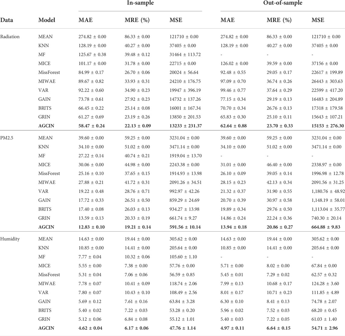
TABLE 2. Imputation performance comparison of the proposed AGCIN and baseline methods.

5.3 Embedding dimension

The dimension of node embeddings potentially has an impact on the quality of learned graph, and it is one of the important hyperparameters in our framework. Figure 2 plots the influence of choosing different embedding dimensions for AGCIN on the three datasets. Generally, good performance is achieved across all the tested embedding dimensions, especially the comparative higher dimensions. Also, it is observed that high embedding dimensions exceeding a certain value do not necessarily bring better imputation performance. A higher node embedding dimension increases the number of parameters updated during training, which makes the model take more time to optimize, and even worse, result in the over-fitting issue. A suitable node embedding dimension is supposed to find a balance between the ability to learn rich node representation and the number of model parameters. Within the tested node embedding dimensions {4, 8, 12, 16, 24, 32}, the appropriate node embedding dimension across the datasets is 16. A higher node embedding dimension, such as 24 or 32, potentially results in slightly better imputation performance but that improvement is negligible. The highest tested embedding dimension as 32 on PM2.5 dataset results in performance degradation.

FIGURE 2

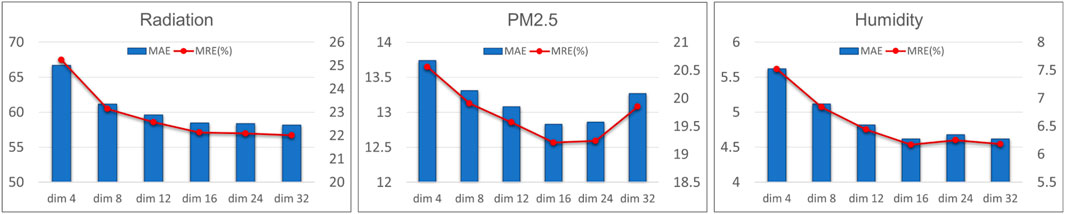
FIGURE 2. Study of varied embedding dimensions for constructing adaptive graphs on three datasets.

5.4 Ablation study

To evaluate the importance of the different designed modules, we conducted an ablation study on AGCIN by selectively instantiating varied model framework configurations on PM2.5 dataset and reporting the performance metrics in Table 3. We compared the performance of the originally designed version with the variants that remove certain components in orders, including global adjacency matrix learner introduced in Section 4.1.1, adaptive adjacency matrix learner in Section 4.1.2, spatial decoder in Section 4.2.2, and bidirectional architecture of GCGRU in Section 4.3, respectively. Ablation testing results demonstrate that each of the modules has a positive impact on the final imputations. Specifically, the imputation accuracy can be greatly enhanced by adopting the proposed adaptive graph learning strategy even without an initial graph fed into the graph convolution operation. Additionally, the full version of AGCIN improves the imputation performance of the base model by 13.3% in MAE, 13.19% in MRE, and 22.67% in MSE.

TABLE 3

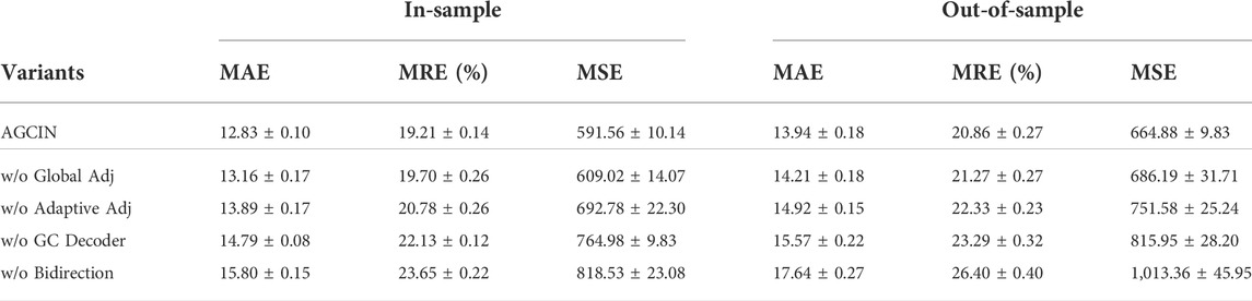
TABLE 3. Ablation study of the variants of proposed AGCIN by removing different designed modules.

5.5 Robustness analysis

To study the robustness of the proposed framework, we conducted an assessment of performance degradation across varied data missingness ratios. Specifically, we trained a model for AGCIN by randomly masking out a certain proportion of input data for each batch during training, then we ran the model on the test set. The testing results across varied data missingness ratios in three datasets are provided in Figure 3. It is observed that the performance degradation of AGCIN is negligible while the ratio is below 0.3. The imputation accuracy would be greatly affected when over 70% of the data are missing during training.

FIGURE 3

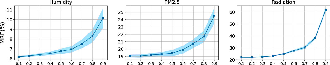
FIGURE 3. Imputation performance across varied data missingness ratios on the three datasets.

Also, we carried out an assessment of competitive baselines under different amounts of data missing. A comparison of their performance with the proposed AGCIN is presented in Figure 4. With randomly missing ratios from 30% to 70%, AGCIN consistently performs the best in regards to imputation accuracy measured in MSE, and the performance degradation is slower than that of other methods as the missing ratio increases. GAIN fails to achieve good imputation accuracy, especially when the missing ratio reaches 50%. As over 60% of the data are masked out from training, the performance of AGCIN drops, especially for the radiation data imputation. It is worth to be noticed that, AGCIN, as well as many of the baseline methods, follows the autoregressive paradigm, which suffers from error accumulation over long time horizons.

FIGURE 4

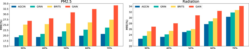
FIGURE 4. A comparison of baselines and AGCIN across varied data missingness ratios on PM2.5 and radiation datasets.

5.6 Visualization

As the final experiment, we provide a qualitative assessment of the learned graph. Figure 5 presents the changing patterns of a learned adjacency matrix defined in Eq. 5 in the training epochs 0, 10, 30, and 60. It is observed that during the training of AGCIN, the adjacency matrix is updated in each epoch and the graph topology constructed becomes more and more clear.

FIGURE 5

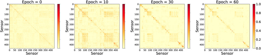
FIGURE 5. The change of adaptive adjacency matrix learned during model training.

To further examine the quality of the learned graph, we selected a group of sensors (sensors 413, 414, and 416) in the air quality sensor network with high weights ($>$0.5) in the learned adjacency matrix and plot their PM2.5 recordings and the imputed values by the proposed AGCIN. According to Figure 6, the ground truth sequences of the three sensors present similar changing patterns of air pollutants and AGCIN well captures the trends, which validates the proposed framework’s ability in modeling spatio-temporal dependencies in the imputation task. This qualitative observation verifies the effectiveness of the adaptive graph learning strategy in our approach.

FIGURE 6

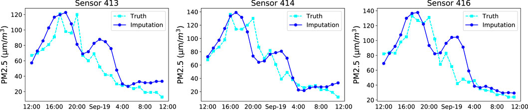
FIGURE 6. Plot of imputations of three air quality sensors with high weights in the learned adjacency matrix.

6 Conclusion

This paper proposes a graph structure learning-based framework that adaptively models spatio-temporal dependencies for environmental sensor data recovery. By leveraging the Canberra distance to measure feature similarity, we design an initial graph generator to obtain a good estimate of the graph structure. Also, an adaptive graph learning module is incorporated to learn latent node representations in a sensor network, and the learned node embeddings are integrated to construct the graph topology with the bidirectional GRU to recover the missing values via a two-stage imputation. The experiments on three real-world datasets demonstrate the effectiveness of AGCIN for enhancing the imputation accuracy in environmental sensor networks.

Data availability statement

One public dataset and two originally aggregated datasets were used in this study. The datasets and code are available at: https://github.com/Fanglanc/AGCIN.

Author contributions

FC and DW conceived of the presented idea. FC and SL carried out the experiments. JH helped the design of figures and tables. FC wrote the manuscript with support from DW, YF and C-TL. All authors discussed the results and improved the representation and language of the final manuscript.

Funding

This research was partially supported by Virginia Tech’s Open Access Subvention Fund, and the National Science Foundation (NSF) via the grant numbers: IIS-2045567, IIS-2006889, IIS-2040950, IIS-1755946.

Conflict of interest

The authors declare that the research was conducted in the absence of any commercial or financial relationships that could be construed as a potential conflict of interest.

Publisher’s note

All claims expressed in this article are solely those of the authors and do not necessarily represent those of their affiliated organizations, or those of the publisher, the editors and the reviewers. Any product that may be evaluated in this article, or claim that may be made by its manufacturer, is not guaranteed or endorsed by the publisher.

References

Androutsos, D., Plataniotiss, K., and Venetsanopoulos, A. N. (1998). “Distance measures for color image retrieval,” in Proceedings 1998 International Conference on Image Processing. ICIP98 (Cat. No. 98CB36269), Chicago, IL, USA, October 4-7, 1998. (IEEE), 770–774.

Google Scholar

Atwood, J., and Towsley, D. (2016). Diffusion-convolutional neural networks. Adv. neural Inf. Process. Syst. 29, 2001–2009. doi:10.5555/3157096.3157320

CrossRef Full Text | Google Scholar

Bai, S., Kolter, J. Z., and Koltun, V. (2018). An empirical evaluation of generic convolutional and recurrent networks for sequence modeling. arXiv preprint arXiv:1803.01271. Available at: https://arxiv.org/abs/1803.01271 (Accessed 4 Mar 2018).

Google Scholar

Beretta, L., and Santaniello, A. (2016). Nearest neighbor imputation algorithms: A critical evaluation. BMC Med. Inf. Decis. Mak. 16, 74–208. doi:10.1186/s12911-016-0318-z

PubMed Abstract | CrossRef Full Text | Google Scholar

Burda, Y., Grosse, R., and Salakhutdinov, R. (2015). Importance weighted autoencoders. arXiv preprint arXiv:1509.00519. Available at: https://arxiv.org/abs/1509.00519 (Accessed 1 Sep 2015).

Google Scholar

Cai, D., He, X., Han, J., and Huang, T. S. (2010). Graph regularized nonnegative matrix factorization for data representation. IEEE Trans. Pattern Anal. Mach. Intell. 33, 1548–1560. doi:10.1109/TPAMI.2010.231

PubMed Abstract | CrossRef Full Text | Google Scholar

Cai, L., Janowicz, K., Mai, G., Yan, B., and Zhu, R. (2020). Traffic transformer: Capturing the continuity and periodicity of time series for traffic forecasting. Trans. GIS 24, 736–755. doi:10.1111/tgis.12644

CrossRef Full Text | Google Scholar

Candès, E. J., and Recht, B. (2009). Exact matrix completion via convex optimization. Found. Comut. Math. 9, 717–772. doi:10.1007/s10208-009-9045-5

CrossRef Full Text | Google Scholar

Cao, W., Wang, D., Li, J., Zhou, H., Li, L., and Li, Y. (2018). Brits: Bidirectional recurrent imputation for time series. Advances in neural information processing systems. Available at: https://arxiv.org/abs/1805.10572 (Accessed May 27, 2018).

Google Scholar

Che, Z., Purushotham, S., Cho, K., Sontag, D., and Liu, Y. (2018). Recurrent neural networks for multivariate time series with missing values. Sci. Rep. 8, 6085. doi:10.1038/s41598-018-24271-9

PubMed Abstract | CrossRef Full Text | Google Scholar

Choi, C., Jung, H., and Cho, J. (2021). An ensemble method for missing data of environmental sensor considering univariate and multivariate characteristics. Sensors 21, 7595. doi:10.3390/s21227595

PubMed Abstract | CrossRef Full Text | Google Scholar

Chung, J., Gulcehre, C., Cho, K., and Bengio, Y. (2014). Empirical evaluation of gated recurrent neural networks on sequence modeling. arXiv preprint arXiv:1412.3555. Available at: https://arxiv.org/abs/1412.3555 (Accessed Dec 11, 2014).

Google Scholar

Cichocki, A., and Phan, A.-H. (2009). Fast local algorithms for large scale nonnegative matrix and tensor factorizations. IEICE Trans. Fundam. 92, 708–721. doi:10.1587/transfun.e92.a.708

CrossRef Full Text | Google Scholar

Cini, A., Marisca, I., and Alippi, C. (2021). Filling the g_ap_s: Multivariate time series imputation by graph neural networks. arXiv preprint arXiv:2108.00298. Available at: https://arxiv.org/abs/2108.00298 (Accessed Jul 31, 2021).

Google Scholar

Defferrard, M., Bresson, X., and Vandergheynst, P. (2016). Convolutional neural networks on graphs with fast localized spectral filtering. Adv. neural Inf. Process. Syst. 29, 3844–3852. doi:10.5555/3157382.3157527

CrossRef Full Text | Google Scholar

Di Nisio, A., Adamo, F., Acciani, G., and Attivissimo, F. (2020). Fast detection of olive trees affected by xylella fastidiosa from uavs using multispectral imaging. Sensors 20, 4915. doi:10.3390/s20174915

PubMed Abstract | CrossRef Full Text | Google Scholar

Ding, Y., Street, W. N., Tong, L., and Wang, S. (2019). “An ensemble method for data imputation,” in 2019 IEEE International Conference on Healthcare Informatics (ICHI), Xi'an, China, June 10-13, 2019. (IEEE), 1–3.

CrossRef Full Text | Google Scholar

Domínguez-Brito, A. C., Cabrera-Gámez, J., Viera-Pérez, M., Rodríguez-Barrera, E., and Hernández-Calvento, L. (2020). A diy low-cost wireless wind data acquisition system used to study an arid coastal foredune. Sensors 20, 1064. doi:10.3390/s20041064

CrossRef Full Text | Google Scholar

Durbin, J., and Koopman, S. J. (2012). Time series analysis by state space methods. Oxford, United Kingdom: OUP Oxford. 38.

Google Scholar

Ghahramani, Z., and Jordan, M. (1993). Supervised learning from incomplete data via an em approach. Adv. neural Inf. Process. Syst. 6, 120–127. doi:10.5555/2987189.2987205

CrossRef Full Text | Google Scholar

Goodfellow, I., Bengio, Y., and Courville, A. (2016). Deep learning. Massachusetts, United States: MIT press.

Google Scholar

Goodfellow, I., Pouget-Abadie, J., Mirza, M., Xu, B., Warde-Farley, D., Ozair, S., et al. (2014). Generative adversarial nets. Adv. neural Inf. Process. Syst. 27, 2672–2680. doi:10.5555/2969033.2969125

CrossRef Full Text | Google Scholar

Gruenwald, L., Chok, H., and Aboukhamis, M. (2007). “Using data mining to estimate missing sensor data,” in Seventh IEEE international conference on data mining workshops (ICDMW 2007) (IEEE), 207–212.

CrossRef Full Text | Google Scholar

Ibrahim, D. S., Mahdi, A. F., and Yas, Q. M. (2021). Challenges and issues for wireless sensor networks: A survey. J. Glob. Sci. Res. 6, 1079–1097.

Google Scholar

Kipf, T., Fetaya, E., Wang, K.-C., Welling, M., and Zemel, R. (2018). “Neural relational inference for interacting systems,” in International Conference on Machine Learning (PMLR), Stockholm, Sweden, July 10-15, 2018, 2688–2697.

Google Scholar

Kuppannagari, S. R., Fu, Y., Chueng, C. M., and Prasanna, V. K. (2021). “Spatio-temporal missing data imputation for smart power grids,” in Proceedings of the Twelfth ACM International Conference on Future Energy Systems, Virtual Event Italy, June 28-July 2, 2021, 458–465.

CrossRef Full Text | Google Scholar

Lanzolla, A., and Spadavecchia, M. (2021). Wireless sensor networks for environmental monitoring. Sensors (Basel) 21 (4), 1172. doi:10.3390/s21041172

PubMed Abstract | CrossRef Full Text | Google Scholar

LeCun, Y., Bengio, Y., and Hinton, G. (2015). Deep learning. nature 521, 436–444. doi:10.1038/nature14539

PubMed Abstract | CrossRef Full Text | Google Scholar

Li, Y., Yu, R., Shahabi, C., and Liu, Y. (2017). Diffusion convolutional recurrent neural network: Data-driven traffic forecasting. arXiv preprint arXiv:1707.01926. Available at: https://arxiv.org/abs/1707.01926 (Accessed Jul 6, 2017).

Google Scholar

Lipton, Z. C., Kale, D., and Wetzel, R. (2016). “Directly modeling missing data in sequences with rnns: Improved classification of clinical time series,” in Machine learning for healthcare conference (PMLR), Los Angeles, CA, USA, August 19-20, 2016, 253–270.

Google Scholar

Liu, Y., Yu, R., Zheng, S., Zhan, E., and Yue, Y. (2019). Naomi: Non-autoregressive multiresolution sequence imputation. Adv. neural Inf. Process. Syst. 32, 11236–11246.

Google Scholar

Luo, L., Qin, H., Song, X., Wang, M., Qiu, H., and Zhou, Z. (2020). Wireless sensor networks for noise measurement and acoustic event recognitions in urban environments. Sensors 20, 2093. doi:10.3390/s20072093

PubMed Abstract | CrossRef Full Text | Google Scholar

Luo, Y., Cai, X., Zhang, Y., Xu, J., and xiaojie, Y. (2018). Multivariate time series imputation with generative adversarial networks. Adv. neural Inf. Process. Syst. 31, 1603–1614. doi:10.5555/3326943.3327090

CrossRef Full Text | Google Scholar

Luo, Y., Zhang, Y., Cai, X., and Yuan, X. (2019). “E2gan: End-to-end generative adversarial network for multivariate time series imputation,” in Proceedings of the 28th international joint conference on artificial intelligence, Macao, China, August 10-16, 2019 (Palo Alto, CA, USA: AAAI Press), 3094–3100.

Google Scholar

Lütkepohl, H. (2013). “Vector autoregressive models,” in Handbook of research methods and applications in empirical macroeconomics (Cheltenham, United Kingdom: Edward Elgar Publishing), 139–164.

Google Scholar

Ma, C., Gong, W., Hernández-Lobato, J. M., Koenigstein, N., Nowozin, S., and Zhang, C. (2018a). “Partial vae for hybrid recommender system,” in NIPS Workshop on Bayesian Deep Learning, Montréal, Canada, December 7, 2018.

Google Scholar

Ma, C., Tschiatschek, S., Palla, K., Hernández-Lobato, J. M., Nowozin, S., and Zhang, C. (2018b). Eddi: Efficient dynamic discovery of high-value information with partial vae. arXiv preprint arXiv:1809.11142. Available at: https://arxiv.org/abs/1809.11142 (Accessed Sep 28, 2018).

Google Scholar

Mattei, P.-A., and Frellsen, J. (2018). Leveraging the exact likelihood of deep latent variable models. Adv. Neural Inf. Process. Syst. 31, 3859–3870. doi:10.5555/3327144.3327301

CrossRef Full Text | Google Scholar

Mattei, P.-A., and Frellsen, J. (2019). “Miwae: Deep generative modelling and imputation of incomplete data sets,” in International conference on machine learning (PMLR), Long Beach, CA, USA, June 10-15, 2019, 4413–4423.

Google Scholar

Mei, J., De Castro, Y., Goude, Y., and Hébrail, G. (2017). “Nonnegative matrix factorization for time series recovery from a few temporal aggregates,” in International Conference on Machine Learning (PMLR), Sydney, Australia, August 6-11, 2017, 2382–2390.

Google Scholar

Miao, X., Wu, Y., Wang, J., Gao, Y., Mao, X., and Yin, J. (2021). Generative semi-supervised learning for multivariate time series imputation. Proc. AAAI Conf. Artif. Intell. 35, 8983–8991. doi:10.1609/aaai.v35i10.17086

CrossRef Full Text | Google Scholar

Nazabal, A., Olmos, P. M., Ghahramani, Z., and Valera, I. (2020). Handling incomplete heterogeneous data using vaes. Pattern Recognit. 107, 107501. doi:10.1016/j.patcog.2020.107501

CrossRef Full Text | Google Scholar

Nelwamondo, F. V., Mohamed, S., and Marwala, T. (2007). Missing data: A comparison of neural network and expectation maximization techniques. Curr. Sci. 93, 1514–1521.

Google Scholar

Paassen, B., Grattarola, D., Zambon, D., Alippi, C., and Hammer, B. E. (2020). “Graph edit networks,” in International Conference on Learning Representations, Addis Ababa, Ethiopia, April 26-30, 2020.

Google Scholar

Qin, H., Zhan, X., Li, Y., Yang, X., and Zheng, Y. (2021). “Network-wide traffic states imputation using self-interested coalitional learning,” in Proceedings of the 27th ACM SIGKDD Conference on Knowledge Discovery & Data Mining, Virtual Event Singapore, August 14-18, 2021, 1370–1378.

CrossRef Full Text | Google Scholar

Rao, N., Yu, H.-F., Ravikumar, P. K., and Dhillon, I. S. (2015). Collaborative filtering with graph information: Consistency and scalable methods. Adv. neural Inf. Process. Syst. 28, 2107–2115. doi:10.5555/2969442.2969475

CrossRef Full Text | Google Scholar

Rezende, D. J., Mohamed, S., and Wierstra, D. (2014). “Stochastic backpropagation and approximate inference in deep generative models,” in International conference on machine learning (PMLR), 1278–1286.

Google Scholar

Richardson, T. W., Wu, W., Lin, L., Xu, B., and Bernal, E. A. (2020). “Mcflow: Monte Carlo flow models for data imputation,” in Proceedings of the IEEE/CVF Conference on Computer Vision and Pattern Recognition, 14205–14214.

CrossRef Full Text | Google Scholar

Rubin, D. B. (1976). Inference and missing data. Biometrika 63, 581–592. doi:10.1093/biomet/63.3.581

CrossRef Full Text | Google Scholar

Schmidhuber, J. (2015). Deep learning in neural networks: An overview. Neural Netw. 61, 85–117. doi:10.1016/j.neunet.2014.09.003

PubMed Abstract | CrossRef Full Text | Google Scholar

Seo, Y., Defferrard, M., Vandergheynst, P., and Bresson, X. (2018). “Structured sequence modeling with graph convolutional recurrent networks,” in International conference on neural information processing, Siem Reap, Cambodia, December 13-16, 2018 (Springer), 362–373.

CrossRef Full Text | Google Scholar

Shang, C., Chen, J., and Bi, J. (2021). Discrete graph structure learning for forecasting multiple time series. arXiv preprint arXiv:2101.06861. Available at: https://arxiv.org/abs/2101.06861 (Accessed Jan 18, 2021).

Google Scholar

Shuman, D. I., Narang, S. K., Frossard, P., Ortega, A., and Vandergheynst, P. (2013). The emerging field of signal processing on graphs: Extending high-dimensional data analysis to networks and other irregular domains. IEEE Signal Process. Mag. 30, 83–98. doi:10.1109/msp.2012.2235192

CrossRef Full Text | Google Scholar

Spinelli, I., Scardapane, S., and Uncini, A. (2020). Missing data imputation with adversarially-trained graph convolutional networks. Neural Netw. 129, 249–260. doi:10.1016/j.neunet.2020.06.005

PubMed Abstract | CrossRef Full Text | Google Scholar

Stekhoven, D. J., and Bühlmann, P. (2012). Missforest—Non-parametric missing value imputation for mixed-type data. Bioinformatics 28, 112–118. doi:10.1093/bioinformatics/btr597

PubMed Abstract | CrossRef Full Text | Google Scholar

Troyanskaya, O., Cantor, M., Sherlock, G., Brown, P., Hastie, T., Tibshirani, R., et al. (2001). Missing value estimation methods for dna microarrays. Bioinformatics 17, 520–525. doi:10.1093/bioinformatics/17.6.520

PubMed Abstract | CrossRef Full Text | Google Scholar

Vaswani, A., Shazeer, N., Parmar, N., Uszkoreit, J., Jones, L., Gomez, A. N., et al. (2017). Attention is all you need. Adv. neural Inf. Process. Syst. 30, 6000–6010. doi:10.5555/3295222.3295349

CrossRef Full Text | Google Scholar

Walter, Y., Kihoro, J., Athiany, K., and Kibunja, H. (2013). Imputation of incomplete non-stationary seasonal time series data. Math. Theory Model 3, 142–154.

Google Scholar

White, I. R., Royston, P., and Wood, A. M. (2011). Multiple imputation using chained equations: Issues and guidance for practice. Stat. Med. 30, 377–399. doi:10.1002/sim.4067

PubMed Abstract | CrossRef Full Text | Google Scholar

Wu, Z., Pan, S., Long, G., Jiang, J., Chang, X., and Zhang, C. (2020). “Connecting the dots: Multivariate time series forecasting with graph neural networks,” in Proceedings of the 26th ACM SIGKDD international conference on knowledge discovery & data mining, 753–763.

CrossRef Full Text | Google Scholar

Wu, Z., Pan, S., Long, G., Jiang, J., and Zhang, C. (2019). Graph wavenet for deep spatial-temporal graph modeling. arXiv preprint arXiv:1906.00121. Available at: https://arxiv.org/abs/1906.00121 (Accessed May 31, 2019).

CrossRef Full Text | Google Scholar

Yi, X., Zheng, Y., Zhang, J., and Li, T. (2016). “St-mvl: Filling missing values in geo-sensory time series data,” in Proceedings of the 25th International Joint Conference on Artificial Intelligence.

Google Scholar

Yoon, J., Jordon, J., and Schaar, M. (2018a). “Gain: Missing data imputation using generative adversarial nets,” in International conference on machine learning (PMLR), 5689–5698.

Google Scholar

Yoon, J., Zame, W. R., and van der Schaar, M. (2018b). Estimating missing data in temporal data streams using multi-directional recurrent neural networks. IEEE Trans. Biomed. Eng. 66, 1477–1490. doi:10.1109/tbme.2018.2874712

PubMed Abstract | CrossRef Full Text | Google Scholar

You, J., Ma, X., Ding, Y., Kochenderfer, M. J., and Leskovec, J. (2020). Handling missing data with graph representation learning. Adv. Neural Inf. Process. Syst. 33, 19075–19087. doi:10.5555/3495724.3497325

CrossRef Full Text | Google Scholar

Yu, B., Yin, H., and Zhu, Z. (2017). Spatio-temporal graph convolutional networks: A deep learning framework for traffic forecasting. arXiv preprint arXiv:1709.04875. Available at: https://arxiv.org/abs/1709.04875 (Accessed Sep 14, 2017).

Google Scholar

Yu, H.-F., Rao, N., and Dhillon, I. S. (2016). Temporal regularized matrix factorization for high-dimensional time series prediction. Adv. neural Inf. Process. Syst. 29, 847–855. doi:10.5555/3157096.3157191

CrossRef Full Text | Google Scholar

Zambon, D., Grattarola, D., Livi, L., and Alippi, C. (2019). “Autoregressive models for sequences of graphs,” in 2019 International Joint Conference on Neural Networks (IJCNN), Budapest, Hungary, July 14-19, 2019. (IEEE), 1–8.

CrossRef Full Text | Google Scholar

Zhang, J., Shi, X., Xie, J., Ma, H., King, I., and Yeung, D.-Y. (2018). Gaan: Gated attention networks for learning on large and spatiotemporal graphs. arXiv preprint arXiv:1803.07294. Available at: https://arxiv.org/abs/1803.07294 (Accessed Mar 20, 2018).

Google Scholar