Comparative study on numerical simulation based on CALPUFF and wind tunnel simulation of hazardous chemical leakage accidents

CALPUFF, as a Lagrangian puff modeling system, is mostly used in the field of atmospheric environment research and risk assessment. CALPUFF performs well for short-term and short-range release scenarios over complex terrain, as well as long-term and long-range transportation. Therefore, this article uses the CALPUFF model to simulate a toxic gas leakage accident in a hazardous chemical plant in an urban area, focusing on the influence of local buildings. Wind tunnel experiments are performed in accordance with the CALPUFF experiments to assess the model’s accuracy in cases of chemical leakage accidents. The results of the wind tunnel experiment are superimposed on the map of CALPUFF calculation, and the quantitative analysis is also performed. The comparative results show that the simulation results of the CALPUFF are mainly affected by factors such as wind direction, wind speed, and the complexity of the surface environment. With less influence of buildings, such as the south and north wind, the CALPUFF simulation is consistent with the wind tunnel experiment, having a correlation coefficient of over 0.7 in most cases, while under the east wind, the consistency is significantly lower due to the influence of buildings. In addition, it is found that the wind tunnel experiment is more accurate in the near field of the pollution source, while CALPUFF is more suitable for simulating the overall trend of gas dispersion. The comparison and evaluation of the capabilities of different methods on gas dispersion simulation are helpful in guiding the emergency response during hazardous chemical leakage accidents.

1 Introduction

A gas dispersion model studies the complex hydrodynamic processes of pollutants, such as diffusion, transportation, transformation, and deposition in the atmosphere. A gas dispersion model usually can be described as a set of computable mathematical formulas through reasonable physical and chemical assumptions. Generally, gas dispersion models can be divided into the box model, Gaussian model, Lagrangian model, Euler model, and computational fluid dynamics model (Holmes et al., 2006), according to the fundamental principles. The last four types of models are most commonly used.

The Gaussian model includes a plume model and a puff model, and the model systems of this type commonly used are ADMS (Carruthers et al., 1994), AERMOD (Cimorelli et al., 2004), and ALOHA (NOAA and EPA, 2007). The plume model considers gas emitted continuously, and the pollutant concentration distribution is compliant with the rule of Gaussian distribution, while the puff model considers the continuously emitted plume as a series of discrete pollutant masses, namely, the air mass. The emission of air mass is instantaneous, whose movement is affected by the wind direction and wind speed. The concentration distribution of the air masses conforms to Gaussian distribution, and the concentration of the pollutant at each receptor point is the linear superposition of the concentration value of each air mass here (Yuan et al., 2013). The Lagrangian model includes a particle model and a puff model, whose common model systems include HYSPLIT (Stein et al., 2015) and NAME (Jones et al., 2007). The particle model is a dispersion model based on the statistical theory of turbulence, which calculates the temporal and spatial probability distribution of particles by recording the movement track of the labeled particles so as to estimate the variation of the pollutant concentration. In the puff model, it is assumed that the concentration distribution of the puff satisfies Gaussian distribution in both horizontal and vertical directions (Yu and Cao, 2020). The Euler model, similar to the computational fluid dynamics model, is a kind of grid model that uses numerical methods to discretely solve the convection–dispersion equation for the concentration derived from the law of conservation of mass and Fick’s Law (Stockie, 2011).

The gas dispersion model can be used not only in regional ecological monitoring and environmental pollution control but also in emergency response management. The research and applications of the gas dispersion model in the emergency field mainly concentrate on the nuclear accident (Liu et al., 2017; Li et al., 2018; Ulimoen et al., 2022), chemical industrial park (Huang et al., 2019; Cheng et al., 2021), gas pipeline (Mishra et al., 2015 CFD; Yan et al., 2016), and road transportation (Fallah-Shorshani et al., 2015; Kota et al., 2013). Compared with the environmental assessment cases, the emergency simulation often requires a near-field, finer spatial-temporal computational grid and further analysis and adjustment of the model parameters (Rzeszutek, 2019).

The validation study on the gas dispersion model is helpful in evaluating its applicability and prediction accuracy in different meteorology, terrain, and pollution source conditions so as to better guide model selection and parameter setting of different simulation scenarios. At present, many verification studies compare the field observation data on sampling points with the model simulation data. For example, Masoud Fallah–Shorshani used the composite model chain combining traffic, emission, and dispersion models to simulate the NO₂ pollution concentration of urban blocks and compared it with the observation data on measurement stations (Fallah-Shorshani et al., 2017). Piotr Holnicki used the CALPUFF model to simulate the annual average concentration of air pollutants in major cities in Warsaw and the hourly average concentration of air pollutants on a certain day and compared with the data on five observation stations, finding that the CALPUFF model has a higher accuracy of simulation on a long-time scale (Holnicki et al., 2016). In order to evaluate the simulation results of AERMOD, CALPUFF, ISC2, and RATCHET models, AS Rood used the dataset of the 1991 experiment in the Rocky Mountains for model verification, in which 140 sampling sites were distributed within 16 km from the pollution source, including 12 independent experiments (Rood, 2014). Although the field experiment can better represent the reality and has high reliability, its operation process is complex and time-consuming, and the number of sampling points is limited. In addition, the location and the pollutant type of field observations are limited. It is impossible to carry out experiments of toxic gases or in crowded areas.

Therefore, some studies use wind tunnel experimental data to verify the gas dispersion models. For example, Dong et al. (2021) carried out wind tunnel experiments in six directions of the Sanmen nuclear power plant area and compared the results of the wind field and concentration field qualitatively and quantitatively with the simulation results of CALMET-RIMPUFF and SWIFT-RIMPUFF models, respectively. Toscano et al. (2021) used the wind tunnel experiment and CFD numerical simulation to evaluate the emission impact of cruise ships berthing at the port of Naples and verified the accuracy of the CALPUFF model. Yassin et al. (2021) conducted the numerical simulation of pollution gas emissions from urban roof chimneys and verified with wind tunnel experiment results both qualitatively and quantitatively. Jiang et al. (2021) carried out wind tunnel experiments in eight directions on leakage and diffusion accidents of high sulfur gas in mountainous terrain and drew the risk distribution map. Comparing with the CFD simulation results, they found that the numerical simulation accuracy was not enough and proposed an improved numerical simulation equation. In wind tunnel experiments, the properties of the gas airflow, such as pressure, velocity, temperature, and density, can be adjusted easily and accurately. In addition, an indoor experiment is safer and more flexible. So, experiments under different conditions can be carried out at once.

The technical guidelines for the environmental impact assessment-Atmospheric Environment (HJ 2.2-2018) issued by the Ministry of Ecology and Environment of China have recommended gas dispersion models which have been extensively utilized in environmental assessment and the evaluation of atmospheric environmental quality. Among them, the CALPUFF model is suitable for long-scale experimental areas (more than 50 km), comprehensively considering complex terrain, meteorological parameters, and other aspects and has higher accuracy (Li et al., 2020; Ridzuan et al., 2020). Compared with other gas dispersion models, CALPUFF computes more rapidly than the CFD model and supports finer spatial and temporal resolutions than other Gaussian models like AERMOD. Based on the aforementioned factors, the CALPUFF model is selected for emergency simulation in this study.

However, there are few studies that validate the accuracy of CALPUFF in small-scale emergency scenarios, which could offer important reference for many industries like oil and gas field. In this paper, a comparative study between the CALPUFF model and wind tunnel experiment on toxic gas leakage accidents in the near-field area is conducted. An ethylene gas leakage accident case in a national hazardous chemical emergency rescue (training) center is simulated both from the CALPUFF simulation and wind tunnel experiment, followed by qualitative and quantitative comparisons. Finally, the effect of the CALPUFF model on near-field diffusion simulation in urban areas with dense buildings is validated.

2 Methods

2.1 CALPUFF model

The CALPUFF model is a new generation of the unsteady gas phase and air quality modeling system developed by Sigma Corporation of America, as one of the Lagrange–Gaussian puff models (Scire et al., 2011). It divides the pollutants into several puffs according to a certain volume, where the Lagrangian method is used to calculate the trajectory of the puffs, and the Gaussian method is used to calculate the distribution of pollutants inside a puff. Finally, each puff is superimposed to obtain the total concentration field. The model adopts the meteorological data of the hourly wind field, fully considers the influence of a complex terrain on the dry and wet deposition of pollutants, and simulates the diffusion pattern of pollutants in areas of different scales well. The CALPUFF model is mainly composed of four parts: the geographic and meteorological data preprocessors, meteorological model CALMET, dispersion model CALPUFF, and postprocessor CALPOST, as shown in Figure 1.

FIGURE 1

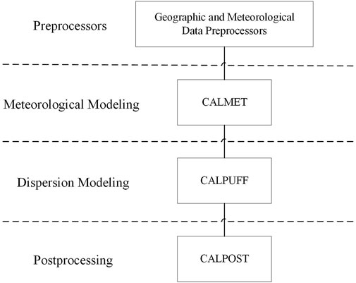
FIGURE 1. Main system modules of the CALPUFF model.

2.1.1 Diagnostic wind model

CALMET includes a diagnostic wind model and a micrometeorological model. The workflow of the diagnostic wind model is shown in Figure 2.

FIGURE 2

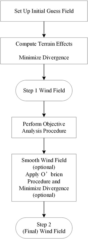
FIGURE 2. Main process of the CALMET module.

The CALMET diagnostic wind model uses two steps to estimate the wind field. It should be noted that the initial gas field can be a three-dimensional wind field or a constant wind field composed of regional average. The regional average wind field can be obtained by means of the vertical average and temporal interpolation of meteorological data from high-altitude observations or can be directly specified by users. If the regional average wind field is calculated, a user needs to specify not only the atmospheric layer for which the average wind field is to be calculated but also the high-altitude sounding stations for calculation. Alternatively, all station data are interpolated inversely to the square of the distance to produce an initial guess wind field with spatial variation. The first step is to calculate the step 1 wind field from the initial gas field, including adjustments for kinematic terrain effects, slope flows, blocking effect and a three-dimensional divergence minimization procedure, and other algorithms. The second step includes an objective analysis that introduces the observation data into the step 1 wind field to generate the final wind field, including interpolation, smoothing, O’Brien adjustment of vertical wind speed, divergence minimization, and other algorithms. We can also use grids to predict the wind field in CALMET, which better reflects some aspects of the regional flow, sea breeze circulation, and slope/valley circulation.

2.1.2 Lagrange–Gaussian puff model

CALPUFF is a puff model that simulates multilayer and multipollutant-type diffusion in unsteady conditions. It can simulate the migration, transformation, and dispersion of pollutants in meteorological conditions that vary temporarily and spatially. The main processes are as follows: retrieving and processing time-averaged data from meteorological and source information files; releasing, transporting, and removing puffs from computational grids; assessing the effects of diffusion, chemical conversion, dry and wet deposition, and subgrid-scale complex topography; and sampling puffs to obtain concentrations and deposition fluxes at the gridded and discrete receptors. Among them, the algorithms dealing with near-source influences include building downwash, transitional plume lifting, partial plume penetration, and subgrid terrain interaction. The algorithms dealing with long distance transmission influences include dry and wet deposition, chemical transformation, vertical wind shear, overwater transport, and coastal interaction effects.

Generally, the puff model evaluates the concentration contribution of a puff to a receptor point through the snapshot method. For example, if the time step is 1 h and the sampling step is 1 min, then the contribution of a puff to the receptor point’s 1-h average concentration will be the average of 60 snapshots per minute. The disadvantage of this method is that when the distance between puffs is too large and overlapping is not enough, the simulation results may be inaccurate, that is, the concentration of receptor points located in the gap between puffs at the sampling time will be lower than the real value, while the concentration of those in the center of puffs will be higher. There are two sampling functions in CALPUFF to solve this problem: the first is a radially symmetric Gaussian puff, and the second is a non-circular puff stretched in the direction of the wind, when released, called slug, does not need to release the puff frequently. For most CALPUFF applications, the modeling of emissions as puffs is recommended as it produces similar model results but with significantly shorter run times than the slug approach. However, the slug approach is preferred for causality effects along small spatial and temporal scales, such as an accidental release scenario, and where the transport from the source to the receptor is very short. Therefore, this study chooses the slug function.

The basic equations of the puff sampling function are as follows:

$\mathit{c}\left(\mathit{x},\mathit{y},\mathit{z}\right)=\frac{\mathit{Q}}{\mathbf{2}\mathit{\pi }{\mathit{\sigma }}_{\mathit{x}}{\mathit{\sigma }}_{\mathit{y}}}\mathit{g}\bullet \mathit{exp}\left(-\frac{{\mathit{d}}_{\mathit{a}}^{\mathbf{2}}}{\mathbf{2}{\mathit{\sigma }}_{\mathit{x}}^{\mathbf{2}}}\right)\mathit{exp}\left(-\frac{{\mathit{d}}_{\mathit{b}}^{\mathbf{2}}}{\mathbf{2}{\mathit{\sigma }}_{\mathit{y}}^{\mathbf{2}}}\right),(1)$

$\mathit{g}=\frac{\mathbf{2}}{\sqrt{\mathbf{2}\mathit{\pi }}{\mathit{\sigma }}_{\mathit{z}}}\underset{\mathit{n}=-\mathit{\infty }}{{\displaystyle \sum }^{\infty }}\mathit{exp}\left(-\frac{{\left(\mathit{H}+\mathbf{2}\mathit{n}\mathit{h}\right)}^{\mathbf{2}}}{\mathbf{2}{\mathit{\sigma }}_{\mathit{z}}^{\mathbf{2}}}\right),(2)$

where c(x,y,z) is the ground-level concentration of the pollutant at a specific receptor; Q is the pollutant mass in the puff; x, y, and z still represent the along-wind, cross-wind, and vertical directions, respectively; σ_x, σ_y, and σ_z are the standard deviations of the Gaussian distribution in the three directions, respectively; and d_a and d_b are the distances from the puff center to the receptor in the along-wind and cross-wind directions, respectively. g is the vertical term of the Gaussian equation, H is the effective height above the ground of the puff center, and h is the mixed-layer height. The summation in the vertical term, g, accounts for multiple reflections of the mixing lid and the ground. It reduces to the uniformly mixed limit of 1/h for σ_z > 1.6h. In general, puffs within the convective boundary layer meet this criterion within a few hours after release.

For a horizontally symmetric puff, with σ_x = σ_y, Eq. 1 reduces to

$\mathit{c}\left(\mathit{s}\right)=\frac{\mathit{Q}\left(s\right)}{\mathbf{2}\pi {\mathit{\sigma }}_{\mathit{y}}^{\mathbf{2}}\left(\mathit{s}\right)}\mathit{g}\left(\mathit{s}\right)\bullet \mathit{exp}\left(-\frac{{\mathit{R}}^{\mathbf{2}}\left(\mathit{s}\right)}{\mathbf{2}{\sigma }_{\mathit{y}}^{\mathbf{2}}\left(\mathit{s}\right)}\right),(3)$

where R is the distance from the center of the puff to the receptor and s is the distance traveled by the puff. An analytical solution to this integral can be obtained if s is the main variable. Generally, σ_y and g are computed at the mid-point of the trajectory segment because at mesoscale distances, the fractional change in the puff size during the sampling step is usually small, and the use of the mid-point values is adequate. This method for mesoscale distances, however, may not be appropriate in the near field, where the fractional puff growth rate can be rapid and plume height may vary. For this reason, the integrated sampling function has been implemented with receptor-specific values for σ_y and g and evaluated at the point of the closest approach of the puff to each receptor.

2.2 Building downwash

The building downwash effect is due to the air disturbance caused by buildings around the pollution source, resulting in the streamline sliding effect of the airflow emitted by the chimney after passing the building, which quickly diffuses to the ground, leading to a high local concentration. In the CALPUFF model, the parameterization of building downwash is suitable for use in the turbulent wake region and is based on the procedures used in the ISC3 model. ISC3 contains two building downwash algorithms:

(1) Huber–Snyder model (Huber and Synder, 1976; Huber, 1977). This model is applied when the source height H_s is greater than H_b+ 0.5L_b (H_b is the building height, and L_b is the lesser of the building height or the projected width). The first step is to compute the effective plume height, H_e, due to the momentum rise at a downwind distance of two building heights. If H_e exceeds H_b+1.5L_b, building downwash effects are assumed to be negligible. Otherwise, building-induced enhancement of the plume dispersion coefficients is evaluated. For stack heights, H_s, less than 1.2H_b, and both σ_y and σ_z are enhanced. Only σ_z is enhanced for stack heights above 1.2H_b (but below H_b+ 1.5 L_b).

For a squat building (that is, the projected building width exceeds its height, i.e., H_w ≥ H_b), the enhanced σ_y and σ_z can be calculated as follows:

${\mathit{\sigma }}_{\mathit{z}}^{\prime }=\mathbf{0.7}{\mathit{H}}_{\mathit{b}}+\mathbf{0.067}\left(\mathit{x}-\mathbf{3}{\mathit{H}}_{\mathit{b}}\right),(4)$

${\mathit{\sigma }}_{\mathit{y}}^{\prime }=\mathbf{0.35}{\mathit{H}}_{\mathit{w}}+\mathbf{0.067}\left(\mathit{x}-\mathbf{3}{\mathit{H}}_{\mathit{b}}\right)\mathrm{w}\mathrm{h}\mathrm{e}\mathrm{n}\mathrm{H}\mathrm{w}/\mathrm{H}\mathrm{b}<5,(5)$

${\mathit{\sigma }}_{\mathit{y}}^{\prime }=\mathbf{0.35}{\mathit{H}}_{\mathit{b}}+\mathbf{0.067}\left(\mathit{x}-\mathbf{3}{\mathit{H}}_{\mathit{b}}\right)\mathbf{o}\mathbf{r}{\mathit{\sigma }}_{\mathit{y}}^{\prime }=\mathbf{1.75}{\mathit{H}}_{\mathit{b}}+\mathbf{0.067}\left(\mathit{x}-\mathbf{3}{\mathit{H}}_{\mathit{b}}\right)\mathbf{w}\mathbf{h}\mathbf{e}\mathbf{n}\mathit{H}\mathit{w}/\mathit{H}\mathit{b}>\mathbf{5}.(6)$

For a tall building (that is, the building width exceeds its projected width, H_b ≥ H_w), the enhanced σ_y and σ_z can be calculated as follows:

${\mathit{\sigma }}_{\mathit{z}}^{\prime }=\mathbf{0.7}{\mathit{H}}_{\mathit{w}}+\mathbf{0.067}\left(\mathit{x}-\mathbf{3}{\mathit{H}}_{\mathit{w}}\right),(7)$

${\mathit{\sigma }}_{\mathit{y}}^{\prime }=\mathbf{0.35}{\mathit{H}}_{\mathit{w}}+\mathbf{0.067}\left(\mathit{x}-\mathbf{3}{\mathit{H}}_{\mathit{w}}\right).(8)$

(2) Schulman–Scire model (Schulman and Scire, 1980; Schulman and Hanna, 1986). This model applies a linear decay factor to the building-included enhancement of the dispersion coefficients and accounts for the effect of downwash on plume rise. It is used for stacks lower in height than H_b+ 0.5L_b. The main features of the algorithm are that the effects of building downwash on reducing the plume rise are incorporated, and the enhancement of σ_z is a gradual function of the effective plume height rather than a step function. The vertical dispersion coefficient is determined as follows:

${\mathit{\sigma }}_{\mathit{z}}^{″}=\mathit{A}{\mathit{\sigma }}_{\mathit{z}}^{\prime },(9)$

where σ_z' is determined from Eqs 4, 7, and

$\mathit{A}=\{\begin{array}{cc}\mathbf{1}& {\mathit{H}}_{\mathit{e}}\le {\mathit{H}}_{\mathit{b}}\\ \frac{{\mathit{H}}_{\mathit{b}}-{\mathit{H}}_{\mathit{e}}}{\mathbf{2}{\mathit{L}}_{\mathit{b}}}+\mathbf{1}& {\mathit{H}}_{\mathit{b}}<{\mathit{H}}_{\mathit{e}}{\le \mathit{H}}_{\mathit{b}}+\mathbf{2}{\mathit{L}}_{\mathit{b}}.\\ \mathbf{0}& {\mathit{H}}_{\mathit{b}}+\mathbf{2}{\mathit{L}}_{\mathit{b}}<{\mathit{H}}_{\mathit{e}}\end{array}(10)$

3 Experiments

3.1 CALPUFF configurations

This experimental area is located at a national hazardous chemical emergency rescue base, as shown in Figure 3. This base is a comprehensive training base integrating training, drill, appraisal, seminar, and competition regarding emergency firefighting. The base has 10 major training areas for fire training, smoke-heat simulation, oil and gas blowout, hazardous chemical leakage, building fire, earthquake prevention and disaster mitigation, three-dimensional desktop deduction, comprehensive physical exercise, water oil spill disposal, water rescue, and the large-scale oil pool fire experimental platform (600 m²). It can simulate the trainings of more than 130 emergency cases in 13 categories, such as petrochemical industrial leakage, earthquake, high-rise buildings, and water rescue. The base is built in a flat area, with a chemical factory on the westside and a farmland and villages on the other sides. The land covers good vegetation, and the trees are less than 10 m high.

FIGURE 3

FIGURE 3. Remote sensing image of the experimental area.

In this experiment, we assume that there is a chimney emitting stable ethylene (C₂H₄) in the middle of the research area. Gas tanks, office buildings, and other buildings around the chimney may block and divert gas dispersion. Configurations in CALPUFF are shown in Table 1.

TABLE 1

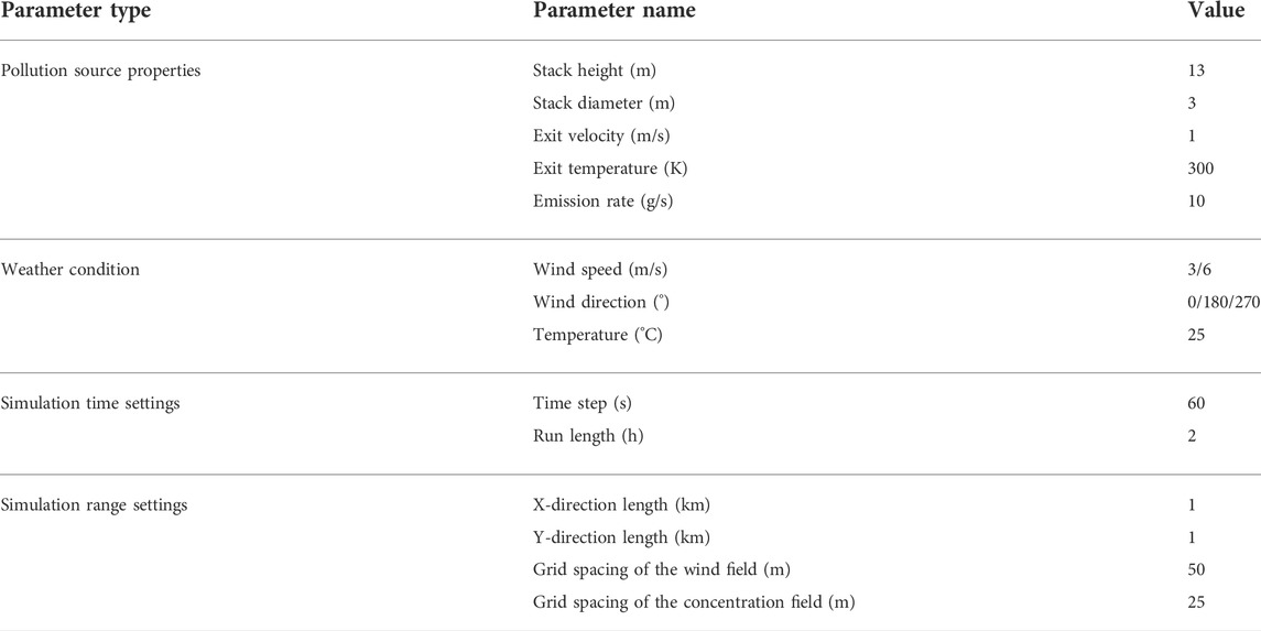
TABLE 1. Simulation parameters.

According to the remote sensing image of the base, the coordinates and height parameters of 14 major buildings, such as oil tanks, office buildings, and gas tanks, are collected and input into the building module of CALPUFF. The heights of the cylindrical tanks are about 10 m, and the heights of other buildings are about 2–8 m. Different discrete receptors are set under three wind directions, north, south, and east, and two wind speeds, 3 and 6 m/s (at the height of 10 m above the ground), as shown in Figure 4.

FIGURE 4

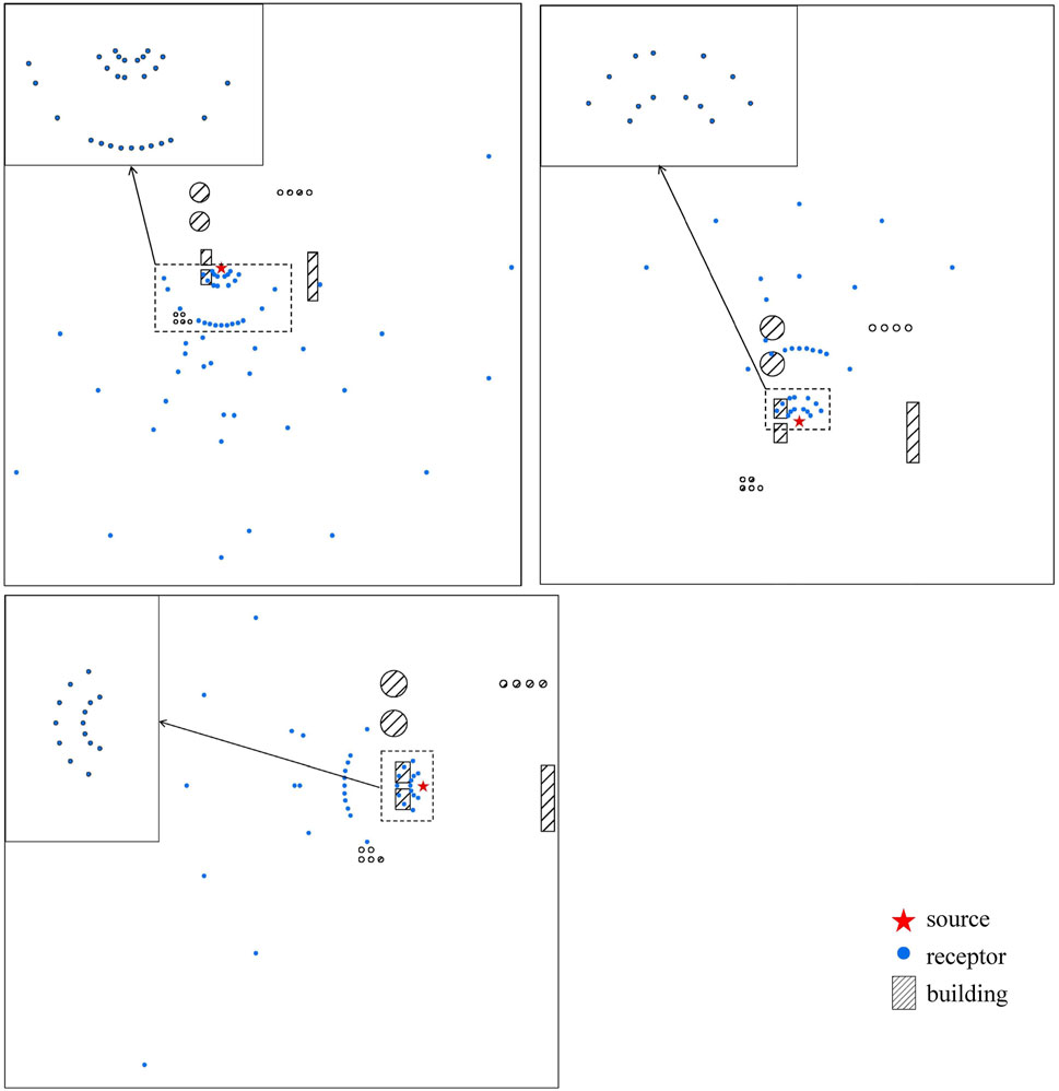
FIGURE 4. Map of measurement points and buildings in the base.

3.2 Wind tunnel experiments

The direct-current down-blowing wind tunnel used in this experiment consists of an inlet section, a drive section, a settling chamber, a contraction section, a test section, and an exhaust section. During the experiment, the airflow flows into the air inlet straightly and passes through the aforementioned sections in sequence and finally flows out of the air outlet. The miniature model of the base is placed in the wind tunnel, and the wind field conditions can be changed through the operating system. The gas dispersion process in the miniature model can be observed and analyzed through the measurement system.

The overall external dimensions of the wind tunnel are 10.4 m × 11.2 m × 81.0 m (width × height × length). The size of the test section is 4 m × 3 m × 20 m (width × height × length). To eliminate the static pressure gradient along the tunnel axis caused by the thickening of the tunnel wall’s boundary layer, the two side walls have a divergence angle of 0.8° (upper and lower walls are horizontal with no divergence angle). The aerodynamic profile of the wind tunnel is shown in Figure 5A. In this study, three wind directions of north, south, and east and two wind speeds of 3 and 6 m/s are used to form six different sets of wind field conditions.

FIGURE 5

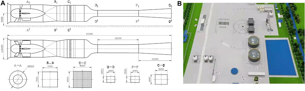
FIGURE 5. Models of the wind tunnel and experimental scene.(A) Design of the wind tunnel. (B) Physical miniature model.

In the experiment, ethylene (C₂H₄) is used as the tracer to simulate the diffusion of pollutants in the atmosphere. The gas flow rate is 200 ml/min. The initial ethylene concentration is 5 × 10⁵ ppm, and the concentration increases to 10⁶ ppm when the gas spreads over a distance of 300 mm.

We use a 1:300 scale experimental miniature model for the base surrounding area of 1 km, as shown in Figure 5B, which is placed in the test section of the wind tunnel in Figure 5A. A total of 128 concentration measurement points are set in the experiment, measuring the gas concentration at the height of 10 m in reality, some of which are evenly distributed around the pollution source in a circular ring, with the distances of 50, 100, 300, 900, and 1,500 mm from the pollution source, whose quantities are 16, 22, 38, 16, and 8, respectively. The others are distributed at densely populated and sensitive locations such as dormitories, office buildings, and equipment as supplementary, with the total number of 28.

3.3 Statistical evaluations

To evaluate the consistency of gas concentrations obtained from CALPUFF simulation and the wind tunnel experiment, we use the quantitative indexes proposed by (Hanna and Chang, 2012; Chang and Hanna, 2004),, which are the fractional bias (FB) and normalized mean square error (NMSE), defined as follows:

$\mathit{F}\mathit{B}=\frac{\mathbf{2}\left(\overline{{\mathit{X}}_{\mathit{o}}}-\overline{{\mathit{X}}_{\mathit{p}}}\right)}{\overline{{\mathit{X}}_{\mathit{o}}}+\overline{{\mathit{X}}_{\mathit{p}}}},(11)$

$\mathit{N}\mathit{M}\mathit{S}\mathit{E}=\frac{\overline{{\left({\mathit{X}}_{\mathit{o}}-{\mathit{X}}_{\mathit{p}}\right)}^{\mathbf{2}}}}{\overline{{\mathit{X}}_{\mathit{o}}}\overline{{\mathit{X}}_{\mathit{p}}}},(12)$

where the subscript P represents the CALPUFF model simulation result, O represents wind tunnel experiment observation, and $\overline{X_p}$ and $\overline{X_o}$ are the average values of the sampling points. FB and NMSE indexes can reflect the systematic deviation of the total data. In the most ideal scenario, that is, when the model result is completely consistent with the experimental results, both FB and NMSE are equal to 0.

Hanna and Chang also give the reference range of each index according to the characteristics of gas dispersion in urban areas: when |FB| ≤ 0.67 and NMSE ≤ 6, it indicates that the two sets of data fit well.

In addition, we also select the correlation coefficient R to reflect the correlation between two sets of data. If the |R| value is closer to 1, the linear correlation between the two sets of data is higher and vice versa.

$\mathit{R}=\frac{\overline{\left({\mathit{X}}_{\mathit{o}}-\overline{{\mathit{X}}_{\mathit{o}}}\right)\left({\mathit{X}}_{\mathit{p}}-\overline{{\mathit{X}}_{\mathit{p}}}\right)}}{{\mathit{\sigma }}_{\mathit{o}}{\mathit{\sigma }}_{\mathit{p}}},(13)$

where σ_o and σ_p are the standard deviations of the sampling points by CALPUFF model simulation and wind tunnel observation, respectively, and the meanings of other symbols are the same as before.

In the wind tunnel and CALPUFF experiments, the initial gas concentrations are c_0m and c_0p, and the gas concentrations at each measurement point are c_m and c_p, respectively. Gas concentrations obtained from the wind tunnel experiment and CALPUFF simulation cannot be directly compared. Therefore, we calculate the gas concentration dilution ratio for comparison, which is defined as follows:

$r_m=\frac{c_m}{c_{0m}},(14)$

$r_p=\frac{c_p}{c_{0p}}.(15)$

At the same measurement point, if r_m and r_p are close, they are consistent with each other, illustrating that they represent a similar diffusion process.

4 Results and discussion

In wind tunnel experiments, it is difficult to avoid the existence of background values, systematic errors, and random errors, leading to outliers and deviations. First, the records of wind tunnel experiments and CALPUFF calculation results are compared with themselves to eliminate the background value. Then, scatter fitting is performed on the remaining measurement points under each wind direction and speed, and the measurement points are divided into two groups in the near field and far field of the pollution source. The scatter plots are shown, respectively, in Figure 6. The points located 100 mm farther from the pollution source (corresponding to 30 m in reality) are designated as far-field measurement points, whose initial emission concentration of ethylene is 10⁶ ppm; and those within 100 mm are designated as near-field measurement points, with the initial emission concentration of 5 × 10⁵ ppm.

FIGURE 6

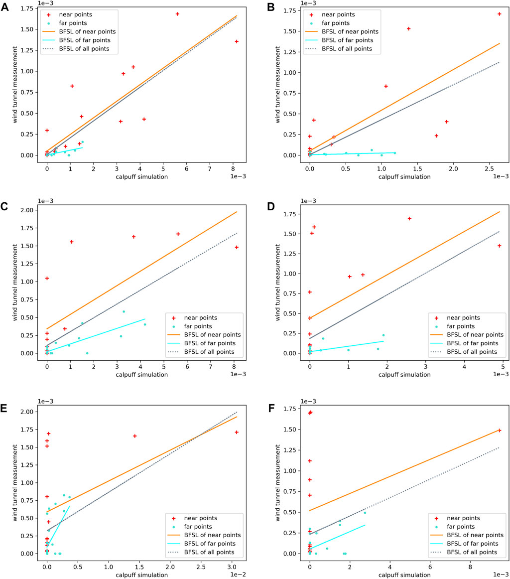
FIGURE 6. Scatter plots for the gas concentration dilution ratio of wind tunnel observation and CALPUFF simulation results: (A) N direction, 3 m/s, (B) N direction, 6 m/s, (C) S direction, 3 m/s, (D) S direction, 6 m/s, (E) E direction, 3 m/s, and (F) E direction, 6 m/s.

On the scatter plots, it can be found that the concentration distributions of measurement points in the near-field and far-field show different patterns. We use the best fit straight line (BFSL) to show the linear relationship of CALPUFF simulation and wind tunnel experiment results based on the least-squares estimation method.

As shown in Figures 6A–D, in the south and north wind directions, the slope of the BFSL of the far-field measurement points (blue line) is smaller than that of the near-field measurement points (orange line), which means CALPUFF tends to output higher gas concentration values in the far field than in the near field. The dilution effect of gas at far-field measurement points is more significant, leading to a smaller gas concentration dilution ratio, so the far-field scatter points are gathered near the origin of the coordinates. However, the distribution of near-field measurement points is more scattered, with a larger gas concentration dilution ratio, so the trend of BFSL of all measurement points is more significantly affected by the near-field measurement points. However, in the east wind direction, as shown in Figures 6E,F, contrary to the other wind directions, the slope of the blue line is larger than that of the orange line, which means that CALPUFF tends to output higher gas concentration values in the near field than in the far field. Also, the CALPUFF simulation results of the near-field points show little diversity, mostly clustered near the y-axis, so the trend of the BFSL of all measurement points is more significantly affected by the far-field measurement points. At the same time, it also shows that under east wind, due to the shielding of nearby buildings, gas dispersion is disturbed by a turbulent flow and the regularity of the spatial distribution of the gas concentration is not consistent, showing a more chaotic scatter distribution.

In order to further describe the continuous diffusion trend of polluted gas on the terrain surface, gridded receptors are set in CALPUFF to simulate the gas concentration on the surface layer. The result is overlaid with the concentration dilution ratio of the measurement points in the wind tunnel experiment, visually compared by means of graded coloring, as shown in Figure 7.

FIGURE 7

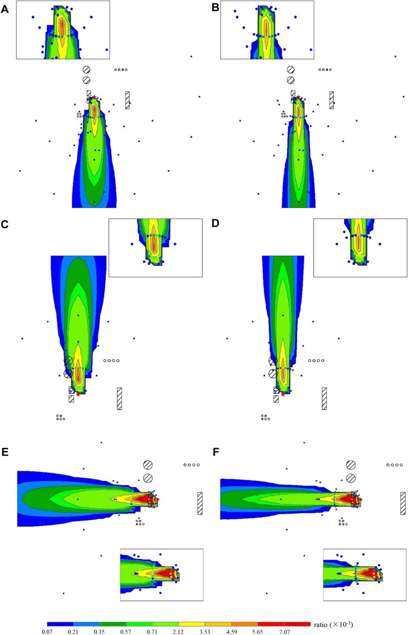
FIGURE 7. Overlaid comparison diagrams of wind tunnel observation and CALPUFF simulation results: (A) N direction, 3 m/s, (B) N direction, 6 m/s, (C) S direction, 3 m/s, (D) S direction, 6 m/s, (E) E direction, 3 m/s, and (F) E direction, 6 m/s.

Gas concentrations on the earth surface under different wind directions and speeds generally present the similar trend, which is gradually decreasing from the pollution source, and the simulation results show the best consistency with measurement points in the medium-level concentration (0.35 × 10⁻³ < ratio <3.53 × 10⁻³ in Figure 7). In addition, with larger wind speed, the horizontal diffusion range of the gas becomes smaller and the propagation distance becomes longer. Therefore, the shape of gas dispersion under the 6 m/s wind condition is narrower and sharper, and the concentration grades change more abruptly.

Under south and north wind directions, as shown in Figures 7A–D, the buildings are parallel to the wind directions, with heights of about 10 m and medium volumes, and the distance between the east and west buildings is about 160 m in reality, which is relatively large, so the diffusion of gas is less hindered by the surroundings. It can be observed that the horizontal distribution of the pollutant concentration is almost symmetrical, and the dilution effect in the downwind direction is smooth. Comparing the measurement points of the wind tunnel experiment and the CALPUFF simulation results of the surface layer, it is shown that their distribution trends are consistent, but the gas dilutes faster in the wind tunnel experiment. The measurement results of the wind tunnel experiment are all smaller than CALPUFF simulation results at the same location, so the diffusion range of the wind tunnel experiment is also smaller.

Under east wind, as shown in Figures 7E,F, an obvious high concentration center appears near the pollution source, covering a large area compared with other wind directions. Two buildings are distributed about 15 m from the pollution source on the leeward side by side and produce a complex turbulence. Relevant studies have shown that when the airflow passes through an area between the windward side and the leeward side that is equivalent to a “door hole,” the airflow accelerates. Also, when the “door hole” shrinks, the airflow speed increases. When the airflow passes buildings, positive pressure will be generated in the windward area and negative pressure will be generated in the side area. The pattern of pollutant concentration distribution is mainly affected by the turbulence. Where the turbulence is severer, the transportation of pollutants is easier to be transported in and out. Where the airflow is more stable, pollutants are harder to be transported to, but once they arrive, an area with high gas concentration may be generated after a period of accumulation (Zhuang, 2014). According to the distribution of results of the CALPUFF surface layer, a high concentration center forms behind the near-field buildings, showing that along the leeward direction from the pollution source, the pollutant concentration first increases and reaches the peak concentration behind the buildings on the midline of the two buildings and then gradually dilutes. This may be due to the fact that the east wind in the experiment accelerates and transports a large amount of pollutants when passing through the two buildings in the near field, which deposit and accumulate around the buildings due to the stable airflow. Comparing the CALPUFF dispersion result with the measurement points in the wind tunnel experiment, both the magnitude and distribution trend of the concentration dilution ratio fit well.

In order to quantitatively compare the results of the two methods, for the far- and near-field measurement points under different wind directions and speeds, the results of the evaluation indexes in 3.3 are shown in Table 2.

TABLE 2

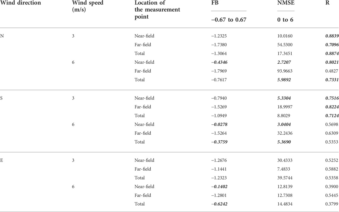
TABLE 2. Evaluation indexes for the comparison of the wind tunnel experiment and CALPUFF simulation under different wind directions and speeds.

For the FB and NMSE indexes used in this study, the smaller the value, the better is the consistency of the two groups of data. The FBs and NMSEs in Table 2 within the reference range in 3.3 are bold and italic. For the R index, generally, the R value between 0 and 0.3 indicates a weak positive linear relationship; the value between 0.3 and 0.7 indicates a moderate positive linear relationship; and the value between 0.7 and 1 indicates a strong positive linear relationship (Ratner, 2009). The Rs in Table 2 all exceed 0.3, and the Rs over 0.7 are bold and italic.

From the perspective of FBs and NMSEs, in the four groups of experiments under south and north wind, the order of absolute values is as follows: near field < total < far field. For example, under north wind with the speed of 6 m/s, the order of FBs is |−0.4346| < |−0.7617| < |−1.7969|; and under south wind with the speed of 3 m/s, the order of NMSEs is |5.3304| < |8.8029| < |18.9997|. It reveals that for the magnitude of the results, the simulation accuracy is the highest of the near-field measurement points but the lowest of the far-field measurement points. Under east wind, there is no such regularity of the order of values, but the results of 6 m/s show better indexes than 3 m/s, with lower FBs and NMSEs in most cases.

From the perspective of the R index, under north wind, the order of values is near field > far field, and the near-field values are over 0.8. For example, the Rs’ order of near-field and far-field points under 3 m/s is 0.8839 >0.7096; and under 6 m/s is 0.8021 >0.4827. It illustrates that CALPUFF simulates the concentration distribution in near field well and has the ability to reflect the diffusion regularity of pollutants in space. Under both south and east wind, the orders of Rs are as follows: far field > near field. For example, under south wind with the speed of 3 m/s, the order of far-field and near-field points is 0.8224 > 0.7516. It indicates that CALPUFF simulates better in the far field. However, under east wind, Rs of near-field points are only about 0.4, showing more difficulty and uncertainty for both CALPUFF simulation and the wind tunnel experiment caused by complex buildings.

In addition, from the perspective of different wind speeds, under south and north wind, the performances of the evaluation indexes under the wind speed of 3 m/s are better than those of 6 m/s. Because the higher the wind speed, the more unstable is the airflow, causing more difficulty in data collection, and the credibility of the observations in the wind tunnel experiment may decrease.

5 Conclusion

In this study, a wind tunnel experiment and a CALPUFF simulation experiment of the ethylene gas leakage accident are designed and implemented for a national hazardous chemicals emergency rescue base, with a total of six groups of experimental conditions under three wind directions and two wind speeds. The experiment results of each group are, on one hand, qualitatively compared by visualization methods such as scatter plots and overlay analysis and, on the other hand, quantitatively compared by FB, NMSE, and R indexes, in order to analyze the differences between the results of the two methods. This study leads to the following conclusions:

(1) Generally, the CALPUFF model can simulate the diffusion trend of pollution gas accurately, reflecting the regularity of its spread in space, but in the aspect of magnitude of the results, CALPUFF tends to underestimate the concentration in the near field of the pollution source and overestimate the concentration in the far field.

(2) The CALPUFF model has very limited capabilities of processing the scenes with complex buildings (such as urban environments). Airflow near buildings is fickle, especially when the pollution source is located very close to buildings, leading to inaccurate results.

(3) In wind tunnel experiments, many steps are operated artificially, such as the manufacture of physical models, adjustment of gas emission, and layout of measurement points, which are significantly affected by the experimenters’ working ability. They may also lead to deviations in the results, so the measurement points with a poor reference can be filtered and excluded in advance of the analysis. Additionally, extra measurement points can be added at some important locations such as front and behind the near-field buildings, according to specific conditions, so as to inspect the changes in the pollutant diffusion process subtly.

Based on the aforementioned analysis and conclusions, both the wind tunnel experiment and CALPUFF model are important means of simulating gas leakage accidents currently, with their own advantages and disadvantages. The wind tunnel experiment can recur the real scene as more as possible and has lower cost and fewer restrictions than traditional field measurements, so it is more applicable to complex surface conditions and crowded environments, but it also requires more accurate measurement devices and higher ability of experimenters, with more complicacy of error analysis. The CALPUFF model is more convenient to use and can repeatedly adjust and test different experimental parameters with satisfactory accuracy for general emergency plans’ requirement. However, the simulation result of CALPUFF is not good enough for fine-scale and complex near-field environments. In future studies, researchers can work on improving the building module of the gas dispersion model to improve its simulation accuracy. Also, more precise equipment and comprehensive solutions can be used in the wind tunnel experiment to improve its reliability. The simulation results of gas leakage accidents should be selectively referred to: if the case is in the near-field area of the pollution source significantly affected by buildings, the wind tunnel experiment is a better reference, but if the case is in the far-field and relatively open area, as well as to simulate an overall concentration distribution, CALPUFF can also provide a more credible reference.

Data availability statement

The raw data supporting the conclusion of this article will be made available by the authors, without undue reservation.

Author contributions

RZ: conceptualization, methodology, validation, and writing—original draft. ML: conceptualization and writing—review and editing. HM: writing—review and editing.

Conflict of interest

The authors declare that the research was conducted in the absence of any commercial or financial relationships that could be construed as a potential conflict of interest.

Publisher’s note

All claims expressed in this article are solely those of the authors and do not necessarily represent those of their affiliated organizations, or those of the publisher, the editors, and the reviewers. Any product that may be evaluated in this article, or claim that may be made by its manufacturer, is not guaranteed or endorsed by the publisher.

References

AERMOD, (2019). User's Guide for the AMS/EPA Regulatory Model (AERMOD) [DB/OL]. United States: U.S. Environmental Protection Agency

Google Scholar

Carruthers, D. J., Holroy, D. R. J., Hunt, J. C. R., Weng, W. S., Robins, A. G., Apsley, D. D., et al. (1994). UK-ADMS: A new approach to modelling dispersion in the earth's atmospheric boundary layer. J. Wind Eng. Industrial Aerodynamics 5 (52), 139–153. doi:10.1016/0167-6105(94)90044-2

CrossRef Full Text | Google Scholar

Chang, J. C., and Hanna, S. R. (2004). Air quality model performance evaluation. Meteorol. Atmos. Phys. 87 (1-3), 167–196. doi:10.1007/s00703-003-0070-7

CrossRef Full Text | Google Scholar

Cheng, K., Zhao, X., Zhou, W., Cao, Y., Yang, S. H., and Chen, J. (2021). Source term estimation with deficient sensors: Traceability and an equivalent source approach. Process Saf. Environ. Prot. 152, 131–139. doi:10.1016/j.psep.2021.05.035

CrossRef Full Text | Google Scholar

Cimorelli, A. J., Perry, S. G., Venkatram, A., Weil, J. C., Paine, R. J., Wilson, R. B., et al. (2004). Aermod – description of model formulation. Research Triangle Park, North Carolina: U.S. Environmental Protection Agency

Google Scholar

Dong, X., Zhuang, S., Fang, S., Li, H., and Cao, J. (2021). Site-targeted evaluation of SWIFT-RIMPUFF for local-scale air dispersion modeling around Sanmen nuclear power plant based on multi-scenario wind tunnel experiments. Ann. Nucl. Energy 164, 108593. doi:10.1016/j.anucene.2021.108593

CrossRef Full Text | Google Scholar

Fallah Shorshani, M., Seigneur, S., Rehn, P., and Chanut, D. (2015). Atmospheric dispersion modeling near a roadway under calm meteorological conditions. Transp. Res. Part D Transp. Environ. 34, 137–154. doi:10.1016/j.trd.2014.10.013

CrossRef Full Text | Google Scholar

Fallah-Shorshani, M., Shekarrizfard, M., and Hatzopoulou, M. (2017). Integrating a street-canyon model with a regional Gaussian dispersion model for improved characterisation of near-road air pollution. Atmos. Environ. 153, 21–31. doi:10.1016/j.atmosenv.2017.01.006

CrossRef Full Text | Google Scholar

Hanna, S., and Chang, J. (2012). Acceptance criteria for urban dispersion model evaluation. Meteorol. Atmos. Phys. 116 (3-4), 133–146. doi:10.1007/s00703-011-0177-1

CrossRef Full Text | Google Scholar

Holmes, N. S., and Morawska, L. (2006). A review of dispersion modelling and its application to the dispersion of particles: An overview of different dispersion models available. Atmos. Environ. 40 (30), 5902–5928. doi:10.1016/j.atmosenv.2006.06.003

CrossRef Full Text | Google Scholar

Holnicki, P., Kałuszko, A., and Trapp, W. (2016). An urban scale application and validation of the calpuff model. Atmos. Pollut. Res. 7 (3), 393–402. doi:10.1016/j.apr.2015.10.016

CrossRef Full Text | Google Scholar

Huang, Z., Yu, Q., Ma, W., and Chen, L. (2019). Surveillance efficiency evaluation of air quality monitoring networks for air pollution episodes in industrial parks: Pollution detection and source identification. Atmos. Environ. 215, 116874. doi:10.1016/j.atmosenv.2019.11687410

CrossRef Full Text | Google Scholar

Huber, A. H., and Synder, W. H. (1976). “Building wake effects on short stack effluents,” in Proceedings of the Preprint volume for the third symposium on atmospheric diffusion and air quality (Boston, Massachusetts: American Meteorological Society).

Google Scholar

Huber, A. H. (1977). “Incorporating building/terrain wake effects on stack effluents,” in Proceedings of the Preprint volume for the joint conference on applications of air pollution meteorology (Boston, Massachusetts: American Meteorological Society).

Google Scholar

Jiang, X., Yang, H., Lin, G., Dang, W., Xin, B., Zhang, J., et al. (2021). Measurements and predictions of harmful releases of the gathering station over the mountainous terrain. J. Loss Prev. Process Industries 71 (8), 104485. doi:10.1016/j.jlp.2021.104485

CrossRef Full Text | Google Scholar

Jones, A., Thomson, D., Hort, M., and Devenish, B. (2007). “The U.K. Met office's next-generation atmospheric dispersion model, NAME III,” in Air pollution modeling and its application XVII. Editors C. Borrego, and A. L. Norman (Boston, MA: Springer). doi:10.1007/978-0-387-68854-1_62

CrossRef Full Text | Google Scholar

Kota, S. H., Qi, Y., and Zhang, Y. (2013). Simulating near-road reactive dispersion of gaseous air pollutants using a three-dimensional Eulerian model. Sci. Total Environ. 454-455 (1), 348–357. doi:10.1016/j.scitotenv.2013.03.039

PubMed Abstract | CrossRef Full Text | Google Scholar

Li, K., Liang, M., and Su, G. (2018). Data assimilation method for atmospheric dispersion based on a Gaussian puff model. J. Tsinghua Univ. Technol. 58 (11), 992–999. doi:10.16511/j.cnki.qhdxxb.2018.22.049

CrossRef Full Text | Google Scholar

Li, M., Yang, D., and He, W. (2020). Comparison and perspective on theories and simulation results of gas dispersion models AERMOD and CALPUFF. Geomatics Inf. Sci. Wuhan Univ. 45 (08), 1245–1254. doi:10.13203/j.whugis20200110

CrossRef Full Text | Google Scholar

Liu, Y., Li, H., Sun, S., and Fang, S. (2017). Enhanced air dispersion modelling at a typical Chinese nuclear power plant site: Coupling RIMPUFF with two advanced diagnostic wind models. J. Environ. Radioact. 175/176, 94–104. doi:10.1016/j.jenvrad.2017.04.016

PubMed Abstract | CrossRef Full Text | Google Scholar

Ministry of Ecology and Environment of the People’s Republic of China (2018). Technical Guidelines for environmental impact assessment—atmospheric Environment HJ 2.2-2018. https://www.mee.gov.cn/ywgz/fgbz/bz/bzwb/other/pjjsdz/201808/W020180814672740551977.pdf

Google Scholar

Mishra, K. B., and Wehrstedt, K. D. (2015). Underground gas pipeline explosion and fire: CFD based assessment of foreseeability. J. Nat. Gas Sci. Eng. 24, 526–542. doi:10.1016/j.jngse.2015.04.010

CrossRef Full Text | Google Scholar

NOAA and EPA (2007). ALOHA user's manual. February, 2007. Retrieved from: https://nepis.epa.gov/Exe/ZyPDF.cgi/P1003UZB.PDF?Dockey=P1003UZB.PDF

Google Scholar

Ratner, B. (2009). The correlation coefficient: Its values range between +1/1, or do they? J. Target. Meas. Anal. Mark. 17 (2), 139–142. doi:10.1057/jt.2009.5

CrossRef Full Text | Google Scholar

Ridzuan, N., Ujang, U., Azri, S., and Choon, T. L. (2020). Visualising urban air quality using AERMOD, CALPUFF and CFD models: A critical review The International Archives of the Photogrammetry, Remote Sensing and Spatial Information Sciences. XLIV-4/W3-2020, 355–363. doi:10.5194/isprs-archives-xliv-4-w3-2020-355-2020

CrossRef Full Text | Google Scholar

Rood, A. S. (2014). Performance evaluation of AERMOD, CALPUFF, and legacy air dispersion models using the Winter Validation Tracer Study dataset. Atmos. Environ. 89 (2), 707–720. doi:10.1016/j.atmosenv.2014.02.054

CrossRef Full Text | Google Scholar

Rzeszutek, M. (2019). Parameterization and evaluation of the calmet/calpuff model system in near-field and complex terrain-terrain data, grid resolution and terrain adjustment method. Sci. Total Environ. 689 (1), 31–46. doi:10.1016/j.scitotenv.2019.06.379

PubMed Abstract | CrossRef Full Text | Google Scholar

Schulman, L. L., and Hanna, S. (1986). Evaluation of downwash modifications to the industrial source complex model. J. Air Pollut. Control Assoc. 36, 258–264. doi:10.1080/00022470.1986.10466066

CrossRef Full Text | Google Scholar

Schulman, L. L., and Scire, J. S. (1980). Buoyant line and point source (BLP) dispersion model user's guide. Final report.Available at: https://www.osti.gov/biblio/5824114

Google Scholar

Scire, J. S., Strimaitis, D. G., and Yamartino, R. J. (2011). A user's guide for the Calpuff dispersion model. Available at: http://www.src.com/calpuff/download/CALPUFF_UsersGuide.pdf

Google Scholar

Stein, A. F., Draxler, R. R., Rolph, G. D., Stunder, B. J. B., Cohen, M. D., and Ngan, F. (2016). NOAA’s HYSPLIT atmospheric transport and dispersion modeling system. Bull. Am. Meteorol. Soc. 96, 2059–2077. doi:10.1175/BAMS-D-14-00110.1

CrossRef Full Text | Google Scholar

Stockie, J. M. (2011). The mathematics of atmospheric dispersion modeling. SIAM Rev. Soc. Ind. Appl. Math. 53 (2), 349–372. doi:10.1137/10080991x

CrossRef Full Text | Google Scholar

Toscano, D., Marro, M., Mele, B., Murena, F., and Salizzoni, P. (2021). Assessment of the impact of gaseous ship emissions in ports using physical and numerical models: The case of Naples. Build. Environ. 196, 107812. doi:10.1016/j.buildenv.2021.107812

CrossRef Full Text | Google Scholar

Ulimoen, M., Berge, E., Klein, H., Salbu, B., and Lind, O. C. (2022). Comparing model skills for deterministic versus ensemble dispersion modelling: The fukushima daiichi npp accident as a case study. Sci. Total Environ. 806, 150128. doi:10.1016/j.scitotenv.2021.150128

PubMed Abstract | CrossRef Full Text | Google Scholar

Yan, X., Guo, X., Liu, Z., and Yu, J. (2016). Release and dispersion behaviour of carbon dioxide released from a small-scale underground pipeline. J. Loss Prev. Process Industries 43, 165–173. doi:10.1016/j.jlp.2016.05.016

CrossRef Full Text | Google Scholar

Yassin, M. F., Alhajeri, N. S., Elmi, A. A., Malek, M. J., and Shalash, M. (2021). Numerical simulation of gas dispersion from rooftop stacks on buildings in urban environments under changes in atmospheric thermal stability. Environ. Monit. Assess. 193 (1), 22. doi:10.1007/s10661-020-08798-x

PubMed Abstract | CrossRef Full Text | Google Scholar

Yu, X., and Cao, L. (2020). A review of the Lagrangian diffusion model for atmospheric pollution. Environ. Eng. 38 (09), 145–153. doi:10.13205/j.hjgc.202009024

CrossRef Full Text | Google Scholar

Yuan, D., Li, S., Huang, Y., and Wu, M. (2013). Research progress on diffusion model of petrochemical industry gas leakage. Energy Chem. Ind. 34 (02), 21–26. doi:10.3969/j.issn.1006-7906.2013.02.006

CrossRef Full Text | Google Scholar

Zhuang, S. (2014). Study on mechanism of gas flow and pollutant dispersion around the buildings. PhD thesis. Shenyang (IL): Northeastern University (Chinese).

Google Scholar