Predicting wine prices based on the weather: Bordeaux vineyards in a changing climate

Each grapevine cultivar needs a certain amount of cumulated heat over its growing season for its grapes to ripen properly. In the 20th century’s Bordeaux vineyard, the average growing season temperature was not always sufficient, thus higher than usual summer temperatures were on average linked with higher grape and wine quality. However, over the last 60+ years, global warming gradually increased the vineyard’s temperatures up to the point where additional growing season heat is not required anymore, and can even become detrimental to wine quality: hence the positive effect of higher-than-usual summer temperatures has progressively vanished. In this context, it is unknown whether any weather variable is still a good predictor of a vintage’s quality. Here we provide a predictive model of wine prices, based only on weather data. We establish that it predicts a vintage’s long-term quality more accurately than a world-class expert rating this same vintage in the year following its production. We first design a corpus of features suited to the grapevine lifecycle to extract from them the most powerful drivers of wine quality. We then build a predictive model that leverages Local Least Squares kernel regression (LLS) to factor in the time-varying nature of climate impact on the grapevine. Hence, it is able to outperform previous models and even provides a better predictive ranking of successive vintages than the grades given by world-famous wine critic Robert Parker. This predictive power demonstrates that weather is still a very efficient predictor of wine quality in Bordeaux. The two main features on which this model is built—following grapevine’s phenological calendar and using an LLS architecture to let the input-output relationship vary over time—could help model other agricultural systems amidst climate change and adaptation of production processes.

1 Introduction

Viticulture is particularly sensitive to the effect of climate, as the weather has been ranked as a better explanatory variable of grape quality variations than soil or grape variety (van Leeuwen et al., 2004). The effects of individual weather variables on grape—and thus wine quality, have been subject to many attempts of quantification, particularly so in Bordeaux (France) where researchers can draw on an abundant corpus of data. The average temperature during the grapevine (Vitis vinifera) growing season, from April to September, has been identified as the main driver of wine quality in Bordeaux before the year 2000 (Jones and Davis, 2000; Ashenfelter, 2008), as is the case in other regions (Byron and Ashenfelter, 1995; Haeger and Storchmann, 2006; Corsi and Ashenfelter, 2019; Biss and Ellis, 2021). Indeed, low temperatures are linked with low sugar levels, which often coincide with poor vintage ratings in Bordeaux (Gambetta and Kurtural, 2021). Thus we could talk about a lower temperature threshold for vinegrowing. This threshold has been overcome in Bordeaux by the substantial warming of the last 60 + years, and the average growing season drew closer to an optimum where vintage qualities would be more consistently good. But further warming increases the frequency of very high temperatures that can have deleterious effects on wine grape composition, including decreases in anthocyanins (Gambetta and Kurtural, 2021), molecules that enhance wine color and ageing capacity (Pérez-Magariño and González-San José, 2006). Hence, some consider that quality in Bordeaux has reached a plateau (Gambetta and Kurtural, 2021). As a result, Almaraz (2015) provided statistical evidence that over the last decades, average growing season temperature has lost a major part of its explanatory power for wine quality in Bordeaux. The question is thus still open, whether a vintage’s weather is still a strong determinant of the quality of Bordeaux wine or not.

But how should wine quality be measured? Prices and critical ratings are the two main proxies of quality. The 1855 Bordeaux ranking classified the Grands crus according to their average price (Ashenfelter, 2008). In the scientific literature, quality has been alternatively measured through auction prices (e.g. Jones and Storchmann, 2001; Jones et al., 2005; Haeger and Storchmann, 2006) or critical ratings (e.g. Baciocco et al., 2014; Almaraz, 2015). The system of primeur, used for two centuries as the main route to market for Bordeaux premium wines, is the first way of aligning prices, ratings, and long-term quality: in April following the year of production, wine is tasted in its prime—thus the word primeur- and the barrels of future wine are bought by traders long before the end of the production process. At that time, the young Bordeaux Grands crus are typically too tannic and have not reached their optimal taste (Jones and Storchmann, 2001), thus their true, long-term quality is unknown. Therefore, there is a gap between short and long-term prices, which can be exploited with additional information. This is why critical grades published by experts at primeurs, although they are only a temporary evaluation of a vintage’s future quality, have a strong impact on the price, as evidenced by Ali et al. (2008). Then over the next decade, owing to the ageing of wine which progressively reveals its quality, prices and ratings partially realign towards the true long-term quality, for instance through auction sales where demand regulates price (Storchmann, 2012). In this study, we show that quantitative models based on a vintage’s weather can provide more reliable information about its quality than primeur critical grades. First, despite the decline of the average temperature as a predictor of wine quality, we show that other weather parameters are meaningful enough to have a quantifiable impact on long-term prices. Based on these predictors, we then develop a model for the prediction of long-term prices of vintages. This model achieves state-of-the-art predictive performance and even beats the predictive accuracy of early critical grades.

2 Materials and methods

2.1 Data collection

2.1.1 Selecting a corpus of study

Roberts and Reagans (2007) show that the more a particular wine is exposed to critical ratings, the steeper the relationship between ratings and prices is; which we interpret as a stronger relationship between prices and quality: following this logic, our corpus of study consists of top Bordeaux wines. The sources used for selecting these wines were the 1855 ranking, the Graves ranking, the Saint-Emilion ranking, and prices for Pomerol wines. As the winemaking process differs between red and white wines, considering that more of the former are included in the different rankings across Bordeaux, the corpus was restricted to red wines. Finally, to reduce the price variability due to very localized events such as hail, only vineyards above areas of 5 ha were included in the corpus. The resulting corpus includes 59 different Bordeaux red wines, which belong to four Appellations d’Origine Contrôlée, henceforth named appellations. The complete list can be found in the Supplementary Appendix Table S1, and it is represented in Figure 1.

FIGURE 1

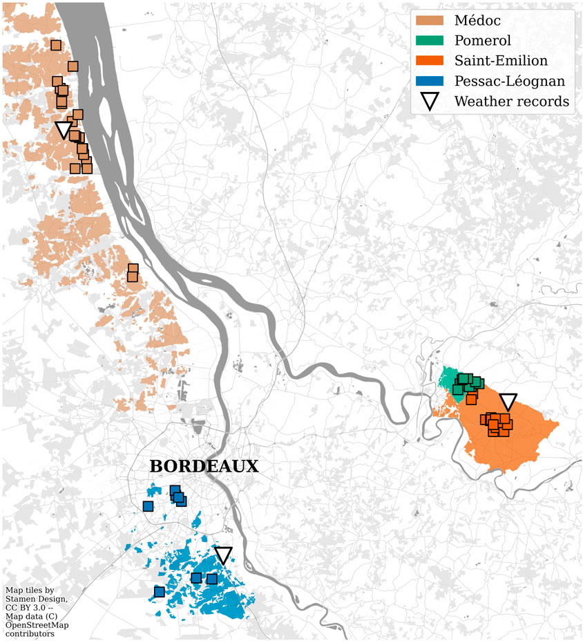
FIGURE 1. Map of selected vineyards. Squares are individual vineyards, color areas are the appellations.

2.1.2 Long-term wine prices

The long-term auction prices for 59 Bordeaux red wines over 53 different vintages were collected from the auction website IDealwine¹, which provides an index of average prices from the last auction sales. The data collection starts from vintage 1960, at which price records are available for a large majority of wines, and it ends at vintage 2013. The wines with more than five missing entries since 1960 were removed from the lists, leaving a total of 39 wines (see Supplementary Appendix Table S1). These prices will be our representation of the bottle’s long-term prices since each price point is an actualized price for a vintage over 9 years old. Figure 2 displays the evolution of average bottle prices over all vineyards of the four appellations.

FIGURE 2

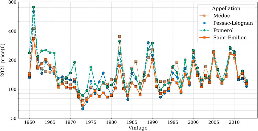
FIGURE 2. Evolution of average bottle prices for the four appellations for vintages 1960–2013. Y-scale is logarithmic.

2.1.3 Vinegrowing calendar data

Following Jones and Davis (2000), each vintage was divided according to the different phenological events, which are the milestones of the grape’s development. Indeed, the same weather condition can have a different impact on the grapevine depending on its growth phase, which can be captured only when partitioning the calendar in a physiologically relevant way. The most important phenological events, given here with their code on the BBCH scale (Lancashire et al., 1991) are budbreak (BBCH 07), flowering (BBCH 65), véraison (BBCH 85, the onset of ripening, marked by the changing of color of the grapes). These events can occur earlier or later across different Bordeaux appellations or for different grapevine varieties (e.g. Merlot is generally earlier than Cabernet), so the records obtained mention approximate dates. Even though the harvest is not a phenological event, harvest dates have also been included in the calendar, because they mark the end of the climate’s impact on the grapes. These historical dates were compiled from the records of Château Latour and the University of Bordeaux, to establish an approximate calendar of phenological events spanning the timeframe 1960–2017 (Table 1 and Figure 3).

TABLE 1

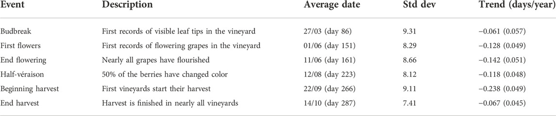
TABLE 1. Vinegrowing calendar, from 1960 to 2017.

FIGURE 3

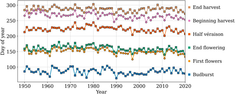
FIGURE 3. Vinegrowing calendar.

The phenological events of each vintage provide a natural partition of the growing season in specific intervals:

• Budbreak—flowering: from budbreak to the first flowers

• Flowering: from the first flowers to the complete flowering

• Flowering—véraison: from the complete flowering to half-véraison

• Véraison—harvest: from half-véraison to the beginning of the first harvests

• Harvest: from the beginning of the first to the end of the last harvest

These intervals will be used to aggregate the weather data collected in the next subsection.

2.1.4 Weather data

The weather data was gathered from the SAFRAN reanalysis of Météo France (Vidal et al., 2010), available in 8 km grid points, with daily granularity since 1958. The vineyards of each appellation were assigned weather data from one grid point: Saint-Émilion (Lon: −0.14, Lat: 44.91), for the Saint-Emilion and Pomerol appellations, Pauillac (Lon: −0.767, Lat: 45.182) for Médoc, and Léognan (Lon: 0.542/Lat: 44.756) for Pessac-Léognan. The selected weather variables shown are of classical use in the literature as predictors of wine quality. Based on van Leeuwen and Darriet (2016) who showed a highly significant correlation between wine quality and water deficit, the variable Water Deficit (WD), is calculated based on the simplified grapevine transpiration formula (Riou et al., 1994):

$\mathrm{W}\mathrm{D}=\mathrm{k}*\mathrm{E}{\mathrm{T}}_0-\mathrm{P}(1)$

with $\mathrm{E}{\mathrm{T}}_0$ the Penman evapotranspiration, P the precipitations, and k = 0.3 from budbreak to flowering and 0.6 after flowering (van Leeuwen et al., 2004).

These weather parameters are then averaged over the five phenological intervals defined in the previous subsection to yield. Five different predictor features each. For instance, P (Precipitations) provides five different features: P: budbreak—flowering (average daily precipitations from budbreak to the beginning of flowering), P: flowering (average daily precipitations during flowering), P: flowering—véraison, etc. The same goes with all parameters of Table 2, except for Frost days: this parameter is not averaged over five phenological intervals but summed only over the phenological interval Budbreak—flowering.

TABLE 2

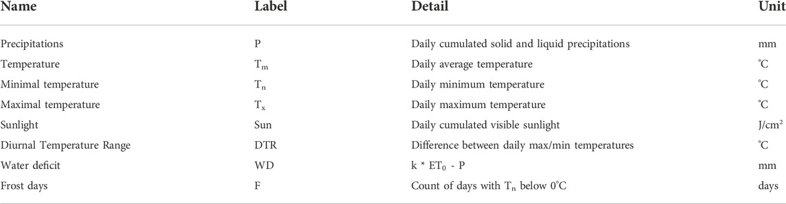
TABLE 2. Weather variables.

2.1.5 Critical grades

As an accuracy benchmark against which to compare our predictive model, we collect critical primeur grades. The most influential critic in recent decades was without a doubt Robert Parker. His primeur grades were collected for the vintages 1994 through 2013, for 19 vineyards (list in Supplementary Appendix Table S2). Hence, our models will be evaluated on vintages 1994 to 2013 (20 vintages). Provided the tasted wines were young and still poised to evolve, each grade was only given as an interval and updated later to a single grade: as the goal here is to provide a benchmark of predictive performance, a unique grade is created by averaging the lower and upper bounds.

On our corpus of wines, average Spearman correlations between ratings and 2022 prices exhibit an increase across vintages (Figure 4), which is confirmed by a Kendall-Tau test (trend: 0.179, p-value: 0.0002): this means that the correlation of prices with ratings is stronger for recent vintages. It could be that there is a recent trend of relying more on expert opinion. But this more likely suggests that ageing vintages progressively decorrelate in value from early ratings, which we attribute to the fact that wine reveals its true quality with age, as mentioned by Storchmann (2012). This impact on early prices, and ulterior partial decorrelation, tends to confirm the short-term self-fulfilling prophecy effect of ratings already described in the literature (Ali et al., 2008). This side effect arguably boosts the performance of critical grades for price prediction, making it harder for predictive models to compete.

FIGURE 4

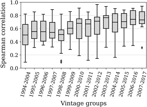
FIGURE 4. Spearman correlation between Wine Advocate primeur ratings and 2021 prices across vintage windows.

2.2 Predictive modeling

The goal of this part is to provide a predictive model of long-term wine prices.

2.2.1 Model evaluation: Log specification, ex-ante testing, and metrics

Literature on hedonic wine price functions generally recommends using the logarithm specification for the price (Oczkowski, 1994; Schamel and Anderson, 2003), which is supported by the better correlation of this specification with critical ratings (Oczkowski and Doucouliagos, 2015), hinting that it has a linearly more consistent variation with quality: as a result, the log specification is used hereafter. As our goal is to build a predictive model of wine prices, the real evaluation setting must be reproduced, in which the model must predict a previously unseen data point (here, the logarithm of a vintage’s price), and can only access data points from previous years. This is a case of ex-ante model testing, where the testing timeframe is posterior to the training timeframe, which prevents the model from accessing future trends during its training (Aristodemou and Tietze, 2018). Previous literature has only used in-sample testing instead to present their results (Jones and Davis, 2000; Jones and Storchmann, 2001; Jones et al., 2005; Ashenfelter, 2008; Baciocco et al., 2014; Corsi and Ashenfelter, 2019), meaning that the model was tested on the same data that it was trained on: this explains important performance gaps between their models’ results in this paper and previous evaluations. In the rest of this study, for the prediction of vintage v, each model is trained on a timeframe starting with the first available vintage (1960) and ending at vintage v-1, as displayed in Figure 5A. Each model is tested on the 1994–2013 time range (20 vintages), thus implying different training windows: for instance, vintage 1994 is predicted by models trained with the data from the years 1960–1993, and vintage 2004 is predicted based on the years 1960–2003. Evaluation metrics used are the Mean Absolute Error (MAE), the coefficient of determination, noted ${\mathrm{R}}^2$, and the Spearman rank correlation noted ρ_S (definitions can be found in the Supplementary Appendix Table S3). It is important to note that the coefficient of determination can be negative for all models in the setting of out-sample prediction, as mentioned e.g. by Chicco et al. (2021).

FIGURE 5

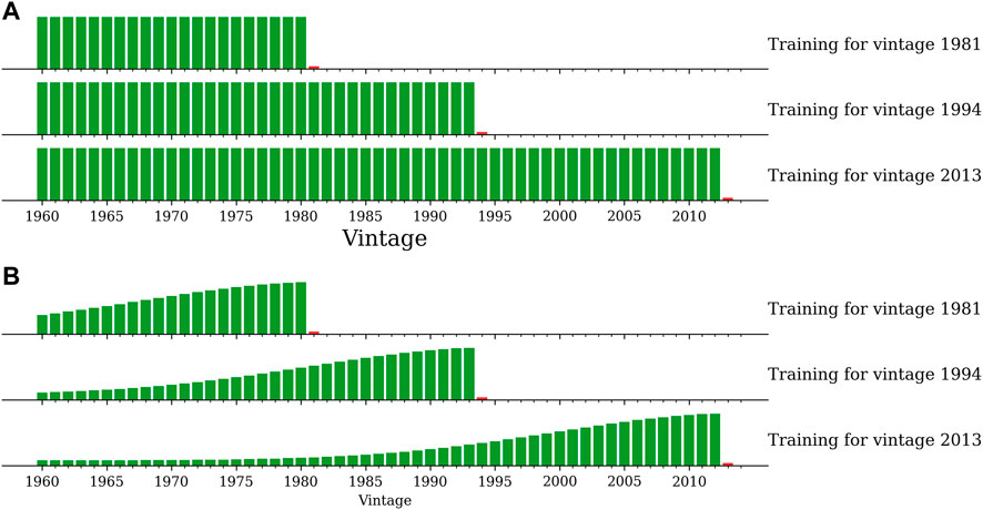
FIGURE 5. Intuition for the LLS model. Each line is a training setting for predicting the vintage marked as the small red bar. Relative weights of training data points are figured as green bars. (A) Equal weights for all training datapoints: OLS model. (B). High weight for recent vintages, low weights for older vintages: LLS model. The weights are determined by a kernel function.

2.2.2 Feature selection

This section aims at selecting, out of all weather variables built in Section 2.1, a set of the best predictors of wine quality. To this end, the available weather variables for all vineyards are normalized, then concatenated into one cross-vineyard ensemble. The same is done for prices, which allows to compute statistics between any weather variable and overall prices. The Pearson R correlation with prices is computed for all weather variables, and the strongest correlations in absolute value are displayed in Table 3.

TABLE 3

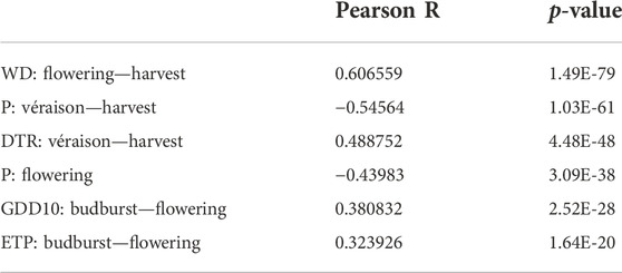
TABLE 3. Top weather variables ranked by absolute correlation with prices.

WD: flowering - harvest has the clearest correlation with prices. This is coherent with previous research where moderate water deficit is often associated with high-quality wine (Fraga et al., 2013; van Leeuwen and Darriet, 2016; Alem et al., 2019; Fayolle et al., 2019) because it leads to an increased grape tannin and anthocyanin content in various varieties (Duteau et al., 1981; Matthews and Anderson, 1988; van Leeuwen et al., 2009; Blank et al., 2019), as well as increased sugar concentration in fruit (Castellarin et al., 2007; Zsófi et al., 2011). Thus we will include this weather variable in our predictor set. The next most strongly correlated feature is P: véraison - harvest, which we will not consider for inclusion in our predictor set because it is too strongly correlated with WD: flowering—harvest (Pearson correlation: −0.75).

DTR: véraison - harvest has a strong positive correlation with prices. A high diurnal temperature range has already been linked to high quality (Gladstones 1992; cited in Jones et al., 2005), because it would be a sign of both a high diurnal temperature (crucial for berry ripening), and cool night temperatures enabling the production of the secondary metabolites associated with high-quality flavors (Tonietto and Carbonneau, 2004). However, this assertion has not been supported yet by any data, with some studies even concluding the opposite: it is therefore still debated to our knowledge (de Rességuier et al., 2020), and would necessitate further investigation to be a proven point. Nonetheless, as in the present case, the variable seems to have a strong positive impact on prices, it could have another relationship with prices, e.g. high DTR could only imply that the nights are cool, which could have a positive influence on quality. It will thus be used as a predictor of prices.

Finally, the negative correlation of P: flowering with prices makes sense. Flowering precipitations have been documented to cause climatic coulure and thus reduce yield (Blank et al., 2019). Prior literature displays little evidence of a reduction of quality, probably because an assessment of this impact is made more difficult by the lack of accessible phenology calendar data, but from our discussions with vintners in the Bordeaux area, the occurrence of strong rain during the flowering period is a very bad signal for the vintage’s quality.

The three variables: WD: flowering - harvest, DTR: véraison - harvest, and P: flowering have low multicollinearity, and they match the literature: they will thus be used as a set of inputs for predictive modeling, named S1. Growing season temperature has not been retained as a predictor, contrary to Ashenfelter (2008), because in line with the findings of Almaraz (2015), it did not exhibit a strong correlation with prices in recent years.

We also consider a classical set of variables used in literature (Ashenfelter, 2008), which we name S2. The third set S3 includes the square of the average growing season temperature, to allow for a second-order impact of temperature and capture a potential bell-shaped answer of quality to temperature following Jones et al. (2005). Table 4 summarizes the sets of weather variables used for predictive modeling.

TABLE 4

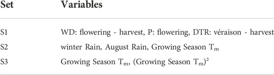
TABLE 4. Sets of predictors.

2.2.3 Linear regression models

Owing to the very nature of an agricultural yield prediction problem, where input-output couples can only be obtained once per harvest, the data at hand is sparse. This increases the risk of overfitting, namely the phenomenon by which a flexible model would adapt too much to the dataset variance and be unable of generalization (Hawkins, 2004). The Ordinary Least Squares model (Goldberger, 1962), noted OLS, has no hyperparameter and reduced flexibility, which reduces the probability of overfitting the training data. But its main advantage resides in the clear explanation that it gives of the relationships between predictor variables and the output: this is probably why this model is used in the overwhelming majority of econometric models in the literature (Jones and Davis, 2000; Esteves and Manso Orgaz, 2001; Jones and Storchmann, 2001; Jones et al., 2005; Haeger and Storchmann, 2006; Ashenfelter, 2008; Corsi and Ashenfelter, 2019).

2.2.4 Local least-squares kernel regression

The environment of a grapevine cultivar is described through the french word Terroir as the intricate relationship between climate, soil, and production methods (Seguin, 1986). For Bordeaux Grands crus, although the soils and cultivars remain mostly unchanged, deep evolutions are ongoing in both climate and production methods.

The 2.5°C increase in average growing season temperature in Bordeaux between 1960 and 2017 (illustrated for Saint-Emilion in Supplementary Appendix Figure S1), undoubtedly has significant effects on the plants, for instance causing phenological events to happen earlier (van Leeuwen and Darriet, 2016). On the side of the vine-growing methods, literature lists a myriad of innovations (see Gutiérrez-Gamboa et al., 2021 for a recent review), which seem to also have had a tangible effect, for instance by allowing the vineyard to maintain high fruit and wine quality until now (Gambetta and Kurtural, 2021) despite previous predictions of decline (Jones et al., 2005; Hannah et al., 2013).

Due to these long-term changes in the grapevine’s growing conditions, Almaraz (2015) evidenced that the impact of average growing season temperature on wine quality in Bordeaux has evolved over the last decades. We extrapolate this finding to hypothesize that other weather variables also have an evolving effect.

Then according to this hypothesis, in order to model the impact of certain weather parameters on wine quality, models with time-invariant effect cannot perform on long vintage series. Thus we want to find a model that can adapt its coefficients for a time-varying impact. However, the scarcity of the data at hand also raises the necessity of always keeping a memory of the oldest data points. Local Least Squares (LLS) kernel regression solves this dilemma, while still presenting the desirable properties of explainability and adversity to overfitting presented above. The goal of this method is to improve linear regression by applying more weight in the training to temporally close data points. This intuition is represented in Figure 5.

The problem of wine quality modeling is expressed as an extension of Equation 1 for several weather parameters. The logarithm of price of vintage $v,$ noted $y_v$, is estimated by the multivariate local linear estimator:

$y_v={\alpha }_v+{\displaystyle \sum }_{i\in [1,m]}{\beta }_{i,v} *x_{i,v}$

with ${\left\{{\beta }_{i,t}\right\}}_{i\in [1,m]}$ the coefficients associated with each parameter.

In the setting of LLS regression, we calculate the coefficients $\alpha$ and $\beta$ used in the prediction of vintage $v$ as the solution to the following optimization problem, which is simply a least-squares loss function, with the key difference that each term is attributed a different weight. This weight is determined by a kernel function K that decreases with the distance $v–t$ between the predicted vintage $v$ and the training data point of vintage $t$, and this distance is rescaled by a bandwidth parameter $h$:

$\widehat{{\alpha }_{K,h,v}},{\widehat{\left\{{\beta }_{K,h,v}\right\}}}_{i\in [1,m]}=\underset{\alpha \in {\mathbb{R}}^n,\beta \in {\mathbb{R}}^{n*m}}{\mathrm{a}\mathrm{r}\mathrm{g}\mathrm{m}\mathrm{i}\mathrm{n}}{\displaystyle \sum }_t{\left(y_t-{\alpha }_t-{\displaystyle \sum }_{i\in [1,m]}{\beta }_{i,t}*x_{i,t}\right)}^2*K\left(\frac{v-t}{h}\right)$

To solve this equation, we write it in matricial form, with the intercept $\widehat{{\alpha }_{K,h,v}}$ and coefficients $\widehat{{\beta }_{K,h,v}}$ integrated into a single matrix $\widehat{{\beta }_{K,h,v}}$:

$\widehat{{\beta }_{K,h,v}}={\underset{\beta }{\mathrm{a}\mathrm{r}\mathrm{g}\mathrm{m}\mathrm{i}\mathrm{n}}\left(Y_v-\beta X_v\right)}^T{W}_{K,h,v}\left(Y_v-\beta X_v\right)$

With $Y_v$ the column matrix containing all training prices, the matrix of weather parameters $\mathrm{X}=\left[\begin{array}{cccc}1& x_{1, t_{\mathit{min}}}& \cdots & x_{m, t_{\mathit{min}}}\\ ⋮& ⋮& \ddots & ⋮\\ 1& x_{1, t_{\mathit{max}}}& \cdots & x_{m, t_{\mathit{max}}}\end{array}\right]$, the coefficient matrix $\beta =\left[\begin{array}{cccc}{\alpha }_{v_{\mathit{min}}}& {\beta }_{1, t_{\mathit{min}}}& \cdots & {\beta }_{m, t_{\mathit{min}}}\\ ⋮& ⋮& \ddots & ⋮\\ {\alpha }_{v_{\mathit{max}}}& {\beta }_{1, t_{\mathit{max}}}& \cdots & {\beta }_{m, t_{\mathit{max}}}\end{array}\right]$ , and $W_{K,h,v}$ the diagonal matrix of weights $\mathrm{d}\mathrm{i}\mathrm{a}\mathrm{g}\left(\mathrm{K}\left(\frac{v-t_{\mathit{min}}}{h}\right), \mathrm{K}\left(\frac{v-\left(t_{\mathit{min}}+1\right)}{h}\right),\dots , \mathrm{K}\left(\frac{v-t_{\mathit{max}}}{h}\right)\right)$.

Ruppert et al. (1995) give the closed-form solution to this optimization problem:

${\beta }_{K,h,v}={\left(X_v^T{W}_{K,h,v}{X}_v\right)}^{-1}{X}_v^T{W}_{K,h,v}{Y}_v$

Which in turn yields the estimated price:

$f_{K,h,v}={{\beta }_{K,h,v}{X}_v=\left(X_v^T{W}_{K,h,v}{X}_v\right)}^{-1}{X}_v^T{W}_{K,h,v}{Y}_v{X}_v$

Note that in the above equation, $W_{K,h,v}$ depends on a scalar bandwidth parameter $h$, which must be chosen depending on the data available—and in our setting, the prediction of each vintage $v$ has access to data up to vintage $v-1$. We follow the cross-validation criterion, introduced by Clark (1977), which outperforms competitors in the case of multivariate prediction on small datasets (Köhler et al., 2014) as is the case here. Thus, the bandwidth $h_{K,v}$ for prediction of vintage v with kernel function K is set as the minimiser of the leave-out square error:

$h_{K,v}=\underset{h\in \mathbb{R}}{\mathrm{a}\mathrm{r}\mathrm{g}\mathrm{m}\mathrm{i}\mathrm{n}}{\displaystyle \sum }_t{\left({\beta }_{K,h,t,-t}{X}_t-y_t\right)}^2$

With ${\beta }_{K,h,t,-t}$ the leave-out estimator for year $t$, calculated from all available years except year $t$ to prevent overfitting.

2.2.5 Baseline: Widely used machine learning models

Widely used machine learning models have also been implemented to represent a panel of commonly used methods as a baseline against which to compare the OLS and LLS predictions. A simple Decision Tree (Quinlan, 1986), Random Forest (Breiman, 2001), Gradient Boosting (Friedman, 2001), and Single Value Regressor (Vapnik, 1995). All these implementations use the Python Scikit-learn package (Pedregosa et al., 2011). These models have been selected because they can provide decent performance on small datasets (here, the worst case is the prediction of vintage 1994, where training uses the 34 vintages from 1960 to 1993). But none of these models have been used yet -to our knowledge-in an academic study on grape price or yield prediction, and we do not expect them to yield good performance.

3 Results

The models are trained and tested on each of the vineyards mentioned in part 2.1.2 Long-term wine prices. The median value across all vineyards for the three metrics discussed in part 2.3.1 are displayed in Table 5. For the sake of clarity, only the versions of models trained on the S1 set of variables (see) are displayed for most models, as they yield the best performance.

TABLE 5

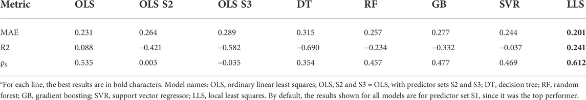
TABLE 5. Compared model scores, 1994–2013 timeframe.

Comparing the relative performance of different predictor sets on the same models proves that tailoring the model to the phenology of the grapevine helps achieve good predictive accuracy: for the OLS model, the S1 set of variables, aggregated along the phenological stages of the grapevine, outperforms by large the classical sets S2 and S3 (Welch t-test: p-value < 0,05 on all three metrics).

For all three metrics, LLS outperforms all other models, and the performance difference with the second runner-up, the OLS model, is significant (Welch t-test: p-value < 0.05 on all three metrics). Embedding the time-variation of coefficients into the architecture of the model gives it a strong advantage over fixed-coefficient models.

Figures 6A, B compare predictions and real prices for one of the vineyards, Château Calon-Ségur. The price comparison of Figure 6A, representative of the model behaviour on several other vineyards not displayed here, shows that although the model efficiently captures most of the price variations, it has more difficulty predicting some of the highest prices. This could be an indication that for some of the top vintages, prices can go far higher than their quality alone would indicate.

FIGURE 6

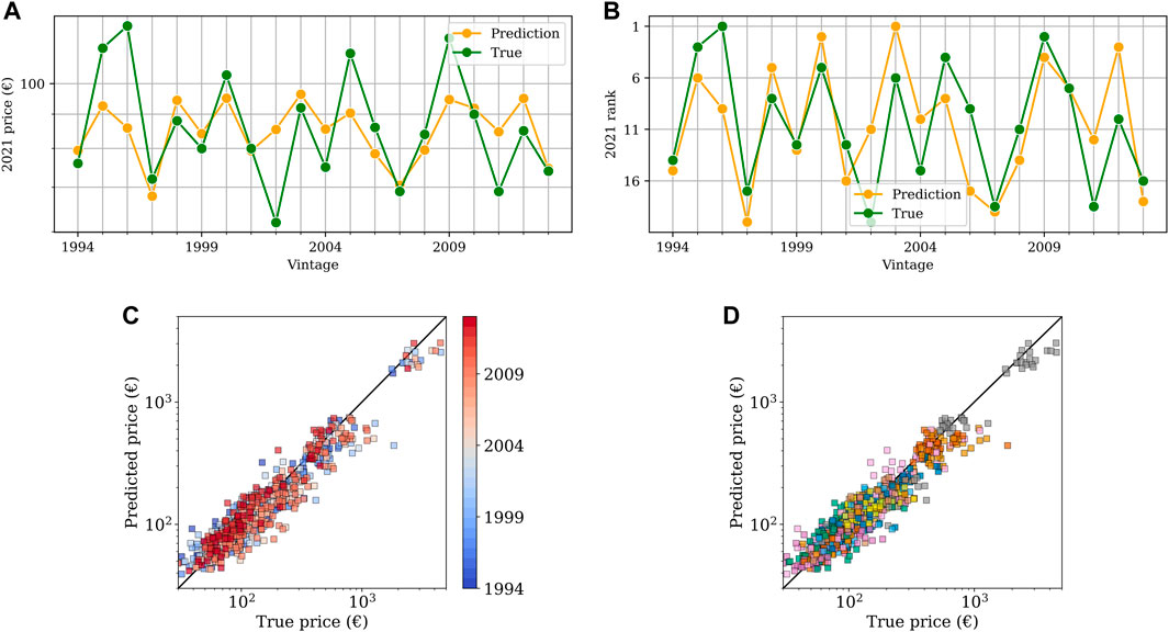
FIGURE 6. (A) Compared LLS model predicted and true price, vineyard Château Calon-Ségur (B) Compared LLS model predicted and true rank, vineyard Château Calon-Ségur. Compared predicted and true prices for the LLS model, all vineyards, colored by vintage (C) and vineyard (D).

Figure 6 shows the fit between true and predicted prices. As we can observe on the left chart, the fit seems to be better in recent years, which we could attribute to the training set using a longer time series of data.

The best-performing LLS kernel regression model has also been compared to the primeur grades of critic Robert Parker on the timeframe 1994 to 2013 when they were available. The grades are written on a scale of 0–100, and the relationship of this scale with quality is hard to linearly quantify. Therefore, following the example of Cyr et al. (2019), we use the Spearman rank correlation: how well do predicted prices on one side, and ratings on the other, rank compared to real prices. For a selected set of individual vineyards, Robert Parker’s ratings have a median score of 0.630, while the LLS model beats them with a higher median score of 0.678 (see Supplementary Appendix Table S2).

4 Discussion

4.1 Outcomes and discoveries

Upon comparing the relative performance of different models (Table 5), two components are observed to improve the predictive accuracy of the model. The first improvement, evidenced by the better performance of the phenology-adapted S1 set of variables compared to the calendar-based S2 and S3 (see Table 4 for a description of the variables used in each set), is the usage of phenology-adapted features, as introduced by Jones and Davis (2000). The necessity of using phenology-adapted features stems from the different needs of the grapevine across different periods of its lifecycle. For instance, the ultimate impact of temperature stress on yield or reproductive fitness depends on the developmental stage at which it occurs (Hatfield and Prueger, 2015; Gray and Brady, 2016). Distinguishing between these different lifecycle periods allows for capturing the changing needs of the grapevine. The weather predictors with the strongest positive impact on prices are the water deficit between flowering and harvest and the diurnal temperature range during the ripening phase (véraison to harvest). The parameter with the strongest negative impact was the precipitation during flowering; to our knowledge, it is the first time in an academic study that flowering precipitation is identified as a significant negative factor.

The second improvement of the model’s predictive accuracy was brought about by using a time-varying model. It is proven by Almaraz (2015) that the positive impact of a higher-than-average growing season temperature had progressively been waning over the last decades. This author postulates that this time variation in the impact of weather variables on wine quality is due partly to climate change, and partly to the adaptation of production methods. As a result of this variation, properly embedding time variation into a predictive model should improve its performance. We confirm this hypothesis by using the LLS regression model, which provides better performance than fixed-coefficient models.

The predictive model using these two features achieves state-of-the-art performance in the Bordeaux region for the prediction of wine prices, by even beating the predictive accuracy of early primeur grades from world-renowned Robert Parker, with the additional advantage of being available earlier i.e., directly after the harvest rather than next April. By proving that publicly available weather parameters can be combined to perform better prediction than the critic who had a defining impact on the Bordeaux vineyard, with the additional advantage of being available earlier, this study opens the way for the usage of quantitative models in premium wine price determination.

4.2 Limitations

This study was constrained by the hypothesis of ex-ante testing, where we wanted to reproduce the real use case of a price prediction model. For the prediction of vintage $v$, the predictive model was trained with the 2021 prices of vintages up to $v$ - 1. But this is not completely representative of the real setting, where training cannot use long-term price data for recent vintages, because it is not available yet: this gives an edge to the predictive model. It is also important to keep in mind that Robert Parker’s critical grade, originally given as a lower and upper bound, was averaged in this study into a unique grade so as to obtain a single quality prediction. This removes some of the information he expressed but does not distort his general prediction of quality, which is still beaten by the predictive model. And anyway, the correlation between critical grades and prices is strongly artificially increased by the auto-fulfilling prophecy character of the primeur ratings mentioned in the literature (Ali et al., 2008) and evidenced in Part 2.1.5.

4.3 Directions for future research

This study opens ways for further research. Knowledge of the impact of weather features on quality could be refined by contrasting different cultivars or soils, although gathering granular phenology data is difficult. Extension to other regions, wherever the necessary historical records of the phenological calendar can be obtained, would allow comparing the variation of the impact of different weather parameters, along with the different stages of warming experienced in the region.

Owing to the changing needs of the grapevine throughout its cycle, this study drew on teachings from previous papers to design features aggregated according to the phenological calendar of the grapevine. These features yield a better predictive result than features aggregated over a yearly-invariant timeframe. As many crops similarly undergo very contrasted phenological phases, the principle of using phenology-adapted features could have interesting generalizations.

The outperforming of critical ratings and other models by LLS regression brings a novel contribution to the field of agricultural systems modeling. Due to systematic changes in both climate and production methods, many weather parameters have a varying impact on grape quality over time: as a result, including a time-varying component in the modeling of this agricultural system improved predictive performance. This novel introduction of a time-varying model could yield insightful results when applied to other wine regions similarly undergoing strong adaptation to climate change, such as Napa Valley (California, United States) or New South Wales (Australia).

Data availability statement

The datasets presented in this study can be found in online repositories. The names of the repository/repositories and accession number(s) can be found in the article/Supplementary Material.

Author contributions

AR, LA, and FT contributed to conception and design of the study. AR performed the data collection and treatment as well as the statistical analysis and design of the predictive model. AR wrote the first draft of the manuscript. AR, LA and FT wrote sections of the manuscript. All authors contributed to manuscript revision, read, and approved the submitted version.

Funding

This study was funded by the Open access grand of the University of Cambridge.

Acknowledgments

The authors are specially grateful towards the staff of Château Latour for their support of the project. They would also like to thank the French meteorological agency Météo-France for providing the necessary weather data, as well as the online wine merchant IDealwine for their auction prices data. Two reviewers should also be thanked for their insightful comments.

Conflict of interest

The authors declare that the research was conducted in the absence of any commercial or financial relationships that could be construed as a potential conflict of interest.

Publisher’s note

All claims expressed in this article are solely those of the authors and do not necessarily represent those of their affiliated organizations, or those of the publisher, the editors and the reviewers. Any product that may be evaluated in this article, or claim that may be made by its manufacturer, is not guaranteed or endorsed by the publisher.

Supplementary material

The Supplementary Material for this article can be found online at: https://www.frontiersin.org/articles/10.3389/fenvs.2022.1020867/full#supplementary-material

Footnotes

¹https://www.idealwine.com/, personal communication.

References

Alem, H., Rigou, P., Schneider, R., Ojeda, H., and Torregrosa, L. (2019). Impact of agronomic practices on grape aroma composition: A review. J. Sci. Food Agric. 99 (3), 975–985. doi:10.1002/jsfa.9327

PubMed Abstract | CrossRef Full Text | Google Scholar

Ali, H. H., Lecocq, S., and Visser, M. (2008). The impact of Gurus: Parker grades and en primeur wine prices. Econ. J. 118 (529), F158–F173. doi:10.1111/j.1468-0297.2008.02147.x

CrossRef Full Text | Google Scholar

Almaraz, P. (2015). Bordeaux wine quality and climate fluctuations during the last century: Changing temperatures and changing industry. Clim. Res. 64 (3), 187–199. doi:10.3354/cr01314

CrossRef Full Text | Google Scholar

Aristodemou, L., and Tietze, F. (2018). The state-of-the-art on intellectual property analytics (IPA): A literature review on artificial intelligence, machine learning and deep learning methods for analysing intellectual property (IP) data. World Pat. Inf. 55, 37–51. doi:10.1016/j.wpi.2018.07.002

CrossRef Full Text | Google Scholar

Ashenfelter, O. (2008). Predicting the quality and prices of Bordeaux wine. Econ. J. 118 (529), F174–F184. doi:10.1111/j.1468-0297.2008.02148.x

CrossRef Full Text | Google Scholar

Baciocco, K. A., Davis, R. E., and Jones, G. V. (2014). Climate and Bordeaux wine quality: Identifying the key factors that differentiate vintages based on consensus rankings. J. Wine Res. 25 (2), 75–90. doi:10.1080/09571264.2014.888649

CrossRef Full Text | Google Scholar

Biss, A., and Ellis, R. (2021). Modelling Chablis vintage quality in response to inter-annual variation in weather. OENO One 55 (3), 209–228. Article 3. doi:10.20870/oeno-one.2021.55.3.4709

CrossRef Full Text | Google Scholar

Blank, M., Hofmann, M., and Stoll, M. (2019). Seasonal differences in Vitis vinifera L. Cv. Pinot noir fruit and wine quality in relation to climate. OENO One 53 (2), 189–203. doi:10.20870/oeno-one.2019.53.2.2427

CrossRef Full Text | Google Scholar

Breiman, L. (2001). Random forests. Mach. Learn. 45 (1), 5–32. doi:10.1023/A:1010933404324

CrossRef Full Text | Google Scholar

Byron, R. P., and Ashenfelter, O. (1995). Predicting the quality of an unborn grange. Econ. Rec. 71 (1), 40–53. doi:10.1111/j.1475-4932.1995.tb01870.x

CrossRef Full Text | Google Scholar

Castellarin, S. D., Matthews, M. A., Di Gaspero, G., and Gambetta, G. A. (2007). Water deficits accelerate ripening and induce changes in gene expression regulating flavonoid biosynthesis in grape berries. Planta 227 (1), 101–112. doi:10.1007/s00425-007-0598-8

PubMed Abstract | CrossRef Full Text | Google Scholar

Chicco, D., Warrens, M. J., and Jurman, G. (2021). The coefficient of determination R-squared is more informative than SMAPE, MAE, MAPE, MSE and RMSE in regression analysis evaluation. PeerJ Comput. Sci. 7, e623. doi:10.7717/peerj-cs.623

PubMed Abstract | CrossRef Full Text | Google Scholar

Clark, R. M. (1977). Non-parametric estimation of a smooth regression function. J. R. Stat. Soc. Ser. B Methodol. 39 (1), 107–113. doi:10.1111/j.2517-6161.1977.tb01611.x

CrossRef Full Text | Google Scholar

Corsi, A., and Ashenfelter, O. (2019). Predicting Italian wine quality from weather data and expert ratings. J. Wine Econ. 14 (3), 234–251. doi:10.1017/jwe.2019.41

CrossRef Full Text | Google Scholar

Cyr, D., Kwong, L., and Sun, L. (2019). Who Will Replace Parker? A Copula Function Analysis of Bordeaux en Primeur Wine Raters. J. Wine Econ. 14 (2), 133–144. doi:10.1017/jwe.2019.4

CrossRef Full Text | Google Scholar

de Rességuier, L., Mary, S., Le Roux, R., Petitjean, T., Quénol, H., and van Leeuwen, C. (2020). Temperature variability at local scale in the Bordeaux area. Relations with environmental factors and impact on vine phenology. Front. Plant Sci. 11, 515. doi:10.3389/fpls.2020.00515

PubMed Abstract | CrossRef Full Text | Google Scholar

Duteau, J., Guilloux-Benatier, M., and Seguin, G. (1981). Influence des facteurs naturels sur la maturation du raisin, en 1979, à Pomerol et Saint-Emilion. OENO One 15 (1), 1–27. doi:10.20870/oeno-one.1981.15.1.1358

CrossRef Full Text | Google Scholar

Esteves, M. A., and Manso Orgaz, M. D. (2001). The influence of climatic variability on the quality of wine. Int. J. Biometeorology 45 (1), 13–21. doi:10.1007/s004840000075

PubMed Abstract | CrossRef Full Text | Google Scholar

Fayolle, E., Follain, S., Marchal, P., Chéry, P., and Colin, F. (2019). Identification of environmental factors controlling wine quality: A case study in Saint-Emilion Grand Cru appellation, France,. Science of the Total Environment. 694 133718 doi:10.1016/j.scitotenv.2019.133718

PubMed Abstract | CrossRef Full Text | Google Scholar

Fraga, H., Malheiro, A. C., Moutinho-Pereira, J., and Santos, J. A. (2013). Future scenarios for viticultural zoning in Europe: Ensemble projections and uncertainties. Int. J. Biometeorol. 57 (6), 909–925. doi:10.1007/s00484-012-0617-8

PubMed Abstract | CrossRef Full Text | Google Scholar

Friedman, J. H. (2001). Greedy function approximation: A gradient boosting machine. Ann. Stat. 29 (5), 1189–1232. doi:10.1214/aos/1013203451

CrossRef Full Text | Google Scholar

Gambetta, G. A., and Kurtural, S. K. (2021). Global warming and wine quality: Are we close to the tipping point? OENO One 55 (3), 353–361. doi:10.20870/oeno-one.2021.55.3.4774

CrossRef Full Text | Google Scholar

Goldberger, A. S. (1962). Best linear unbiased prediction in the generalized linear regression model. J. Am. Stat. Assoc. 57 (298), 369–375. doi:10.1080/01621459.1962.10480665

CrossRef Full Text | Google Scholar

Gray, S. B., and Brady, S. M. (2016). Plant developmental responses to climate change. Dev. Biol. 419 (1), 64–77. doi:10.1016/j.ydbio.2016.07.023

PubMed Abstract | CrossRef Full Text | Google Scholar

Gutiérrez-Gamboa, G., Zheng, W., and Martínez de Toda, F. (2021). Current viticultural techniques to mitigate the effects of global warming on grape and wine quality: A comprehensive review. Food Res. Int. 139, 109946. doi:10.1016/j.foodres.2020.109946

PubMed Abstract | CrossRef Full Text | Google Scholar

Haeger, J. W., and Storchmann, K. (2006). Prices of American pinot noir wines: Climate, craftsmanship, critics. Agric. Econ. 35 (1), 67–78. doi:10.1111/j.1574-0862.2006.00140.x

CrossRef Full Text | Google Scholar

Hannah, L., Roehrdanz, P. R., Ikegami, M., Shepard, A. V., Shaw, M. R., Tabor, G., et al. (2013). Climate change, wine, and conservation. Proc. Natl. Acad. Sci. U. S. A. 110 (17), 6907–6912. doi:10.1073/pnas.1210127110

PubMed Abstract | CrossRef Full Text | Google Scholar

Hatfield, J. L., and Prueger, J. H. (2015). Temperature extremes: Effect on plant growth and development. Weather Clim. Extrem. 10, 4–10. doi:10.1016/j.wace.2015.08.001

CrossRef Full Text | Google Scholar

Hawkins, D. M. (2004). The problem of overfitting. J. Chem. Inf. Comput. Sci. 44 (1), 1–12. doi:10.1021/ci0342472

PubMed Abstract | CrossRef Full Text | Google Scholar

Jones, G. V., and Davis, R. E. (2000). Climate influences on grapevine phenology, grape composition, and wine production and quality for Bordeaux, France. Am. J. Enology Vitic. 51 (3), 249–261. Scopus.

Google Scholar

Jones, G. V., and Storchmann, K.-H. (2001). Wine market prices and investment under uncertainty: An econometric model for Bordeaux Crus Classés. Agric. Econ. 26 (2), 115–133. doi:10.1016/S0169-5150(00)00102-X

CrossRef Full Text | Google Scholar

Jones, G. V., White, M. A., Cooper, O. R., and Storchmann, K. (2005). Climate change and global wine quality. Clim. Change 73 (3), 319–343. doi:10.1007/s10584-005-4704-2

CrossRef Full Text | Google Scholar

Köhler, M., Schindler, A., and Sperlich, S. (2014). A review and comparison of bandwidth selection methods for kernel regression. Int. Stat. Rev. 82 (2), 243–274. doi:10.1111/insr.12039

CrossRef Full Text | Google Scholar

Lancashire, P. D., Bleiholder, H., Boom, T. V D, Langeluddeke, P., Stauss, R., Weber, E., et al. (1991). A uniform decimal code for growth stages of crops and weeds. Ann. Appl. Biol. 119 (3), 561–601. doi:10.1111/j.1744-7348.1991.tb04895.x

CrossRef Full Text | Google Scholar

Matthews, M. A., and Anderson, M. M. (1988). Fruit ripening in Vitis vinifera L.: Responses to seasonal water deficits. Am. J. Enology Vitic. 39 (4), 313–320.

Google Scholar

Oczkowski, E. (1994). A hedonic price function for Australian premium table wine. Aust. J. Agric. Econ. 38 (1), 93–110. doi:10.1111/j.1467-8489.1994.tb00721.x

CrossRef Full Text | Google Scholar

Oczkowski, E., and Doucouliagos, H. (2015). Wine prices and quality ratings: A meta-regression analysis. Am. J. Agric. Econ. 97 (1), 103–121. doi:10.1093/ajae/aau057

CrossRef Full Text | Google Scholar

Pedregosa, F., Varoquaux, G., Gramfort, A., Michel, V., Thirion, B., Grisel, O., et al. (2011). Scikit-learn: Machine learning in Python. J. Mach. Learn. Res. 12, 2825–2830. Scopus.

Google Scholar

Pérez-Magariño, S., and González-San José, M. L. (2006). Polyphenols and colour variability of red wines made from grapes harvested at different ripeness grade. Food Chem. 96 (2), 197–208. doi:10.1016/j.foodchem.2005.02.021

CrossRef Full Text | Google Scholar

Quinlan, J. R. (1986). Induction of decision trees. Mach. Learn. 1 (1), 81–106. doi:10.1023/A:1022643204877

CrossRef Full Text | Google Scholar

Riou, C., Pieri, P., and Clech, B. L. (1994). Consommation d’eau de la vigne en conditions hydriques non limitantes. Formulation simplifiée de la transpiration. Vitis 33, 109.

Google Scholar

Roberts, P. W., and Reagans, R. (2007). Critical exposure and price-quality relationships for New world wines in the U.S. Market. J. Wine Econ. 2 (1), 84–97. doi:10.1017/S1931436100000316

CrossRef Full Text | Google Scholar

Ruppert, D., Sheather, S. J., and Wand, M. P. (1995). An effective bandwidth selector for local least squares regression. J. Am. Stat. Assoc. 90 (432), 1257–1270. doi:10.1080/01621459.1995.10476630

CrossRef Full Text | Google Scholar

Schamel, G., and Anderson, K. (2003). Wine quality and varietal, regional and winery reputations: Hedonic prices for Australia and New Zealand. Econ. Rec. 79 (246), 357–369. doi:10.1111/1475-4932.00109

CrossRef Full Text | Google Scholar

Seguin, G. (1986). ‘Terroirs’ and pedology of wine growing. Experientia 42 (8), 861–873. doi:10.1007/BF01941763

CrossRef Full Text | Google Scholar

Storchmann, K. (2012). Wine economics. J. Wine Econ. 7 (1), 1–33. Article 1. doi:10.1017/jwe.2012.8

CrossRef Full Text | Google Scholar

Tonietto, J., and Carbonneau, A. (2004). A multicriteria climatic classification system for grape-growing regions worldwide. Agric. For. Meteorology 124 (1), 81–97. doi:10.1016/j.agrformet.2003.06.001

CrossRef Full Text | Google Scholar

van Leeuwen, C., and Darriet, P. (2016). The impact of climate change on viticulture and wine quality. J. Wine Econ. 11 (1), 150–167. doi:10.1017/jwe.2015.21

CrossRef Full Text | Google Scholar

van Leeuwen, C., Friant, P., Choné, X., Tregoat, O., Koundouras, S., and Dubourdieu, D. (2004). Influence of climate, soil, and cultivar on terroir. Am. J. Enology Vitic. 55 (3), 207–217. Scopus.

Google Scholar

van Leeuwen, C., Trégoat, O., Choné, X., Bois, B., Pernet, D., and Gaudillère, J.-P. (2009). Vine water status is a key factor in grape ripening and vintage quality for red Bordeaux wine. How can it be assessed for vineyard management purposes? OENO One 43 (3), 121–134. doi:10.20870/oeno-one.2009.43.3.798

CrossRef Full Text | Google Scholar

Vapnik, V. N. (1995). “Constructing learning algorithms,” in The nature of statistical learning theory. Editor V. N. Vapnik (Springer), Heidelberg, Germany 119–166. doi:10.1007/978-1-4757-2440-0_6

CrossRef Full Text | Google Scholar

Vidal, J.-P., Martin, E., Franchistéguy, L., Baillon, M., and Soubeyroux, J.-M. (2010). A 50-year high-resolution atmospheric reanalysis over France with the Safran system. Int. J. Climatol. 30 (11), 1627–1644. doi:10.1002/joc.2003

CrossRef Full Text | Google Scholar

Zsófi, Z. S., Tóth, E., Rusjan, D., and Bálo, B. (2011). Terroir aspects of grape quality in a cool climate wine region: Relationship between water deficit, vegetative growth and berry sugar concentration. Sci. Hortic. 127 (4), 494–499. doi:10.1016/j.scienta.2010.11.014

CrossRef Full Text | Google Scholar