Improvement of a land fragmentation measurement model based on natural surface elements and road network

Land fragmentation is one of the most important factors hindering the mechanization and scale of agriculture. To further alleviate the negative impact of arable land fragmentation, a more accurate model for measuring arable land fragmentation is needed. Using 0.1 resolution UAV images and farm survey data, we obtained spatial and tenure data of farming land in Baidu Village through ArcGis and other software, and analyzed the results and correlations of farming plot area, plot shape and plot dispersion indicators in the study area. A road accessibility index that integrates terrain slope and road network is proposed to characterize the dispersion of land parcels for the first time, and is compared with two road accessibility models that do not take into account terrain slope and road network. The results show that the dispersion index of farm plots is the most influential indicator on the fragmentation of farm plots, followed by the area index of farm plots, and finally the shape index of farm plots; the new model of measuring the fragmentation of farm plots based on natural surface elements and road networks is closer to the real situation and more accurate in portraying the degree of fragmentation of farm plots.

Introduction

With the advancement of economic globalization, the process of world urbanization is accelerating. Currently, about 54% of the world’s population lives in urban areas, and this proportion is expected to reach 66% by 2050 (UNDESA, 2014; Masini et al., 2018). The large-scale transfer of agricultural labor to nonagricultural industries increases the opportunity cost of agricultural labor (Kawasaki, 2011). The United Nations predicts that by 2050, the world population is expected to reach 9.3 billion, and the global population will reach 10.1 billion in 2100 (United Nations Population Division, 2011). The continuously growing population, limited arable land resources, and dwindling agricultural population have placed enormous pressure on world food security (Nair, 2014). To provide a maximum guarantee to meet the growing food demand of mankind, it is necessary to improve the intensive utilization of cultivated land. The ability to achieve a certain scale benefit has become the key to promoting agricultural development and ensuring food security. Land fragmentation (LF) is a prominent feature of cropland use in agricultural production in developing countries, and the supply of cropland for food production is increasingly limited (Niroula and Thapa, 2007; Di Falco et al., 2010). Under the influence of many factors, such as natural environment and social economy, LF in China is serious problem (Tan et al., 2006). LF refers to the phenomenon that a farmer’s land resources are scattered and not concentrated (Latruffe and Piet, 2014; Lu et al., 2018). Related studies have focused on the basic plots of farming operations, exploring the essential attributes of the plots and studying the causes of LF (Janus et al., 2016). Also, basic characteristics of LF are included, including the distribution of plots cultivated by farmers, their proximity to households (Niroula and Thapa, 2005), the size of plots cultivated (Lu et al., 2018), the number of plots (Wan and Cheng, 2001), and plot shape (Demetriou et al., 2013).

LF is a pattern of arable land resource utilization that is contrary to the scale of arable land management. This pattern enriches the diversity of agricultural production in China and reduces the risk of agricultural cultivation (Nguyen et al., 1996; Van Hung et al., 2007; Tan et al., 2021). However, there are certain negative effects, and affects the efficient use of land resources and national food security. Disorganized, interspersed, and scattered plot distribution is an important aspect of cultivated plot distribution in China (Qi and Dang, 2018). This distribution can increase commuting costs (Latruffe and Piet, 2014; Wang and Wang, 2010). When the number of plots owned by farmers is large and scattered, the cost of transportation and traveling time from the homestead to each plot will increase (de Garis De Lisle, 2010; del Corral et al., 2011; Niroula and Thapa, 2005). Farmers’ traveling time will increase under the influence of terrain slope and distance traveled, which not only causes invariance to material transportation and plot irrigation management but also increases labor input, thus reducing farmers’ economic returns (Niroula and Thapa, 2007; Kawasaki, 2010). Considering these conditions, farmers will pay less attention to remote and low-quality plots, and this type of plot often has much higher input costs than net benefits, and farmers will abandon these plots (Carter and Yao, 2002; de Garis De Lisle, 2010; Lu et al., 2018). In addition, LF has a hindering effect on agricultural mechanization and productivity (Blarel et al., 1992; Wan and Cheng, 2001; Ali and Deininger, 2015). In the case of growing maize, late rice, and wheat, the production efficiency decreases by 4%, 15%, and 17% when the degree of cultivated land fineness increases by one unit, respectively (Wan and Cheng, 2001). With the small size of arable plots, farmers need to invest in more labor to increase production value (Lu et al., 2018), and the increase in the number of plots increases the amount of labor invested by farmers. In addition, when plots are small and irregularly shaped, farmers often will not develop advanced agricultural technologies and may even abandon this land (Van Hung et al., 2007; Gónzalez et al., 2007), which further limits productivity and hinders agricultural modernization.

To mitigate these negative impacts of LF, the Chinese government conducts policy control, and to fully manage the impacts of LF, policy-makers and planners need scientific indicators to measure the extent of LF (Igozurike, 1974; Januszewski, 1968; Simmons, 1964). Based on the definition of land fractionation above, we know that the plot dispersion, plot size, and plot shape indicators ideally should be incorporated into a comprehensive measurement model to accurately measure the degree of LF. Currently there are more accepted ways of evaluating parcel size and parcel shape, among these indicators, plot area uses the Simpson index to combine the number of plots and plot area, which accurately reflects the area characteristics of plots. The plot shape index uses the standard squares and circles as standard measure, which reflects the shape characteristics of the plot to a certain extent. However, there are no accurate indicators for the dispersion of plots in the academic community, the current indicators characterizing the dispersion of farmers’ plots include distances, such as the distance from farmers’ homesteads to each of their plots as well as the distance between plots. These distances are Euclidean distances or road network distances. Other studies have used farmer’s commuting time to reflect the fragmentation of plots (Ge and Zhao, 2019). And calculating the shortest cumulative time from farmers’ homesteads to each of their plots through iteration, which is the road accessibility of farmers. It uses commuting time to combine two factors, namely distance and walking speed, to more comprehensively and accurately reflect the dispersion of parcels. Road accessibility refers to the ease of getting from the starting point to the end point (Páez et al., 2012), the two main factors in measuring road accessibility index are walking speed or distance (Hess and Almeida, 2007; Higgins, 2019). Some studies have used Euclidean distance, which ignores the distance of the road networks formed by complex topographic environments (Zhao, 2011; Ge and Zhao, 2019). Alternatively, walking speed was set to the normal human walking speed (5 km/h) and was a constant value (Ge and Zhao, 2019), which was determined under the assumption of a flat walking plane and a constant walking speed of 5 km/h. Although this planar approach is not problematic in a two-dimensional and topographically flat study area, this approach can overestimate (or underestimate) walkability in a topographically diverse environment (Higgins, 2019). Because walking speed and terrain are not constant, in addition to personal ability, time pressure, and other factors, walking speed varies with the slope of the walking environment (Lee et al., 2015; Aghabayk et al., 2021). Figure 1 shows the terrain affects the road accessibility, and road accessibility is much lower in areas with more undulating terrain (Figure 1A) than in areas with flat terrain (Figure 1B). This is especially true in mountainous areas, where the terrain is undulating and the surface is rugged and broken. The slope of the pedestrian road has a significant impact on the walking speed of farmers, thus affecting the commuting costs of farmers from their homesteads to their plots. Therefore, use of the LF measurement model without considering the terrain factor is not suitable for mountainous areas.

FIGURE 1

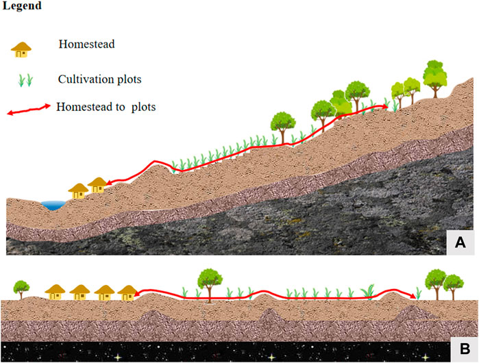
FIGURE 1. Schematic diagram of the distribution of homesteads and plots. Figure 1A shows that the road network is affected by the topography in the mountainous areas. Figure 1B shows the road network in a flat terrain.

To address the shortcomings of the LF measurement model, and based on the previous research, we integrated the topographic slope into the measurement model and integrated natural surface elements and road networks to build an LF measurement model that is more realistic and applicable to plain or mountainous areas. We accurately portrayed the degree of fragmentation of cultivated land and provided a basic reference for academic research and policy formulation.

Materials and methods

General situation of the research area

The existing measurement model is applicable to the plain areas, which are less spatially heterogeneous. To consider the extent to which the fine fragmentation of mountainous cultivated land is affected by topography, we selected a typical mountainous cultivated area. Baidu Village, Jianhe County, Qiandongnan Prefecture, Guizhou Province, is a typical mountainous village (108°47′9 ″E–108°47′30 ″E, 26°4011 ″N–26°40′23 ″N) (Figure 2) located on the banks of the Qingshui River. It is 30 km from Nanzhai Town and has two natural villages: the Upper Baidu Village and Lower Baidu Village. Under the jurisdiction of 27 village groups, the village is dominated by the Miao ethnic group. In 2020, the total resident population had reached 1,655. The economy of Baidu Village is mainly agricultural. The village land area is 1241.216 hm², the total arable land area is 113.407 hm², the average arable land area is 0.067 hm², the forestland area is 186.667 hm², and the per capita forestland area is 0.112 hm². It is a typical example of the fragmentation of arable land in mountainous areas.

FIGURE 2

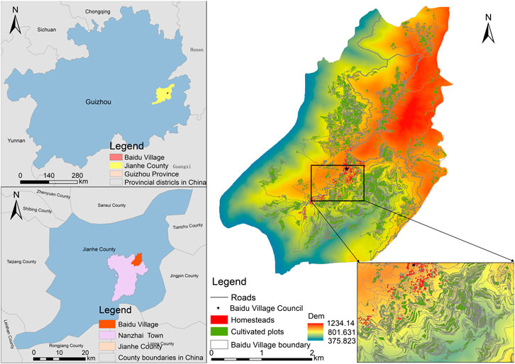
FIGURE 2. The study area.

Research method

Village and farmer model construction

Rural farmland in China is generally dominated by farm households’ contracting and management, and is also affected by village contracting rights, land adjustment, and intra-village transfer, which affect LF to some extent. For this reason, we constructed LF models for farming land at the farm household and village levels, respectively.

The main structure of the farm households model is as follows: we selected the attribute indicators characterizing the fine fragmentation of farming land for inclusion in the model, calculated the values of each characterizing attribute indicator, and summed the values of each characterizing attribute indicator to obtain the farmer’s land fragmentation index (FLFI), according to the following equation:

$\mathbf{F}\mathbf{L}\mathbf{F}\mathbf{I}={\displaystyle \sum }_{\mathbf{i}=\mathbf{1}}^{\mathbf{n}}{\mathbf{F}}_{\mathbf{i}}(1)$

where Fi represents each indicator of cultivated land fine fragmentation; and n is the number of selected indicators. The range of FLFI is (0, 3), and the larger the value is, the higher the degree of fragmentation of farmers’ cultivated land.

The village model is calculated based on the cultivated FLFI of each farming household. The village farmland fragmentation index (VLFI) is the average value of each farming household’s FLFI. The formula is as follows:

$\mathbf{V}\mathbf{L}\mathbf{F}\mathbf{I}=\frac{{\displaystyle \sum }_{\mathbf{j}=\mathbf{1}}^{\mathbf{m}}{\mathbf{F}\mathbf{L}\mathbf{F}\mathbf{I}}_{\mathbf{j}}}{\mathbf{m}}(2)$

where FLFI_j is the cultivated land fragmentation index of farming household j; and m is the number of farming households in the village. The range of values of VLFI is (0, 3), and the larger the value is, the higher the degree of cultivated land fragmentation in the village.

Selection of evaluation indicators

The connotation of LF is reflected in the following four aspects: fragmented distribution of arable land plots operated by farmers, relatively large number of plots, relatively small area of individual plots, and irregular shape of plots. Therefore, we constructed a model to determine the degree of fragmentation of cropland according to these four aspects.

1. The plot accessibility index (F₁) describes the degree of plot dispersion, labor, and machinery accessibility. Plot dispersion uses commuting time to combine two major factors: network distance and walking speed. Thus, so plot dispersion is measured by the cumulative walking time from the farmer’s home base to the shortest network distance from each plot. Farm plot road accessibility index (F₁) is the ratio of the plot road accessibility score to the maximum value of the village farm road accessibility score.

F₁ of farm plots is calculated as follows:

${\mathit{F}}_{\mathbf{1}}=\frac{{\mathbf{f}}_{\mathbf{1}}}{{\mathbf{f}}_{\mathbf{1}\mathbf{max}}}(3)$

where f₁ is the road accessibility score of the plot; and f_1max is the maximum road accessibility score in the village.

The plot road accessibility score (f₁) is calculated as follows:

${\mathbf{f}}_{\mathbf{1}}={\displaystyle \sum }_{\mathbf{k}=\mathbf{1}}^{\mathbf{q}}\frac{{\mathbf{S}}_{\mathbf{k}}}{\mathbf{V}}(4)$

where q is the number of plots owned by the farmer; S_k is the distance of the road network from the farmer’s home base to each of his farming plots k; and V is the walking speed. The larger values of f₁ indicate higher commuting costs when the farmer operates his farming plots, more dispersed plots, and higher fragmentation of farming land.

V is calculated as follows:

By extracting the slope value α between the farmhouse and its plot (Eq. 5), we calculate the walking speed V (km/h) under the influence of slope α (%) (Eq. 6) (Tobler, 1993; Higgins, 2019).

$\mathbf{\alpha }=\left({\mathbf{h}}_{\mathbf{1}}-{\mathbf{h}}_{\mathbf{2}}\right)∕\mathit{l}\times \mathbf{100}\%(5)$

where h₁ and h₂ are the maximum elevation difference between the farmer’s homestead and the plot; and l is the closest distance from the homestead to the plot.

$\mathbf{V}=\mathbf{6}{\mathbf{e}}^{-\mathbf{3.5}\left|\propto +\mathbf{0.05}\right|}(6)$

2. The farmer’s plot area index (F₂) is the number of plots and plot area that directly affect the farming efficiency and machinery running cost (Lu et al., 2018). We used SI and calculated this index by combining the number of plots and plot area. The farmer’s plot area index (F₂) is the ratio of the farmer’s SI score to the maximum value of the farmer’s SI score in the village.

The farm plot area index (F₂) is calculated as follows:

${\mathbf{F}}_{\mathbf{2}}=\frac{{\mathbf{f}}_{\mathbf{2}}}{{\mathbf{f}}_{\mathbf{2}\mathbf{max}}}(7)$

where f₂ is the farm household SI score; and f_2max is the maximum value of SI score in the village.

The plot area index (f₂) is calculated as follows:

${\mathit{f}}_{\mathbf{2}}=\mathbf{1}-\frac{{\displaystyle \sum }_{\mathbf{k}=\mathbf{1}}^{\mathbf{q}}{\mathbf{A}}_{\mathbf{k}}^{\mathbf{2}}}{{\left({\displaystyle \sum }_{\mathbf{k}=\mathbf{1}}^{\mathbf{q}}{\mathbf{A}}_{\mathbf{k}}\right)}^{\mathbf{2}}}(8)$

where A_k is the area of plot k. The larger the value of f₂, the lower the farming efficiency and the higher the degree of fragmentation of cultivated land.

3. The farmers’ plot shape index (F₃) influences the efficiency of machinery operations (Bettinger et al., 1996). The farmer’s plot shape index (F₃) is the ratio of the parcel shape score to the maximum village parcel shape score.

The farmer’s plot shape index (F₃) is calculated as follows:

${\mathbf{F}}_{\mathbf{3}}=\frac{{\mathbf{f}}_{\mathbf{3}}}{{\mathbf{f}}_{\mathbf{3}\mathbf{max}}}(9)$

where f₃ is the parcel shape score; and f_3max is the maximum value of the village parcel shape score.

The plot shape index (f₃) is calculated as follows:

${\mathit{f}}_{\mathbf{3}}=\frac{{\displaystyle \sum }_{\mathbf{k}=\mathbf{1}}^{\mathbf{q}}\frac{{\mathbf{C}}_{\mathbf{k}}}{\sqrt{\mathbf{2}\mathbf{\pi }{\mathbf{A}}_{\mathbf{k}}}}}{\mathbf{q}}(10)$

where C_k is the perimeter of plot k; and A_k is the area of plot k. The larger the value of f₃ is, the lower the efficiency of machinery operation and the higher the degree of fragmentation of the farmer’s land.

4. The geographic detector model (Wang and Xu, 2017) was used to analyze the degree of influence of the main influencing factors on the FLFI. Where the q-value is used to represent the degree of factor influence and the q-value is calculated as follows:

$\mathbf{q}=\mathbf{1}-\frac{{\displaystyle \sum }_{\mathbf{h}=\mathbf{1}}^{\mathbf{L}}{\mathbf{N}}_{\mathbf{h}}{\mathbf{\delta }}_{\mathbf{h}}^{\mathbf{2}}}{\mathbf{n}{\mathbf{\delta }}^{\mathbf{2}}}(11)$

where h = 1,2…, L is the stratification of variable y or factor x, which is categorical or partition; N_h and N are the number of cells in layer h and the whole area, respectively; and ${\mathrm{\delta }}_{\mathrm{h}}^{\mathrm{2}}$ and $\delta$² denote the variance of subregion h and the whole region A, respectively. The range of q is [0,1]. The larger the value of q is, the more pronounced the spatial divergence of the FLFI and the stronger the spatial determination of the independent variable F_i on the FLFI.

Data source and processing

The data included sample farmer research data and unmanned aerial vehicle (UAV) image data. First, we collected the high-resolution remote sensing image map of Baidu Village with a spatial resolution of 0.1 m by aerial photography with UAV, and the image was pre-processed by ArcGIS10.2 and ENVI5.3 for stitching and correction. Second, Figure 3 shows we extracted the spatial information of house bases, cultivated land, and roads in Baidu Village through visual interpretation: we obtained 171 households, 1,487 plots of cultivated land and 17,442 roads such as main roads and field roads. The extracted homestead and cultivated land plots are numbered separately. We used the Spatial Analysis and Network Analysis tools of ArcGIS to build the road network between the homestead and the cultivated plots in Baidu Village. We performed topology checking and error handling on the road network to realize the spatial connection from the homestead to the cultivated plots and measured the distance of the road network from the farmer’s homestead to his cultivated plots. In addition, we calculated the straight-line distance from a farmer’s homestead to the farmer’s plot using the ArcGIS analysis tool point distance. We obtained the homestead and plot elevation data of Baidu Village using 91 Satellite Map Assistant Software. Through the above work we constructed a spatial information database of cultivated land in Baidu Village.

FIGURE 3

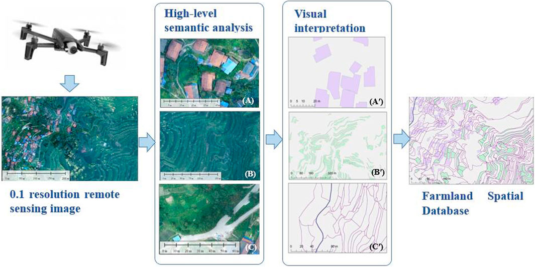
FIGURE 3. The digitalization process of cultivated land space. (A–C) are homesteads, cultivated land, and roads, respectively, and human visual interpretation corresponds to (A′), (B′), and (C′), respectively.

In 2020, a participatory survey was conducted among village officials and farmers in Baidu Village. Based on a basic understanding of the village situation through interviews with village chiefs and group leaders, a stratified random sample of farmers in different village groups was interviewed, and 171 valid questionnaires were obtained. Through the on-site identification of farmers and questionnaire interviews, we obtained information on the ownership of the completed numbered residential and farmland plots, the composition of the farmers, the current status of farmland utilization, and the input of production materials and labor. We compared the acquired information on the ownership of farmers’ residential bases with the corresponding arable land plots and evaluated the utilization of the plots one by one. Combined with the aforementioned spatial information database of cultivated land, we constructed a database of residential bases and cultivated land use tenure and spatial information of farmers in Baidu Village.

Results

Descriptive statistics of farm household survey data

According to the basic characteristics of the plots of the sample farmers in Baidu Village (Table 1), the scale of farmers’ operations is relatively small, the area of plots is small, and the LF is serious. Table 1 shows the average value of the total arable land of farmers was 0.356 hm² and the smallest farmland area was only 0.019 hm²; the average value of farming plot area was 0.041 hm² and the smallest plot area was 0.001 hm²; and the average value of farming plot was 8.72, the largest plot was 23, and the smallest plot was 2. In addition, the spatial distribution of arable land varied greatly. The mean value of elevation difference between farmers’ homesteads and plots was −48.282 m; the minimum value was −462.297 m, and the maximum value was 341.27 m. The mean value of the road network distance from farmers’ homesteads to their plots was 1831.696 m, and the minimum value reached 46.233 m. It was evident that the village did not have a concentrated distribution of home sites and plots, with long distances for farming and high commuting costs.

TABLE 1

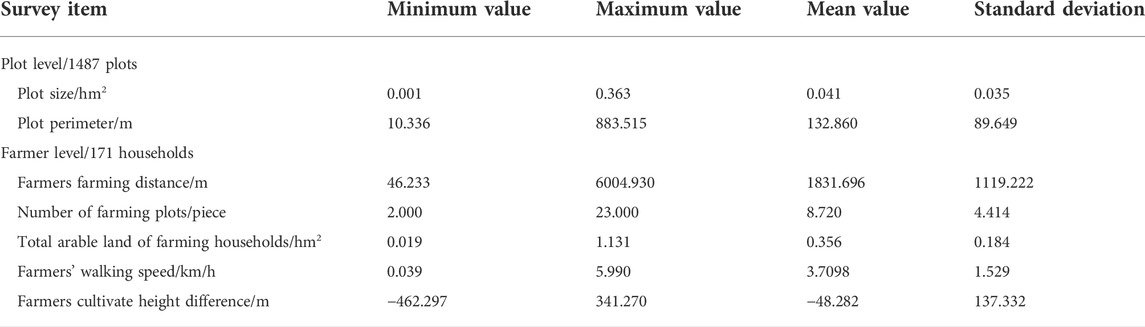
TABLE 1. Descriptive statistics of farming household survey data.

According to the Tobler function, we know that the walking speed was not directly proportional to the slope (Figure 4); when the slope value was less than 0, it is downhill. When the slope was −5%, the walking speed reached a maximum value of 5.999 km/h. When the slope was 0 (i.e., flat), the walking speed was 5 km/h. This result showed that either uphill or downhill slope had an effect on walking speed. Taking the most normal human walking speed, which is 5 km/h on level ground, as the node, walking speed became faster when −10.136% < α < 0, slowed down when α > 0, and hindered walking speed when α < −10.136%. Thus, slope directly affected walking speed and had a significant impact on travel time to work. Considering the slope of the terrain and network distance, the one-way traveling time of commuting from the farmer’s homestead to the farming plot (Figure 5) showed that the traveling time of 0.12 h was mostly near the homestead with a comparable slope and closer distance; however, the traveling time increased as the slope between the homestead and the farming plot increased and the distance was longer.

FIGURE 4

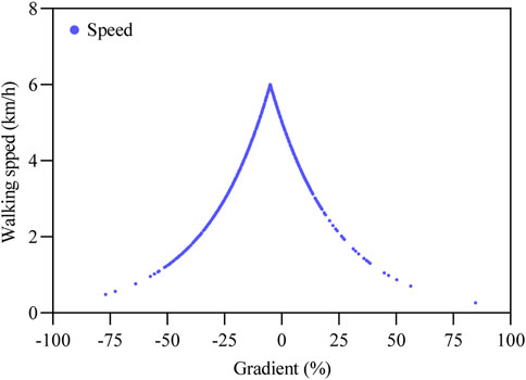
FIGURE 4. Walking speed and pace by gradient per Tobler (1993) hiking function.

FIGURE 5

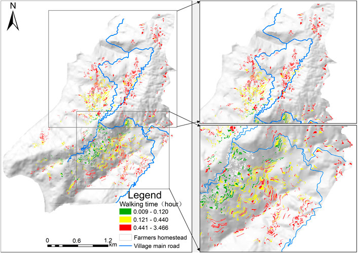
FIGURE 5. Homestead to plot walking time.

Land fragmentation of farmer

To quantitatively analyze the relationship between the status quo values of each index and the index of fine fragmentation of farmland, we selected the index of fine fragmentation of farmland in Baidu Village as the dependent variable (y), and selected the accessibility of farm plots (x₁), the index of farm plot area (x₂), and the index of farm plot shape (x₃) as independent variables. We conducted the regression analysis one by one (Figure 6). Each indicator (x₁, x₂, x₃) was linearly and positively correlated with FLFI (y), and the regression coefficients were 1.344, 1.736, and 0.8274. The coefficients of determination R were 0.748, 0.653, and 0.055, the correlation coefficients r were 0.865, 0.808, and 0.236. The two-sided significance test probability p values were less than 0.05. The best fit and the highest correlation were found between the road accessibility index of farm plots and the index of cultivated LF; the correlation between the index of farm plot shape and the index of cultivated LF was lower. The fitted regression equations were as follows:

${\mathrm{y}=1.344\mathrm{x}}_1+1.292(12)$

${\mathrm{y}=1.736\mathrm{x}}_2+0.2276(13)$

${\mathrm{y}=0.8274\mathrm{x}}_3+1.217(14)$

FIGURE 6

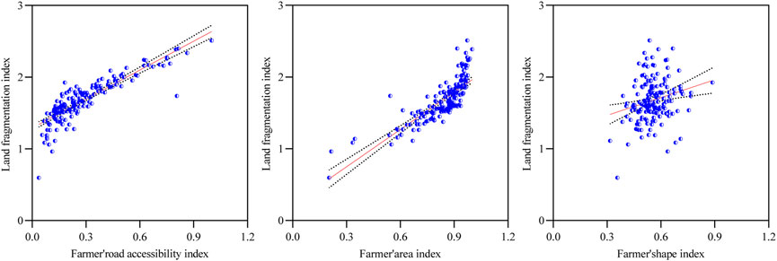
FIGURE 6. Correlation analysis on FLFI.

We identified the relationship between each evaluation index and FLFI using geographic probes, and the impact measures q of F1, F2, and F3 on FLFI were 0.692, 0.617, and 0.085, respectively. Thus, the road accessibility index of farm plots was the most influential indicator on FLFI, followed by the area index of farm plots, and finally the shape index of farm plots. The results of the correlation analysis and the geographic detector showed no significant differences in the effects of each indicator on FLFI, which indicated that the results of the analysis have good reliability and objectivity.

Land fragmentation of village

Based on Eq. 2, the VLFI of Baidu Village was 1.678. Equation 1 was used to calculate FLFI (Figure 7) of each farm household in Baidu Village in 2020. With the increase in FLFI, the number of farm households showed an olive shape, increasing first and then decreasing. The cultivated FLFI of farm households was concentrated between 1 and 2, with total 150 households accounting for 87.72% of all farm households, among which 20 households were larger than 2, and only 1 household had FLFI of less than 1.

FIGURE 7

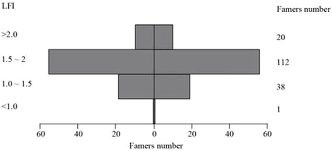
FIGURE 7. Correlation analysis on FLFI.

Comparative analysis of different plot road accessibility index models

From the correlation analysis and geographic detector synthesis, we concluded that the farm road accessibility index was the dominant factor. To compare the accuracy of the existing F1 index model, we compared the measurement model that considers the natural features of the ground and the road network with the model that does not consider the influence of the terrain and the road network. To make the road accessibility index more intuitive to better reflect the convenience of road commuting for farmers, we instead of applying the farmer road accessibility index (F₁) normalized by the maximum value, the road accessibility value (f₁), which directly reflects commuting time, was used. Three major models were compared and analyzed: Model A refers to the traveling time under the consideration of the terrain and road network distance—that is, the new measurement model proposed in this paper. Model B refers to the traveling time under the consideration of the terrain influence but not the road network distance using the straight-line distance. Model C refers to the traveling time under the consideration of the road network distance but not the terrain influence (Ge and Zhao, 2019).

The results obtained from these three farm-road-accessibility-evaluation models followed a similar trend (Figure 8). Table 2 shows the difference between these three indices was that model A obtained a higher value of 902.790, with a minimum value of 33.38 and a mean value of 258.498. Model B obtained a lower value of 21.83, and its maximum value was also the smaller of the three major models at 612.63, with a mean value of 163.015. The minimum value of model C was greater than models A and B at 41.32, and the maximum value was greater than model B but less than model A at 750.48, with a mean value of 218.479. Therefore, the accuracy of model B for measuring the road accessibility index in mountainous areas was much lower than that of models A and C. In contrast, the lowest values of both model A and model C were found in the same farmer, and model C was 7.94 smaller than model A. The maximum slope between the cultivated land and the homestead of this farmer was −6.441%, which was located in the downhill direction of the homestead, and the slope was equivalent to a slightly downhill walk, where the speed was slightly higher compared to the flat land (Figure 4). The speed of model A was 95 m/min (Figure 2), and the speed of model C was 83.330 m/min. The speed of model A was greater than that of model C. Model A considered the walking speed under the influence of terrain, whereas the speed of model C was a constant value without considering the influence of terrain. In addition, the difference between the two maximum values of 152.31 appeared in the same farmer (Table 3). This farmer has 21 plots of land, and plot 4 has a large difference between the two models’ results. The plot and the farmer’s home base slope had a difference of 31.264%, the speed of model A was 1.696 km/h (28.267 m/min), and the speed of model C was a constant value of 83.33 m/min. Model C did not take into account that uphill would slowed down the walking speed and the speed was constant, which was not consistent with the actual situation. Model A was take into account the resistance of road slope to walking, which slowed down the walking speed and greatly increased the traveling time of the farmer. This resistance was enhanced when the distance was larger. The road accessibility index that considered the slope of the terrain and the distance of the road network provided a more accurate portrayal.

FIGURE 8

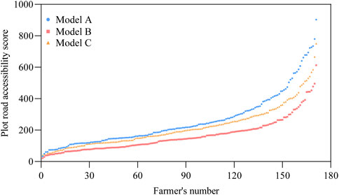
FIGURE 8. Comparison of the values of the three plot road accessibility indices.

TABLE 2

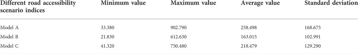
TABLE 2. Results of three road accessibility scenarios.

TABLE 3

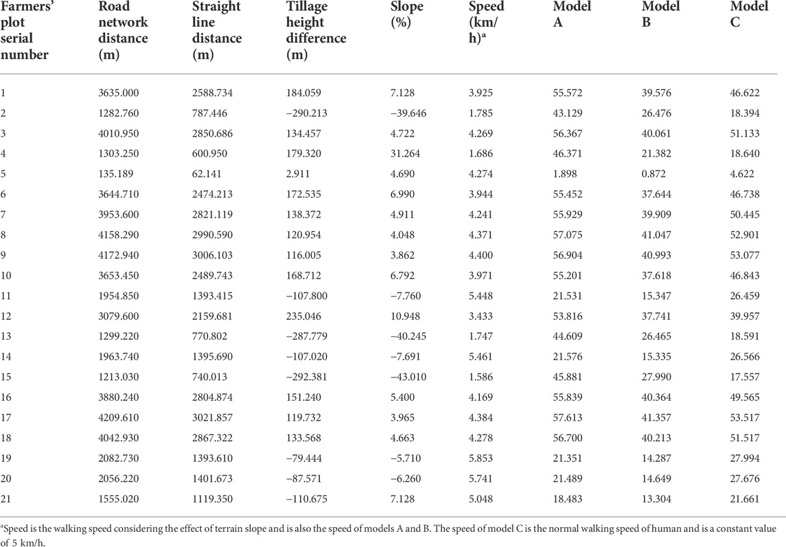
TABLE 3. Farmer sample data.

According to these results, we found that the road accessibility indicators of models B and C both underestimated the degree of road accessibility. First, the distance of model B was Euclidean distance, which underestimated the distance from the homestead to the plot. Second, the walking speed of model C did not consider the influence of topography, which was limited by the topography in mountainous areas with large topographic relief and directly affected the commuting time of farmers. Therefore, when measuring the degree of LF, the Model A that integrated terrain slope and road network better portrayed the real situation.

Discussion

In this study, we constructed a new LF measurement model based on topographic slope and road network. This model can more accurately determine the LF of farmers so that decision-makers can accurately implement land management policies. Currently, there are two major perspectives for determining the degree of LF, one is based on the mesoscale regional landscape perspective (Liu et al., 2019), which expands the concept of fractionalization to the scale of landscape ecology and focuses on the degree of fragmentation of land use types in surface patches. It ignores the presence of multiple farmer operators in a landscape patch. Another one is based on the micro-scale farmer’s perspective and takes the basic unit plot of the farmer’s farming operation as the object of study. Since the main agricultural operators in China are farmers and the land is mainly contracted and operated by farmers, the LF measurement model is more relevant to the actual situation based on the micro-scale farmers’ perspective. The current micro-level indicators mainly include the number of parcels, parcel area, shape, and the influence of the degree of dispersion (Niroula and Thapa, 2005; Demetriou et al., 2013; Lu et al., 2018), through correlation analysis, the results indicate that the indicator of plot dispersion carved using road accessibility is the dominant factor, i.e., the commuting time of the farmer to the homestead, scholars considered the road network distance to break through the error generated by previous studies using straight-line distance (Ge and Zhao, 2019), but did not consider the impact of terrain slope on speed, walking speed of 5 km/h and a constant value, which is not consistent with the actual situation. This study integrates surface natural elements and road network distances to consider walking speed under the influence of topography. Figure 9 shows three different scenarios of road accessibility are compared, Figure 9A shows the scenario considering the terrain slope and the road network, i.e., the scenario presented in this paper. Figure 9B is the scenario considering terrain slope without road network. Figure 9C is the scenario proposed by scholars considering the distance of road network but not the slope of the terrain. The final result indicates that the new measure proposed in this paper further portrays the degree of dispersion of farmers’ plots.

FIGURE 9

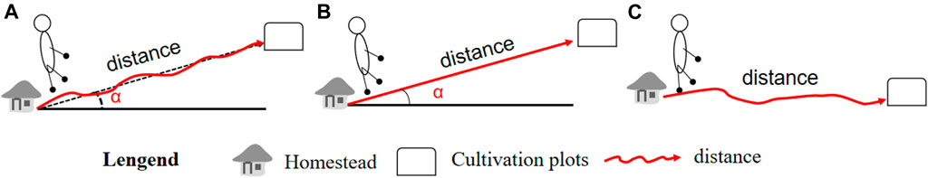
FIGURE 9. Road accessibility index for three different scenarios. (A) indicates a scenario where road network distances and terrain slope are considered, (B) indicates a scenario where straight-line distances and terrain slope are considered, and (C) indicates a scenario where road network distances are considered but terrain slope is not considered.

To mitigate the effects of LF, in the context of China’s strong advocacy of agricultural modernization, mountainous areas have focused on improving agricultural infrastructure, including the construction of farming road networks, such as machine roads. As a result, the costs of farm commuting, material transportation, and machinery running time have decreased and agricultural mechanization and production efficiency have increased. At the same time, when the slope between the homestead and the plot is large and the distance is far away, the input and income costs are integrated, and land transfer and engineering management measures are comprehensively used for plots that have better quality, promoting the moderate-scale operation of agriculture. In this study, to accurately extract the spatial information of farmers’ homesteads, plots, and road networks, remote sensing data must have high accuracy, which requires UAV remote sensing images and high-precision satellite images. Thus, understanding how to obtain high-resolution images of large areas must be further explored.

Conclusions

Decision-makers need an accurate and comprehensive model to quantify LF. We selected three indicators for inclusion in the model: the road accessibility index of farm plots, the area index of farm plots, and the shape index of farm plots. We used resolution of 0.1 m remote sensing images and farm household survey data to build a village road network and constructed a database of farm household residential bases and farmland use tenure and spatial information in Baidu Village. The topography was incorporated into the metrological model, including the calculation of slope and pedestrian walking speed. By obtaining the elevation of the homestead and the plot, the shortest distance from the farmer’s homestead to the corresponding plot, we determined the slope of the homestead and the corresponding plot. By portraying the farmer’s walking speed under the slope image, we obtained accurate geospatial data for the model and measured the degree of arable LF in Baidu Village. The results showed that it is necessary to create a road network of house bases and cultivated land in Baidu Village and to calculate the slope perception of pedestrian accessibility. By measuring the degree of cultivated LF while considering the walking speed of farmers with slope, we obtained an effective model to measure cultivated LF.

The LF model generated by the model integrating speed under the influence of road network distance and terrain slope had the following characteristics: it integrated the three core LF factors and was comprehensive; and it was flexible and context-specific, as the model was applicable in both mountainous and plain areas. Applying the model in an empirical study and comparing the results with two existing indicators, the results showed that the existing indicators underestimated (or overestimated) the degree of LF because they ignored the important variable of topographic slope. Therefore, the existing indicators may provide misleading results for decision making. In contrast, we verified that the present model provides a more reliable and robust measure of LF, performing significantly better than existing indices.

Data availability statement

The original contributions presented in the study are included in the article/Supplementary Material, further inquiries can be directed to the corresponding author.

Author contributions

YZ: Conceived the research ides. LS: Data curation and writing original draft. ML: Review and editing. XL: Supervision and methodology.

Funding

This work was supported by the Natural Science Foundation of Guizhou Province, China (No. ZK (2021)YIBAN184), and the National Natural Science Foundation of China (No. 41771115).

Acknowledgments

We are so grateful to our reviewers Wiwin Ambarwulan and Shaoquan Liu for their important comments, which have helped us to improve the manuscript.

Conflict of interest

The authors declare that the research was conducted in the absence of any commercial or financial relationships that could be construed as a potential conflict of interest.

Publisher’s note

All claims expressed in this article are solely those of the authors and do not necessarily represent those of their affiliated organizations, or those of the publisher, the editors and the reviewers. Any product that may be evaluated in this article, or claim that may be made by its manufacturer, is not guaranteed or endorsed by the publisher.

Supplementary material

The Supplementary Material for this article can be found online at: https://www.frontiersin.org/articles/10.3389/fenvs.2022.1017599/full#supplementary-material

References

Aghabayk, K., Parishad, N., and Shiwakoti, N. (2021). Investigation on the impact of walkways slope and pedestrians physical characteristics on pedestrians normal walking and jogging speeds. Saf. Sci. 133, 105012. doi:10.1016/j.ssci.2020.105012

CrossRef Full Text | Google Scholar

Ali, D. A., and Deininger, K. (2015). Is there a farm-size productivity relationship in african agriculture?:evidence from Rwanda. Land Econ. 91 (2), 317–343. doi:10.3368/le.91.2.317

CrossRef Full Text | Google Scholar

Bettinger, P., Bradshaw, G. A., and Weaver, G. W. (1996). Effects of geographic information system vector–raster–vector data conversion on landscape indices. Can. J. For. Res. 26, 1416–1425. doi:10.1139/x26-158

CrossRef Full Text | Google Scholar

Blarel, B., Hazell, P., Place, F., and Quiggin, J. (1992). The economics of farm fragmentation: Evidence from Ghana and Rwanda. World Bank. Econ. Rev. 6, 233–254. doi:10.1093/wber/6.2.233

CrossRef Full Text | Google Scholar

Carter, M. R., and Yao, Y. (2002). Local versus global separability in agricultural household models: The factor price equalization effect of land transfer rights. Am. J. Agric. Econ. 84, 702–715. doi:10.1111/1467-8276.00329

CrossRef Full Text | Google Scholar

de Garis De Lisle, D. (2010). Effects of distance on cropping patterns internal to the farm. Ann. Assoc. Am. Geogr. 72, 88–98. doi:10.1111/j.1467-8306.1982.tb01385.x

CrossRef Full Text | Google Scholar

del Corral, J., Perez, J. A., and Roibas, D. (2011). The impact of land fragmentation on milk production. J. Dairy Sci. 94, 517–525. doi:10.3168/jds.2010-3377

PubMed Abstract | CrossRef Full Text | Google Scholar

Demetriou, D., Stillwell, J., and See, L. (2013). A new methodology for measuring land fragmentation. Comput. Environ. Urban Syst. 39, 71–80. doi:10.1016/j.compenvurbsys.2013.02.001

CrossRef Full Text | Google Scholar

Di Falco, S., Penov, I., Aleksiev, A., and van Rensburg, T. M. (2010). Agrobiodiversity, farm profits and land fragmentation: Evidence from Bulgaria. Land Use Policy 27, 763–771. doi:10.1016/j.landusepol.2009.10.007

CrossRef Full Text | Google Scholar

Ge, Y., and Zhao, Y. (2019). Improvement of farmland fragmentation measurement model based on road network analysis. Resour. Sci. 41, 766–774. doi:10.18402/resci.2019.04.13

CrossRef Full Text | Google Scholar

Gónzalez, X. P., Marey, M. F., and Álvarez, C. J. (2007). Evaluation of productive rural land patterns with joint regard to the size, shape and dispersion of plots. Agric. Syst. 92, 52–62. doi:10.1016/j.agsy.2006.02.008

CrossRef Full Text | Google Scholar

Hess, D. B., and Almeida, T. M. (2007). Impact of proximity to light rail rapid transit on station-area property values in buffalo, New York. Urban Stud. 44 (5/6), 1041–1068. doi:10.1080/00420980701256005

CrossRef Full Text | Google Scholar

Higgins, C. D. (2019). A 4D spatio-temporal approach to modelling land value uplift from rapid transit in high density and topographically-rich cities. Landsc. Urban Plan. 185, 68–82. doi:10.1016/j.landurbplan.2018.12.011

CrossRef Full Text | Google Scholar

Igozurike, M. U. (1974). Land tenure, social relations and the analysis of spatial discontinuity. Area 6, 132–135.

Google Scholar

Janus, J., Mika, M., Leń, P., Siejka, M., and Taszakowski, J. (2016). A new approach to calculate the land fragmentation indicators taking into account the adjacent plots. Surv. Rev. 50, 1–7. doi:10.1080/00396265.2016.1210362

CrossRef Full Text | Google Scholar

Januszewski, J. (1968). Index of land consolidation as a criterion of the degree of concentration. Geogr. Pol. 14, 291–296.

Google Scholar

Kawasaki, K. (2010). The costs and benefits of land fragmentation of rice farms in Japan. Aust. J. Agric. Resour. Econ. 54, 509–526. doi:10.1111/j.1467-8489.2010.00509.x

CrossRef Full Text | Google Scholar

Kawasaki, K. (2011). The impact of land fragmentation on rice production cost and input use. Jpn. J. Rural Econ. 13, 1–14. doi:10.18480/jjre.13.1

CrossRef Full Text | Google Scholar

Latruffe, L., and Piet, L. (2014). Does land fragmentation affect farm performance? A case study from brittany, France. Agric. Syst. 129, 68–80. doi:10.1016/j.agsy.2014.05.005

CrossRef Full Text | Google Scholar

Lee, S. H., Goo, S. H., Chun, Y. W., and Park, Y. J. (2015). The spatial location analysis of disaster evacuation shelter for considering resistance of road slope and difference of walking speed by age - case study of seoul, korea. J. Korean Soc. Geospatial Inf. Syst. 23, 69–77. doi:10.7319/kogsis.2015.23.2.069

CrossRef Full Text | Google Scholar

Liu, J., Jin, H., Xu, W., Sun, R., Han, B., Yang, X., et al. (2019). Influential factors and classification of cultivated land fragmentation, and implications for future land consolidation: A case study of Jiangsu Province in eastern China. Land Use Policy 88, 104185–104185. doi:10.1016/j.landusepol.2019.104185

CrossRef Full Text | Google Scholar

Lu, H., Xie, H., He, Y., Wu, Z., and Zhang, X. (2018). Assessing the impacts of land fragmentation and plot size on yields and costs: A translog production model and cost function approach. Agric. Syst. 161, 81–88. doi:10.1016/j.agsy.2018.01.001

CrossRef Full Text | Google Scholar

Masini, E., Barbati, A., Bencardino, M., Carlucci, M., Corona, P., and Salvati, L. (2018). Paths to change: Bio-economic factors, geographical gradients and the land-use structure of Italy. Environ. Manag. 61, 116–131. doi:10.1007/s00267-017-0950-0

PubMed Abstract | CrossRef Full Text | Google Scholar

Nair, P. K. R. (2014). Grand challenges in agroecology and land use systems. Front. Environ. Sci. 2, 1. doi:10.3389/fenvs.2014.00001

CrossRef Full Text | Google Scholar

Nguyen, T., Cheng, E., and Findlay, C. (1996). Land fragmentation and farm productivity in China in the 1990s. China Econ. Rev. 7, 169–180. doi:10.1016/s1043-951x(96)90007-3

CrossRef Full Text | Google Scholar

Niroula, G. S., and Thapa, G. B. (2005). Impacts and causes of land fragmentation, and lessons learned from land consolidation in South Asia. Land Use Policy 22, 358–372. doi:10.1016/j.landusepol.2004.10.001

CrossRef Full Text | Google Scholar

Niroula, G. S., and Thapa, G. B. (2007). Impacts of land fragmentation on input use, crop yield and production efficiency in the mountains of Nepal. Land Degrad. Dev. 18, 237–248. doi:10.1002/ldr.771

CrossRef Full Text | Google Scholar

Páez, A., Scott, D. M., and Morency, C. (2012). Measuring accessibility: Positive and normative implementations of various accessibility indicators. J. Transp. Geogr. 25, 141–153. doi:10.1016/j.jtrangeo.2012.03.016

CrossRef Full Text | Google Scholar

Qi, X., and Dang, H. (2018). Addressing the dual challenges of food security and environmental sustainability during rural livelihood transitions in China. Land Use Policy 77, 199–208. doi:10.1016/j.landusepol.2018.05.047

CrossRef Full Text | Google Scholar

Simmons, A. J. (1964). An index of farm structure, with a Nottinghamsire example. East Midl. Geogr. 3, 255–261.

Google Scholar

Tan, S., Heerink, N., and Qu, F. (2006). Land fragmentation and its driving forces in China. Land Use Policy 23, 272–285. doi:10.1016/j.landusepol.2004.12.001

CrossRef Full Text | Google Scholar

Tan, S., Heerink, N., Kuyvenhoven, A., and Qu, F. (2021). Impact of land fragmentation on rice producers’ technical efficiency in South-East China. NJAS Wageningen J. Life Sci. 57, 117–123. doi:10.1016/j.njas.2010.02.001

CrossRef Full Text | Google Scholar

Tobler, W. (1993). Three presentations on geographical analysis and modeling: Non- isotropic geographic modeling; speculations on the geometry of geography; and global spatial analysis. Ncgia Technical Reports. Available at: https://escholarship.org/uc/item/05r820mz.

Google Scholar

UNDESA (2014). World urbanization prospects: The 2014 revision, highlights. New York: United Nations.

Google Scholar

United Nations Population Division (2011). World population prospects: The 2010 revision. Available at: http://esa.un.org/unpd/wpp/index.htm.(Accessed June 18, 2022).

Google Scholar

Van Hung, P., MacAulay, T. G., and Marsh, S. P. (2007). The economics of land fragmentation in the north of Vietnam. Aust. J. Agric. Resour. Econ. 51, 195–211. doi:10.1111/j.1467-8489.2007.00378.x

CrossRef Full Text | Google Scholar

Wan, G. H., and Cheng, E. (2001). Effects of land fragmentation and returns to scale in the Chinese farming sector. Appl. Econ. 33, 183–194. doi:10.1080/00036840121811

CrossRef Full Text | Google Scholar

Wang, W. M., and Wang, Q. (2010). Land use planning: Land use planning. Beijing: Science Press.

Google Scholar

Wang, J. F., and Xu, C. D. (2017). Geodetectors: Principles and prospects. Acta Geogr. Sin. 72, 19. doi:10.11821/dlxb201701010

CrossRef Full Text | Google Scholar

Zhao, K. (2011). Land fragmentation and its quantitative measurement method. China Land Sci. 25, 15–31. doi:10.13708/j.cnki.cn11-2640.2011.10.005

CrossRef Full Text | Google Scholar