 Fanyu Meng1
 Jilin Gu
 Ling-en Wang
95% of researchers rate our articles as excellent or good
Learn more about the work of our research integrity team to safeguard the quality of each article we publish.
Find out more
ORIGINAL RESEARCH article
Front. Environ. Sci. , 10 November 2022
Sec. Environmental Informatics and Remote Sensing
Volume 10 - 2022 | https://doi.org/10.3389/fenvs.2022.1014856
This article is part of the Research Topic Meta-Scenario Computation for Social-Geographical Sustainability View all 60 articles
In order to predict sea surface temperature (SST), combined with the genetic algorithm and the least-squares method, a GM(1,1|sin) power model prediction method based on similarity deviation is proposed. We first combined the data of two consecutive years into a new time series, analyzed the similarity of the data of the previous year, and obtained the most similar year and the corresponding new time series. Then, we established a GM(1,1|sin) power model to predict SST. In model validation, we predicted the monthly average SST from 2016 to 2020 with the data from 1985 to 2015, 2016, 2017, 2018, and 2019. The validation results showed that the maximum mean relative error (MRE) was 13.28%, the minimum MRE was 5.54%, and the average MRE and the root mean square error (RMSE) were 9.81% and 1.0627, respectively. All of evaluation metrics of Lin’s concordance correlation coefficient (LCCC) and the ratio of performance to deviation (RPD) were excellent. We iteratively predicted the monthly average SST from 2016 to 2020 with the data from 1985 to 2015, the maximum MRE was 13.91%, the minimum was 7.80%, and the average MRE, RMSE, LCCC and RPD are 11.07% 1.0603, 0.9894, and 7.497, respectively. Compared with GM(1,1), GM(1,1|sin + cos), and GM(1,1|sin) models, the proposed model outperformed these models with at least 50% in the MRE. It proves that the proposed model can be regarded as a better solution to predicting SST.
SST prediction is closely related to the daily life of human beings, and understanding the changes of SST in advance plays an important leading role in the school of fish swimming, deep sea exploration, cold wave warning, and even military defense (Shi et al., 2018).SST is one of the most important parameters in the study of global oceanic and atmospheric interactions. The prediction of SST is to predict the sea temperature field, especially the SST changes with time. Accurate prediction of SST can provide effective support for coping with marine disasters such as storms and typhoons and prevent red tide (Sun et al., 2020).
Today, more than a dozen countries have made outstanding contributions to sea water temperature prediction services. Among them, the United States, the former Soviet Union, and Japan publicly provide the largest number of sea water temperature analysis and prediction products (Wang et al., 2021). Sea water temperature prediction in China began in the early 1960s. At first, Shandong Ocean University, Shandong Marine and Fishery Research Institute, and Yantai Meteorological Institute cooperated to explore the single-station water temperature prediction method in the offshore area of Yantai. With the need of the development of marine economy, the daily average SST prediction of a single station in coastal cities and the water temperature prediction of coastal bathing beaches have been successively carried out (Zhang, 2004).
There have been many studies on the prediction of sea water temperature in recent years. Dong et al. (2008) reconstructed the time series in phase space and used a fuzzy neural network. The relative error of the predicted value was controlled within 10%, and the fitting correlation coefficient was 0.98. Jin et al. (1999) using a threshold autoregressive model selected sea surface temperature data from 1963 to May 1994 in Dalian’s Tiger Beach. The number of threshold intervals and the search range of threshold values were found by global optimization combined with a genetic algorithm. The predicted value in May 1995 was 0.58°C which was different from the measured value. Lu et al. (2009) selected CTD data of the East China Sea and the non-stationary time series were stabilized by the EMD method, and the correlation coefficient reached 0.94. He et al. (2020) selected remote-sensing data from the AVHRR satellite and adopted the periodic trend decomposition method of locally weighted regression, combined with the neural network, and the root mean square error reached 0.79°C. Kim et al. (2020) proposed a HWT prediction method based on a recursive neural network (RNN). The correlation coefficient range of prediction was from 0.9936 to 0.959, and the root mean square error range was from 0.5076°C to 1.3238°C. Wang et al. (2021) established a multi-variable artificial neural network model. The RMSE achieved based on the training results of SST was 0.348°C. Zhang et al. (2020) designed a recursive unit (GRU) neural network algorithm on the basis of gating for medium and long-term SST prediction, and its average absolute error was within the range of 0–2.5°C. Zhang et al. (2019) using EEMD obtained the eigenmode function, which solved the problem of the high signal-to-noise ratio of the results of the EMD algorithm and further improved the prediction accuracy, and the agreement degree between the predicted value and the measured value reached 99.61%. Qu et al. (2021) used the multi-scale fusion method to predict the daily mean temperature of sea water with a root mean square error of 0.996°C and also made a prediction on an hourly scale with a root mean square error of 1.06°C. Li et al. (2020) used the deep neural network based on long and short memory to achieve a root mean square error of 0.5°C in 1 month and 0.66°C in 12 months. Lu et al. (2021) used the CMIP5 model to predict the next 100 years, and the results showed that SST would increase significantly by 2100: SST would increase by about 1.55°C per decade, while seasonal SST would increase by 1.03–1.95°C. Sung et al. (2021) used the CMIP6 model to calculate the temperature around the Korean Peninsula which will increase from 0.49°C to 0.59°C every 10 years.
How to improve the accuracy of grey prediction theory in the oscillation sequence has become a topic for mathematicians. The research achievements that have made breakthroughs are mainly divided into two aspects in recent years: on the one hand, the processing of the original sequence is improved. Zhao and Wu (2010) carried out translation transformation and geometric average transformation operation on the original data sequence. Li and Liu (2020) proposed the grey interval GM(1,1) model by the upper bound sequence and the lower bound sequence of the original sequence was taken. Zeng et al. (2020) used a new-structure grey Verhulst model for predicting China’s tight gas production and the comprehensive error was 2.07%. Qian and Dang (2009) carried out accelerated translation transformation and weighted mean generation transformation of the original sequence. Cui and Liu (2012) proposed to carry out accelerated exponential transformation and geometric average generation transformation of the original sequence. On the other hand, the bleaching equation in grey prediction theory is improved, Wang and Luo (2017) used a fractional discrete GM(1,1) power model based on the GM(1,1) power model. Wang et al. (2013) carried out the power function optimization of the GM(1,1) power model, and five derived models are proposed, including the oscillating GM(1,1) power model with time-varying parameters and considering the system delay. The residual error is also predicted by using the Fourier series, which improves the grey prediction theory to certain extent. Zeng and Li (2021) introduced a new action quantity k2d and r-order was introduced into the traditional three-parameter discrete grey forecasting model. The results show that the comprehensive mean relative percentage error of the new model was 0.4765%. In this study, the GM(1,1|sin) power model is selected to estimate the SST.
To minimize the impact of the cold snap on the SST prediction, we used data from 1985 to 2020 to predict the SST for the next 50 years. However, these 35 years of data are not sufficient to predict temperature trends over the next 50 years. In view of the current situation, we designed a grey prediction model to obtain more reliable data to successfully overcome the problem resulting from insufficient data. Grey prediction theory is a kind of the dynamic model which uses discrete data to establish a differential equation based on the concepts of correlation space, smooth discrete functions, and so on. The equation is named as the grey model (GM) that generates discrete random numbers into numbers whose randomness is significantly weakened and more regular, so that it is convenient to study and describe the process of its change. The GM has a strict theoretical foundation and advantage of practicality. Therefore, the results of the grey prediction model are relatively stable, which is not only applicable to the prediction of large data amount, but also accurate when the data amount is small (Zeng et al., 2020).The GM is a powerful method for the problems characterized by samples with uncertainty. By identifying different degrees of development trends among system factors, the GM generates strong regularity of data sequences and then establishes the corresponding differential equation model to predict the future trend. The GM holds that the behaviors of systems are in order for the purpose of the implementation of a certain function, although they seem hazy and complex (Yin, 2017). The traditional GM(1,1) prediction curve is approximate to a straight line, so it can only be predicted for some monotonic increasing or decreasing sequences. The prediction of the sea water temperature with strong fluctuation of vibration is not suitable for GM(1,1) (Tang et al., 2008). Zeng, 2019 established a GM(1,1|sin) power model based on the GM(1,1|sin) model to solve the compound oscillation sequence with different periods.
The purpose of this study was to use the experience predict method to establish a prediction model of SST which can be easily implemented and applied, a GM(1,1|sin) power model prediction method based on similarity deviation was proposed. We first combined the data of two consecutive years into a new time series, analyzed the similarity of the data of the previous year, and obtained the most similar year and the corresponding new time series. Then, we established a GM(1,1|sin) power model to predict SST. Based on the MATLAB simulation, this method used data from 1985 to 2015, a total of 372 monthly average SST to predict data of 2016–2020, and compared with the measured data, then predicted the SST of the 50 years after 2020, and drew conclusions.
The SST series is a kind of a time series. A time series refers to the sequence formed by arranging the values of a variable at different times in time sequence, and its time scale can be a day, month, year, hour, etc. The time series model is a mathematical model established by using the time series. It is mainly used for short-term prediction of the future and belongs to the trend predicting method. In reality, the vast majority of phenomena are rapidly changing. With the passage of time, the internal and external influencing factors change greatly, which reduces the prediction accuracy gradually. The method of time series analysis and prediction predicts the future according to the development trends and change rules of past and present, which can only make effective predictions in a relatively short period of time.
The SST data used in this study are reanalysis data and measured data from the National Data Center for Marine Science. The data are from the Northwest Pacific Ocean Reanalysis Product (CORA V1.0). The product elements include sea surface height, temperature, salinity, and currents. The sea area ranges from 99°E to 150°E and 10°S to 52°N, the spatial horizontal grid resolution is 0.5° × 0.5°, and the number of the vertical layer is 35. The length of time is 60 years from January 1958 to December 2018, and the time resolution is the monthly average of the past years. The spatial horizontal grid resolution of the measured data is 0.125° × 0.125°, which is the same as that of the reanalyzed data. The time span is 5 years from 2016 to 2020, and the time resolution is the daily average. If there is a null value in the data set, the cubic spline interpolation method is used for complement.
The product was developed based on the ocean reanalysis system of the Northwest Pacific Ocean, and the ocean dynamic model of the system was the Princeton Ocean Model with the Generalized Coordinate System (POMGCS). The meteorological driving field is the NCEP meteorological reanalysis field. The ocean data assimilation method used is the multi-grid three-dimensional variational ocean data assimilation method. The assimilated ocean observations include in situ temperature and salinity observations, satellite remote sensing sea surface height anomaly (SSHA), and sea surface temperature (Reynolds SST) data. National Marine Science data in the heart of the reanalysis data format for.nc database files is more than 67 Giga bytes, at the same time, the original file format in the actual use process is relatively complex, so it must be prepared in advance according to the requirements that will be appropriate for waters of the sea surface temperature extracted and stored as .mat format, and the read load can be used on MATLAB. This study takes the Bohai Sea as the research object and obtains the surface temperature of the Bohai Sea on a certain day, as shown in Figure 1.
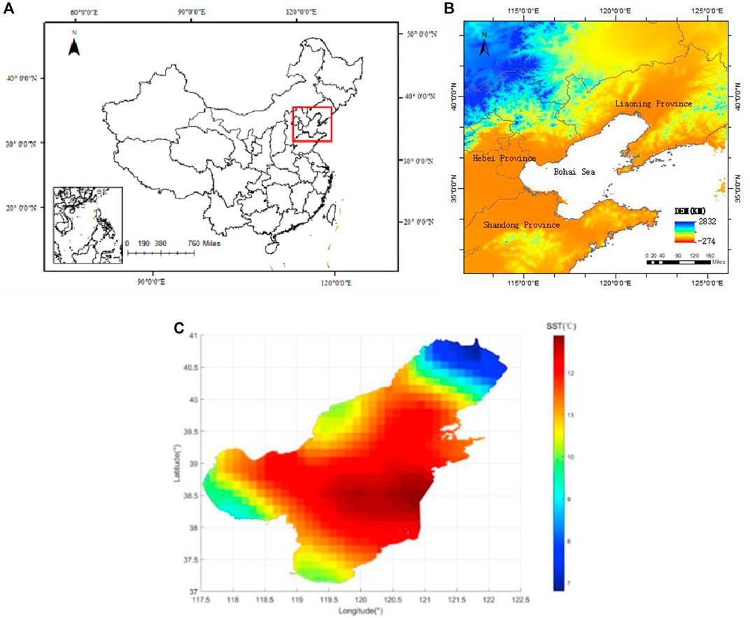
FIGURE 1. Map of China (A). Elevation map of the Bohai Sea (B). SST of the Bohai Sea (C).
As shown in Figure 2A, the observation of the SST series shows that the Bohai Sea area presents a single peak shape in the process of changing with month, that is, the maximum and minimum temperature values only appear once in every 12 months in a year. Along with the number of days in a month to promote the process of SST rendering multiple peak shapes, as shown in Figure 2B, that is, the trend of rising and falling will appear multiple times in a month. It can be seen that the variation characteristics of SST in different time scales are also different. If we observe SST on a daily scale, we can find that the change in SST is very dissimilar. If we observe SST on a monthly scale, it can be found that the SST has high similarity and obvious periodicity in different years. The similarity and periodicity of SST are conducive to the prediction of future temperature.
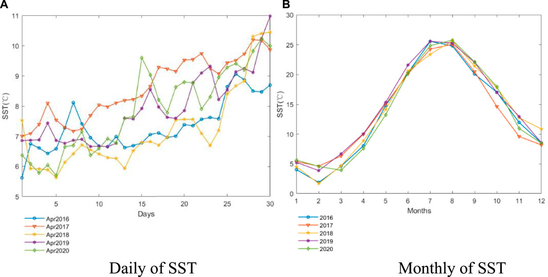
FIGURE 2. Change trend of SST in recent 5 years.
In the process of predicting the future monthly average SST, we can make use of the similarity of the data over the past years to conduct the appropriate comparison. Therefore, the metrics of similarity assessment directly determine the accuracy of SST prediction results. There are many metrics to evaluate the similarity between two samples. The similarity deviation is introduced in this study. The mean relative error (MRE), the posterior difference ratio (PDR), and the probability of small error (PSE) are the metrics to evaluate whether the prediction sequence is suitable for the real sequence and sufficient to predict in the future.
If we have two samples, A(1) is the value of the first sample, B(1) is the value of the second sample, and the total number of both samples is N. Then, the mean relative error is as follows:
The residuals between two samples
Posterior difference ratio:
where
The
The calculation formula of the probability of small error (PSE) is defined in Eq. 7. Table 1 shows the relationship between the aforementioned parameters and the grey model accuracy.
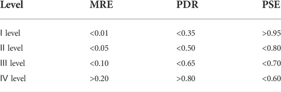
TABLE 1. Predictive model test criteria.
In addition, the root mean square error (RMSE) and MRE are selected as the evaluation parameters of prediction accuracy. The formula for RMSE is as follows:
Similarity deviation is the parameter to reflect the difference between the “shape” and “value” of two samples. The similarity deviation of these two samples can be defined as SAB.
where
In Eq. 10,
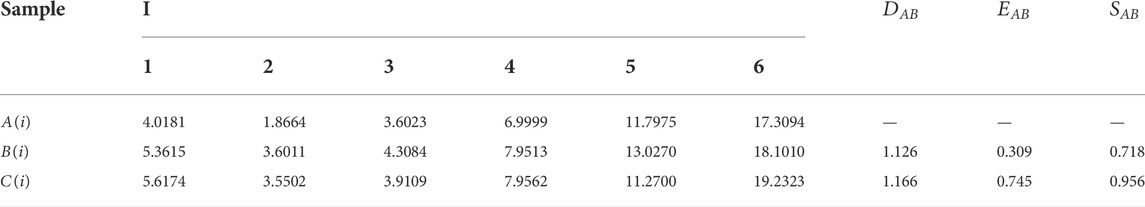
TABLE 2. Result of similarity deviation.
The Lin’s concordance correlation coefficient (LCCC) was used to evaluate the prediction model performance, because it measures the “agreement” between predicted and measured values (Zhao et al., 2021a,b).
where
Prediction accuracy was also assessed using the ratio of performance to deviation (RPD), which is calculated as the ratio of standard deviation (SD) to RMSE.
These two indexes divide the accuracy of the prediction model into four levels, as shown in Table 3.
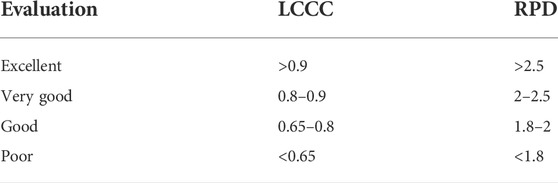
TABLE 3. Result of similarity deviation.
The original data were cumulated to get the cumulative sequence, so as to weaken the volatility and randomness of the original sequence. The new data sequence is defined as
According to the smoothness ratio test theory, the grade ratio and smoothness ratio test of SST can be defined as
When
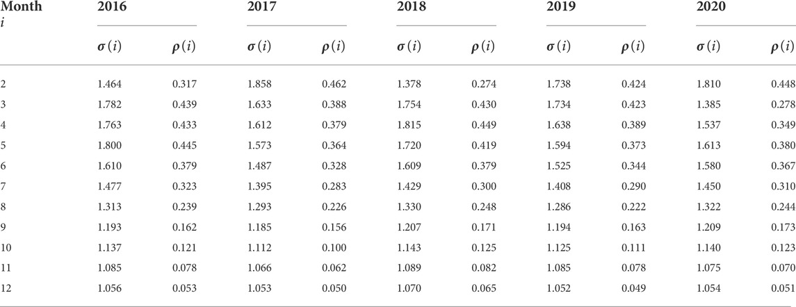
TABLE 4. Original sequence grade ratio and smoothness ratio test.
For the cumulative sequence
where
According to the cumulative sequence
The least-squares method is used to obtain the grey parameter
By putting the grey parameter
The 3/8 Simpson integral formula turns the integral into an interval sum (Shen and Zhang, 2016), and then, an approximate solution is obtained. Then, the integral is converted into
The final solution of the bleaching equation is shown as follows:
Given
With a similar predict method, the GM(1,1|sin) power model realizes the SST prediction. Therefore, this study puts forward a new method, the GM(1,1|sin) power model based on the similarity deviation. This method takes two successive years as an original sequence, combined with the similarity of the SST changes and determines the appropriate original sequence on the basis of similarity deviation, in order to solve the model parameters, then solves the grey prediction model to predict. The unknown SST of 2020 can be assumed and predicted. The data of two consecutive years (2019–2020) are first combined, and the similarity of SST changes can be used to calculate the similarity deviation between each year and 2019 according to Eq. 9. The year with the highest similarity to 2019 was found and combined with the data of the next year to form the original sequence composed of 24 data for the module to determine the model parameters, and then the prediction curve was obtained.
Table 5 shows the data of similarity deviation of each year and 2019. The changing trend is shown in Figure 3. According to the calculation results, 2016 is the year most similar to 2019.
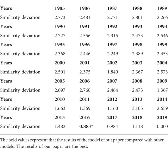
TABLE 5. Similarity deviation between all years and 2019.
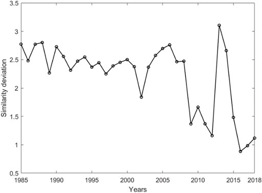
FIGURE 3. Change curve of similarity deviation.
By combining the monthly average SST from 2016 to 2017 and bringing them into the model, the bleaching equation and the evaluation metrics are obtained. The prediction model is shown in Eq. 26. The specific data are shown in Table 6 and Table 7. The average values of MRE, RMSE, LCCC, and RPD are 9.84%, 1.2363, 0.9870, and 6.0996, respectively. The evaluation metrics of LCCC and RPD were excellent based on Table 3.
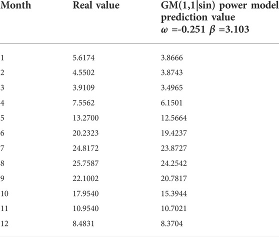
TABLE 6. Prediction results in 2020.
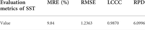
TABLE 7. Evaluation metrics of SST prediction results in 2020.
In order to eliminate the particularity of some years, the GM(1,1|sin) power model based on similarity deviation is used to predict the monthly average SST in the recent 5 years. The specific steps will not be repeated. Table 8 shows each predict year and its corresponding model. The maximum MRE is 13.28%, and the minimum is 5.54%. The 5-year MRE is 9.81%. In addition, the maximum RMSE is 1.3285, and the minimum is 0.6522. The 5-year RMSE is 1.0627, which indicates that the 5-year forecast deviated from the real value by about 1°C. All of evaluation metrics of LCCC and RPD were excellent. The specific contrast between prediction and reality is shown in Figure 4.

TABLE 8. Prediction models in 5 years.
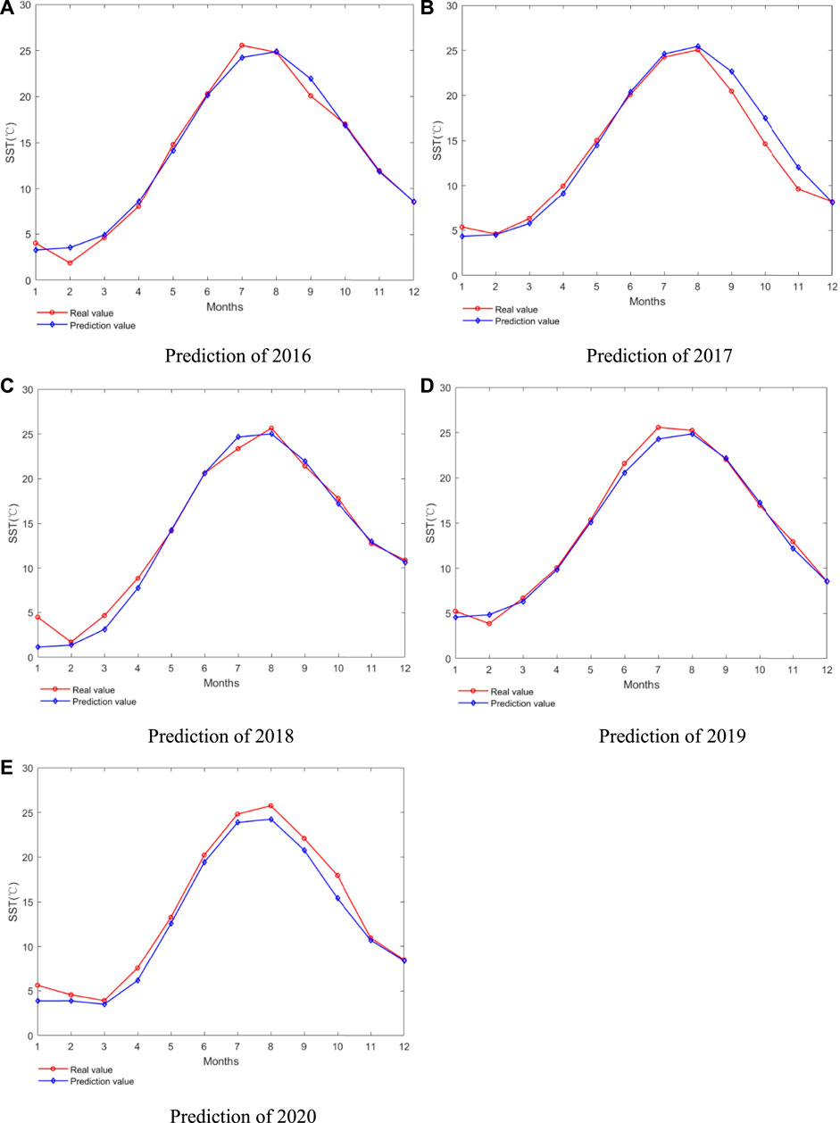
FIGURE 4. Respective prediction of the recent 5 years.
In the recent 5 years, there are 2 years in which the MRE is more than 10%, which are 2016 and 2018. Comparing the real value of these 2 years with the value of other years, the lowest temperature on record occurred in February 2018 and February 2016, and the highest temperature in 2016 occurred in July, and there was a sudden temperature change from June to August in 2018. Because the grey prediction model belongs to an autoregressive model, these abnormal temperature phenomena will directly affect the prediction results, resulting in deviation of the prediction results from the real value. In the other 3 years, due to the relatively stable temperature change, the prediction value all obtained good results. It can be seen that the factors affecting the quality of the grey prediction model are not only related to the established parameters in the model, but also related to the data of the original sequence.
We have verified the suitability of the prediction model based on the results of the monthly scale prediction. The Bohai Sea is the only inland sea in China, and it is connected to the Yellow Sea in the southeast. There are many factors influencing SST variation in this area near the land margin. In winter, due to the cold current, the temperature in the central and southeastern areas of the Bohai Sea was lower than that in other areas. Accordingly, the temperature in these areas was higher under the influence of the summer warm current.
The spatial distribution of the Bohai Sea area is represented according to the data of the monthly scale prediction in 2020, as shown in Figure 5. In January and February, the SST in the center was low and around the coastline was almost the same. The lowest was 3.88°C in the area connected with the Yellow Sea. In March, the SST was further reduced, and the temperature range was between 3.768 and 3.786. This is because the land temperature in January and February is the lowest in the year. The spatial distribution of the SST was roughly the same from April to December. The temperature rose first and then decreased, and the highest was about 25.5°C in August.
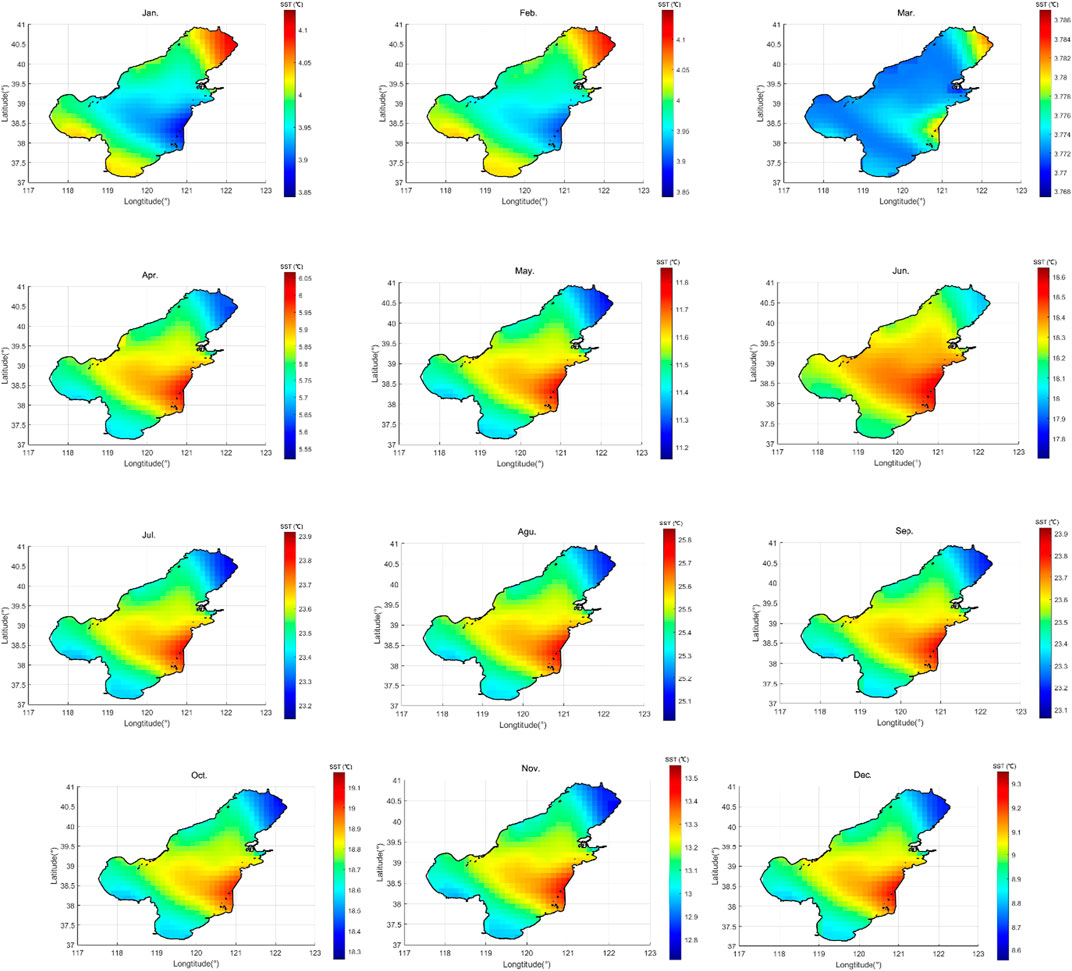
FIGURE 5. Spatial distribution of months in 2020.
This study selects a central Bohai Sea area (120°E-120.125°E and 38.5°N-38.625°N) as the research object. The monthly average SST of 2020 is selected as an original sequence. Table 9 shows the established GM(1,1|sin) power model (
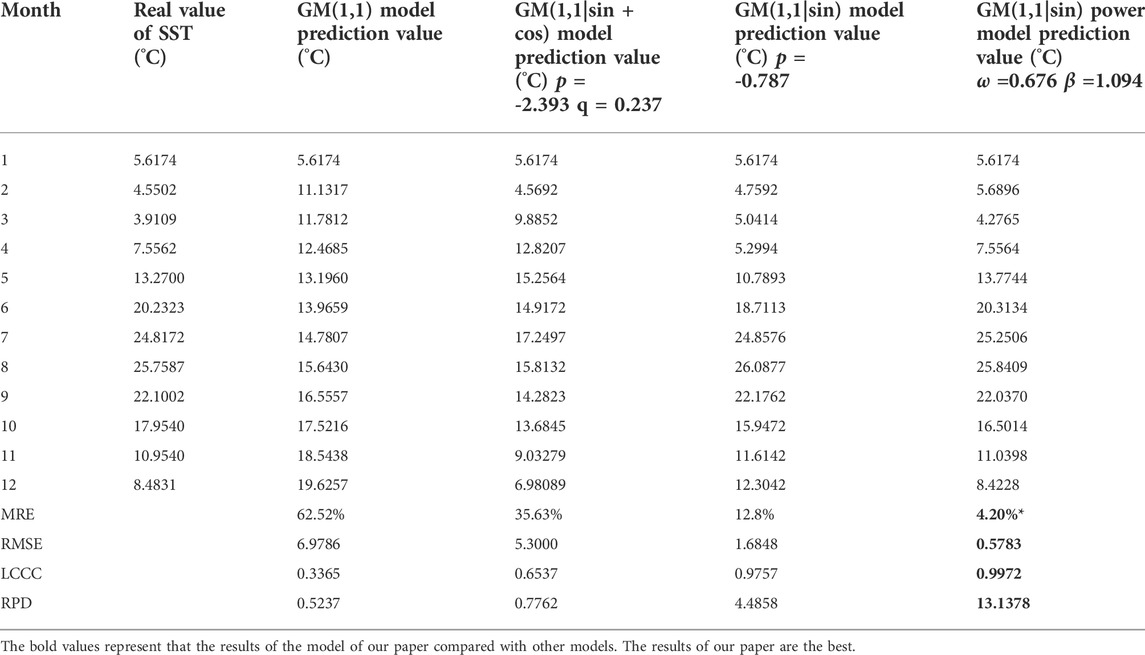
TABLE 9. Different models data of months average SST in 2020.
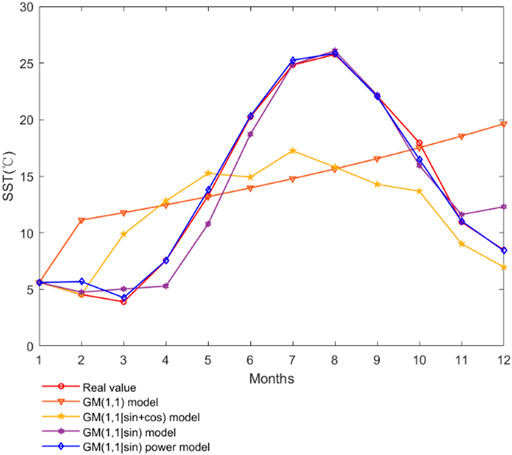
FIGURE 6. Simulation comparison chart of four models on SST.
The metrics of the four models were also obtained as shown in Table 10. The optimal model, GM(1,1|sin) power model achieves Ⅱ level accuracy standard. Each model corresponding to the relative error is shown in Figure 7A, the GM(11|sin) power model of relative error is shown in Figure 7B. The maximum and minimum relative error of GM(1,1) model are 2.01 and 0.00557, respectively. The GM(1,1|sin + cos) model corresponding relative error maximum value is 1.53, and the minimum value is 0.0042. The GM(1,1|sin) model corresponding relative error maximum value is 0.45, and the minimum value is 0.00163. The GM(1,1|sin) power model corresponding relative error maximum value is 0.25, and the minimum value is 0.00026. According to the relevant metrics PDR and PSE based on Table 1, the results proved that the GM(1,1|sin) power model can approximately reflect the monthly changes in SST.
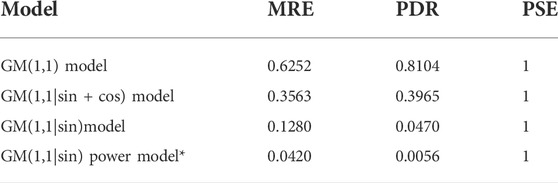
TABLE 10. Evaluation metrics of grey models in SST.
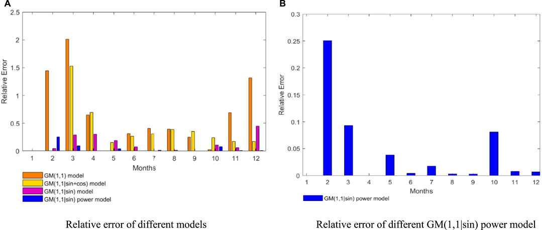
FIGURE 7. Relative error diagram.
Considering that the monthly average SST from 2016 to 2020 is to be predicted, the prediction value of 2016 will be taken as the real value after obtained, and the data will be predicted for five consecutive years by using the cycle prediction method. The results of the monthly SST prediction from 2016 to 2020 with the data from 1985 to 2015, 2016, 2017, 2018, and 2019 are shown in Table 8. The maximum MRE is 13.28%, and the minimum is 5.54%. The 5-year MRE is 9.81%. The average RMSE, LCCC, and RPD are 1.0627, 0.9897, and 7.617, respectively. The annual prediction model is shown in Table 11. The maximum value of the MRE is 13.91%, the minimum is 7.80%, and the average value is 11.07%. The average RMSE, LCCC, and RPD are 1.0603, 0.9894, and 7.497, respectively. All of evaluation metrics of LCCC and RPD were excellent. It can be seen that the prediction performance of the GM(1,1|sin) power model is stable because the deviation between the predicted value and the real value is very close in the respective prediction and consecutive prediction. The specific contrast between prediction and real is shown in Figure 8.
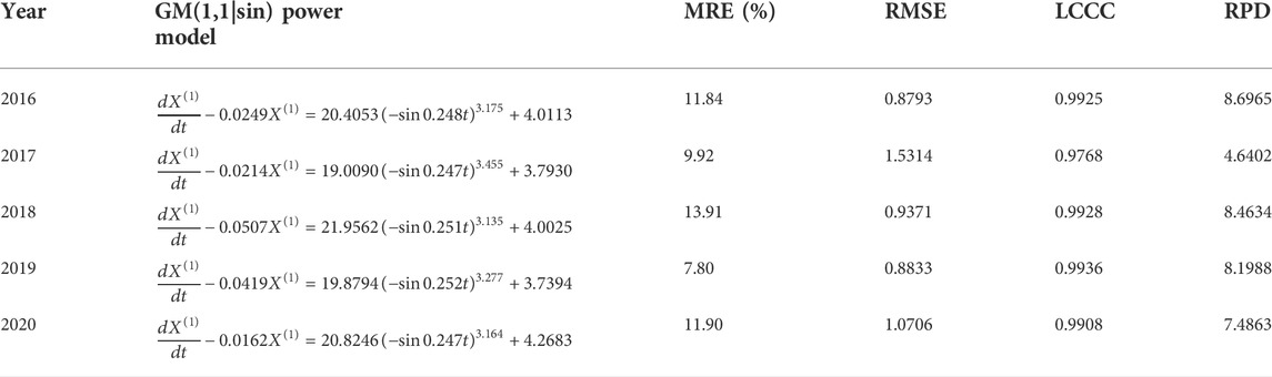
TABLE 11. Adjusted prediction models in 5 years.
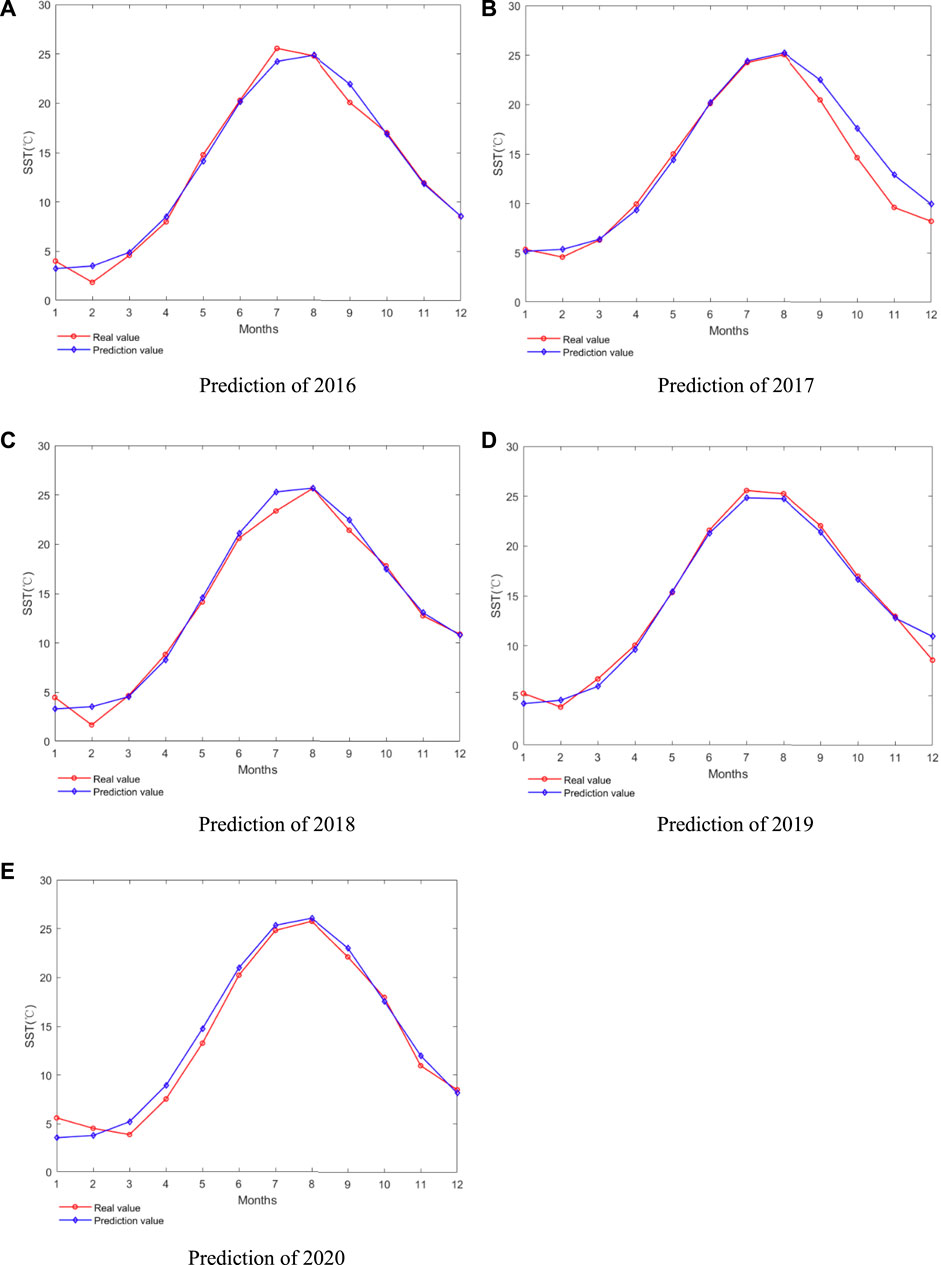
FIGURE 8. Consecutive prediction of the recent 5 years.
The overall prediction trend and real condition in recent 5 years are shown in Figure 9. The overall data trend of the two predictions is the same, and the MRE of all of the respective prediction is larger. The MRE of the prediction value is 9.84%. Using the same method to predict from 2016 to 2019, the MRE is 11.84%, 8.52%, 13.28%, and 5.54%. Compared with the real value, the prediction value obtained using this method in the continuous prediction of the past 5 years has a maximum MRE of 13.91%, a minimum of 7.80%, and an average of 11.07%. The average values of RMSE, LCCC, and RPD are 1.0603, 0.9894, and 7.497, respectively. The average monthly SST from 1985 to 2020 is selected to predict the SST in the next 50 years, and the obtained results are given in Figure 10. It also predicted the daily average SST in each month.
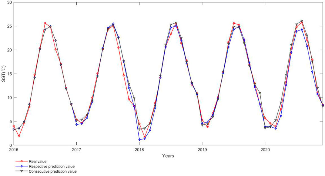
FIGURE 9. Respective prediction vs. consecutive prediction.
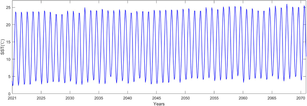
FIGURE 10. Change trend of SST from 2021 to 2070.
Due to the limitation of time and data, there are still more work conducted in future study. For example,
(1) In the process of predicting sea surface temperature, only the temperature itself is considered for analysis and prediction. Actually, SST is related to a set of factors such as atmospheric temperature, sea water salinity, ocean current movement, and so on. These factors should be considered comprehensively in the model, and the factors should be weighted to rank the influencing factors to find out the physical theories that really affect the SST.
(2) Because the effective time interval of time series prediction is short, the longer the prediction time is, the greater the error will be. In addition, since many countries have been aware of the impact of global warming, they will take more green and sustainable measures to mitigate the adverse trend in the future. Therefore, the prediction results of this study after 50 years are believed to have certain deviation from the measured results.
(3) We used the cubic spline interpolation method to fill the null values, which will definitely cause deviation from the real value. In the selection of data points, only the data near the center of the Bohai Sea were collected, and the data from other areas were ignored. The model established on the data set may not be completely applicable universally.
In this study, based on the empirical prediction method, the grey prediction method is used to analyze the sea surface temperature changing trend and create the prediction model. The prediction models are validated by the mean relative error and the similarity deviation metrics. The main work and achievements of this study are summarized as follows:
(1) The study carried out the analysis by experience prediction methods, considering that the SST has certain periodicity and the sustainability of change, similarity, and correlation with other marine elements, to make a qualitative or quantitative prediction. The method is simple and easy to construct, the predict effect is satisfactory. The MRE of this model is 4.20% when describing the monthly average SST in 2020.
(2) According to the constructed grey prediction model, a validation experiment was conducted from January to December 2020. The experiment combined the similarity deviation in statistics, establishing a model by selecting appropriate similar years, and then predicting the target year. The MRE of the prediction value is 9.84%. Using the same method to predict from 2016 to 2019, the MRE values are 11.84%, 8.52%, 13.28%, and 5.54%. Compared with the real value, the prediction value obtained using this method in the continuous predict of the past 5 years has a maximum MRE of 13.91%, a minimum of 7.80%, and the average values of MRE RMSE, LCCC, and RPD are 11.07% 1.0603, 0.9894, and 7.497, respectively. It also predicted the daily average SST in each month of 2020. The MRE is between 1.49% and 9.89%. The lowest result appears in December and the highest occurs in March.
We appreciate the data provided by National Science and Technology Resource Sharing Service Platform - National Marine Science Data Center (http://mds.nmdis.org.cn/ accessed on 10 January 2021). Information about the data accessed can be found in the article, further inquiries can be directed to the corresponding authors.
Conceptualization: JG, FM, and XL; methodology, data curation, formal analysis, investigation, and writing—original draft preparation: FM, ZQ, MG, and JC; and writing—review andediting and supervision: JG, LW-e, and FM. All authors have read and agreed to the published version of the manuscript.
This research was funded by the National Natural Science Foundation of China, grant number 41671158, supported by the Foundation of Liaoning Educational Committee (LJKZ0979), supported by the College Students’ Innovative Entrepreneurial Training Plan Program (S202110165051), and supported by Youth Innovation Promotion Association of Chinese Academy of Sciences to LW-e.
The authors would like to thank Liaoning Normal University for the laboratory facilities and the necessary technical support. They also thank the National Science and Technology Resource Sharing Service Platform (China National Marine Science Data Center) for data support.
The authors declare that the research was conducted in the absence of any commercial or financial relationships that could be construed as a potential conflict of interest.
All claims expressed in this article are solely those of the authors and do not necessarily represent those of their affiliated organizations, or those of the publisher, the editors, and the reviewers. Any product that may be evaluated in this article, or claim that may be made by its manufacturer, is not guaranteed or endorsed by the publisher.
Cui, L., and Liu, S. (2012). Characteristics and application on GM(1,1) model based on sequence of random vibration. Math. Pract. Knowl. 42 (11), 160–165. 10.3969j.issn.1000-0984.2012.11.021
Dong, Z., Teng, J., and Wang, J. (2008). Application of phase space reconstruction and ANFIS model in SST forecasting. J. Trop. Oceanogr. 27 (4), 73–76. doi:10.3969/j.issn.1009-5470.2008.04.011
He, Q., Cheng, Z., Song, W., Qi, F., Hao, Z., and Huang, D. (2020). Sea surface temperature prediction algorithm based on STL model. Mar. Environ. Sci. 39 (6), 918–925. doi:10.13634/j.cnki.mes.2020.06.015
Jin, J., Ding, J., and Wei, Y. (1999). Application of threshold auto‐regressive model based on genetic algorithm in sea surface temperature prediction. Mar. Environ. Sci. Technol. 18 (3), 1–6. doi:10.3969/j.issn.1007-6336.1999.03.001
Kim, M., Yang, H., and Kim, J. (2020). sea surface temperature and high water temperature occurrence prediction using a long short-term memory model. Remote Sens. (Basel). 12, 3654. doi:10.3390/rs12213654
Li, W., Lei, G., Qu, L., and Guo, D. (2020). Prediction of sea surface temperature in the China seas based on long short-term memory neural networks. Remote Sens. (Basel). 12, 2697. doi:10.3390/rs12172697
Li, Z., and Liu, S. (2020). Oscillation sequence prediction based on the gray interval GM(1, 1) model: Taking Shanghai Consumer Confidence Index as an example. Statistics Decis. 36 (14), 145–148. doi:10.13546/j.cnki.tjyjc.2020.14.032
Lu, H., Xie, C., Zhang, C., and Zhai, J. (2021). CMIP5-Based projection of decadal and seasonal sea surface temperature variations in East China shelf seas. J. Mar. Sci. Eng. 9, 367. doi:10.3390/jmse9040367
Lu, X., Sun, Y., and Da, L. (2009). Prediction of seawater temperature time series based on EMD. Mar. Technol. 28 (3), 79–82. doi:10.3969/j.issn.1003-2029.2009.03.021
Qian, W., and Dang, Y. (2009). GM(1, 1) model based on oscillation sequence. Syst. Eng. Theory Pract. 29 (03), 149–154. doi:10.3321/j.issn:1000-6788.2009.03.021
Qu, P., Wang, W., Liu, Z., Gong, X., Shi, C., and Xu, B. (2021). Assessment of a fusion sea surface temperature product for numerical weather predictions in China: A case study. Atmosphere 12, 604. doi:10.3390/atmos12050604
Shen, Y., Zhang, L., Zhou, X. Q., Fang, Y. M., Liu, Y., and Ma, L. Q. (2016). Photosynthetic electron-transfer reactions in the gametophyte of Pteris multifida reveal the presence of allelopathic interference from the invasive plant species Bidens pilos. J. Photochem. Photobiol. B 43 (04), 81–88. doi:10.1016/j.jphotobiol.2016.02.026
Shi, W., Zhu, B., and Zhang, C. (2018). Analysis and prediction of China's Marine industrial structure based on grey model. J. Zhejiang Ocean Univ. Humanit. Ed. 35 (04), 1–8. doi:10.3969/j.issn.1008-8318.2018.04.001
Sun, D., Song, J., Ren, K., Li, X., and Wang, G. (2020). A survey on the relationship between ocean subsurface temperature and tropical cyclone over the western north pacific. Adv. Meteorology 2020, 1–14. doi:10.1155/2020/9290837
Sung, H. M., Kim, J., Lee, J.-H., Shim, S., Boo, K.-O., Ha, J.-C., et al. (2021). Future changes in the global and regional sea level rise and sea surface temperature based on CMIP6 models. Atmosphere 12, 90. doi:10.3390/atmos12010090
Tang, L., Jia, D., and Meng, Q. (2008). To accomplish gray forecasting GM(1,1) model using the MATLAB. J. Cangzhou Teach. Coll. 24 (02), 35–37. doi:10.3969/j.issn.1008-4762.2008.02.017
Wang, H., Song, T., Zhu, S., Yang, S., and Feng, L. (2021). Subsurface temperature estimation from sea surface data using neural network models in the western Pacific ocean. Mathematics 9, 852. doi:10.3390/math9080852
Wang, J. (2017). Study on the influence of high speed railway on regional economy in Beijing Tianjin Hebei region. Beijing: Capital University of Economics and Business. doi:10.7666/d.D01197223
Wang, J., and Luo, D. (2017). Fractional discrete GM(1, 1) power model of oscillating sequence and its application. Control Decis. 32 (01), 176–180. doi:10.13195/j.kzyjc.2015.1233
Wang, Y., Chen, P., and Chen, X. (2013). Characteristics of sea surface temperature for major ecosystems in the Northwest Pacific under climate change. J. Shanghai Ocean Univ. 38 (6), 1–14. doi:10.12024/jsou.20200603074
Wang, Z. (2013). Models derived GM(1,1) power model. Syst. Eng. Theory Pract. 33 (11), 2894–2902. doi:10.12011/1000-6788(2013)11-2894
Yin, P. (2017). Grey predicting system GM(1, 1) model and its realization in Matlab. Heilongjiang Water Conservancy Sci. Technol. 45 (07), 16–18. doi:10.3969/j.issn.1007-7596.2017.07.005
Zeng, B., and Li, H. (2021). Prediction of coalbed methane production in China based on an optimized grey system model. Energy fuels. 35 (5), 4333–4344. doi:10.1021/acs.energyfuels.0c04195
Zeng, B., Tong, M., and Ma, X. (2020). A new-structure grey Verhulst model: Development and performance comparison. Appl. Math. Model. 81, 522–537. doi:10.1016/j.apm.2020.01.014
Zeng, L. (2019). Grey GM(1,1|sin) power model based on oscillation sequences and its application. J. Zhejiang Univ. Sci. Ed. 46 (06), 697–704. doi:10.3785/j.issn.1008-9497.2019.06.010
Zhang, J. (2004). Lectures on sea temperature predicting knowledge. Ocean. Predict 21 (1), 85–90. doi:10.3969/j.issn.1003-0239.2004.01.013
Zhang, Y., Tan, Y., and Peng, F. (2019). Study on time series prediction model of sea surface temperature based on Ensemble Empirical Mode Decomposition and Autoregressive Integrated Moving Average. J. Mar. Sci. 37 (1), 9–14. doi:10.3969/j.issn.1001-909X.2019.01.002
Zhang, Z., Pan, X., Jiang, T., Sui, B., Liu, C., and Sun, W. (2020). Monthly and quarterly sea surface temperature prediction based on gated recurrent unit neural network. J. Mar. Sci. Eng. 8, 249. doi:10.3390/jmse8040249
Zhao, D., Arshad, M., Li, N., and Triantafilis, J. (2021b). Predicting soil physical and chemical properties using vis-NIR in Australian cotton areas. Catena 196, 104938. doi:10.1016/j.catena.2020.104938
Zhao, D., Arshad, M., Wang, J., and Triantafilis, J. (2021a). Soil exchangeable cations estimation using Vis-NIR spectroscopy in different depths: Effects of multiple calibration models and spiking. Comput. Electron. Agric 182, 105990. doi:10.1016/j.compag.2021.105990
Keywords: sea surface temperature, grey theory, GM(1,1|sin) power model, genetic algorithm, prediction
Citation: Meng F, Gu J, Wang L-e, Qin Z, Gao M, Chen J and Li X (2022) A quantitative model based on grey theory for sea surface temperature prediction. Front. Environ. Sci. 10:1014856. doi: 10.3389/fenvs.2022.1014856
Received: 09 August 2022; Accepted: 14 October 2022;
Published: 10 November 2022.
Edited by:
Bing Xue, Institute for Advanced Sustainability Studies (IASS), GermanyReviewed by:
Dongrui Han, Shandong Academy of Agricultural Sciences, ChinaCopyright © 2022 Meng, Gu, Wang, Qin, Gao, Chen and Li. This is an open-access article distributed under the terms of the Creative Commons Attribution License (CC BY). The use, distribution or reproduction in other forums is permitted, provided the original author(s) and the copyright owner(s) are credited and that the original publication in this journal is cited, in accordance with accepted academic practice. No use, distribution or reproduction is permitted which does not comply with these terms.
*Correspondence: Jilin Gu, Z3VqaWxpbkBsbm51LmVkdS5jbg==; Ling-en Wang, d2FuZ2xlQGlnc25yci5hYy5jbg==
Disclaimer: All claims expressed in this article are solely those of the authors and do not necessarily represent those of their affiliated organizations, or those of the publisher, the editors and the reviewers. Any product that may be evaluated in this article or claim that may be made by its manufacturer is not guaranteed or endorsed by the publisher.
Research integrity at Frontiers
Learn more about the work of our research integrity team to safeguard the quality of each article we publish.