TripleConvTransformer: A deep learning vessel trajectory prediction method fusing discretized meteorological data

The shipping industry is increasingly threatened by global climate change. Reliable trajectory prediction can be used to perceive potential risks and ensure navigation efficiency. However, many existing studies have not fully considered the impact of complex ocean environmental factors and have only focused on local regions, which are difficult to extend to a global scale. To this end, we propose a deep learning vessel trajectory prediction method fusing discretized meteorological data (TripleConvTransformer). First, we clean the automatic identification system data to form a high-quality spatiotemporal trajectory dataset. Then, we fuse the trajectory data with the meteorological data after feature discretization to deeply mine the motion information of ocean-going ships. Finally, we design three modules, the global convolution, local convolution, and trend convolution modules, based on the simplified transformer model to capture multiscale features. We compare TripleConvTransformer with state-of-the-art prediction models. The experimental results show that in the prediction of the trajectory points in the next 90 min, the smallest root mean square error in terms of longitude and latitude and the highest overall prediction accuracy are achieved using TripleConvTransformer. Our method not only fully considers the influence of meteorological factors in the ocean-going process but also effectively extracts the important information hidden in the data, thus achieving accurate trajectory prediction on a global scale.

1 Introduction

As the most important carrier of global trade, shipping is still the main method of global cargo transportation (United Nations Conference on Trade and Development, 2021). However, disasters caused by climate change, such as the rise in sea level, the increase in rainfall, and the formation of tropical storms, will lead to infrastructure damage and trade disruptions in the shipping industry, resulting in large economic loss (Koetse and Rietveld, 2009; Zuccaro and Leone, 2021; Bhatti et al., 2022a; Bhatti et al., 2022b). In addition, the total emissions from global shipping continue to grow (Capaldo et al., 1999; Wang et al., 2021). This shows that the shipping industry is contributing to global climate change and destroying the marine ecological environment, which will ultimately be detrimental to itself (Liu et al., 2016; Mudryk et al., 2021).

One-way ocean freight shipping takes an average of approximately 30 days (Hummels and Schaur, 2013). During long voyages, vessels inevitably encounter extremely bad weather conditions, traffic management in busy sea areas, and navigation yaw errors (Szlapczynski and Krata, 2018). In addition, the power output of the vessel is insensitive and it has the particularity of being carried by the fluid, which makes the response time for changing the course of the vessel longer (Kim et al., 2021). If correct decisions with respect to the vessel cannot be made in a timely manner, according to the current state in the ocean-going process, the risk of life and the loss of property will greatly increase (Zhao et al., 2019). According to the International Convention for the Safety of Life at Sea (SOLAS), an automatic identification system (AIS) is a mandatory fit in all cargo ships (over 300 gross tonnage) and passenger ships (Solas, 2003). The AIS has the characteristics of global coverage, great compatibility, and strong real-time performance, which can provide stable data support for ocean-going ships (Qian et al., 2021). The vessel trajectory is usually used to describe the state of ship navigation (Gan et al., 2018). Figure 1 shows the AIS trajectories of bulk carriers worldwide. Trajectory prediction attempts to estimate the vessel trajectory for a period of time in the future based on historical navigation data (Hexeberg et al., 2017). Reliable trajectory prediction can be used to perceive potential risks and ensure navigation efficiency, which eliminates existing safety hazards and reduces emissions (Tong et al., 2015). Therefore, research on vessel trajectory prediction is of great significance to the shipping industry and even the fields of climate change and ecology (Tai and Robinson, 2018; Wan et al., 2018; Desai et al., 2021; Glassmeier et al., 2021).

FIGURE 1

FIGURE 1. AIS trajectories of 7,849 bulk carriers in 2021.

In recent years, vessel trajectory prediction has become a research hotspot in the shipping industry (Xiao et al., 2020a). Some traditional methods use statistical theory to establish ship motion equations for trajectory prediction (Sutulo et al., 2002; Perera and Soares, 2010; Mazzarella et al., 2015; Borkowski, 2017). Sutulo et al. proposed a simplified but fast dynamic maneuvering model and two kinematic prediction methods (a prediction based on current values of velocities and accelerations and a method to anticipate the ship’s trajectory after a course changing maneuver) (Sutulo et al., 2002). High computational speed was achieved in this work by eliminating a number of secondary effects and an extremely small amount of necessary input data but sacrificed accuracy and failed to ensure the prediction accuracy in complex sea areas. Perera et al. used the extended Kalman filter incorporated with a curvilinear motion model and a linear measurement model to achieve satisfactory prediction of ocean vessel positions, velocities, and accelerations (Perera and Soares, 2010). However, this study assumed that the mean acceleration components are constant values with white Gaussian noise, which is difficult to adapt to real navigation with changing acceleration conditions. Mazzarella et al. proposed a Bayesian vessel prediction algorithm based on a particle filter (Mazzarella et al., 2015). This algorithm, aided by the knowledge of traffic routes, enhanced the quality of the vessel position prediction, but it also increased the computational complexity. Borkowski presented an algorithm of ship movement trajectory prediction (Borkowski, 2017). This algorithm made use of measurements of the ship’s current position from a number of doubled autonomous devices through navigational data fusion and took the assumption of knowledge of both future course alterations and the parameters of the ship dynamics model into account. However, the performance of this algorithm was dependent on high-quality data and reliable assumptions, which were not necessarily satisfied in complex sea areas.

Obviously, the traditional methods based on statistical theory have high computational complexity and rely on domain knowledge, making it difficult for them to establish effective prediction models in complex marine environments (Xiao et al., 2022b). In recent years, data-driven deep neural networks have gradually become the preferred schemes for trajectory prediction tasks due to their advantages of high computational efficiency and strong adaptability (Rong et al., 2019; Capobianco et al., 2021; Liu R. W. et al., 2022; Liu X. et al., 2022; Yang et al., 2022). Rong et al. proposed a probabilistic trajectory prediction model to describe the uncertainty in future positions along ship trajectories and a data-driven nonparametric Bayesian model based on a Gaussian process to describe the lateral motion uncertainty, thus achieving high prediction accuracy and meeting the demands of real-time applications (Rong et al., 2019). Capobianco et al. presented a recurrent encoder-decoder architecture that was able to learn space-time dependencies from historical ship mobility data to address the problem of trajectory prediction in the presence of complex mobility patterns (Capobianco et al., 2021). Liu et al. used the data-driven predictor developed with a long short-term memory (LSTM) network to calculate the trajectory and uncertainty for the future moment and achieved uncertainty fusion by fusing the output of the data-driven predictor with the vessel motion estimation, thus making the predicted trajectory sequence more accurate (Liu X. et al., 2022). Yang et al. proposed a vessel trajectory prediction method that combined data denoising and a bidirectional long short-term memory (Bi-LSTM) model to achieve accurate short-term prediction of the trajectory sequence (Yang et al., 2022). Liu et al. proposed a spatiotemporal multigraph convolutional network (STMGCN)-based trajectory prediction framework and designed a self-attention temporal convolution layer to optimize the STMGCN, thus achieving superior prediction performance in terms of both accuracy and robustness (Liu R. W. et al., 2022).

At present, trajectory prediction methods based on deep learning technology have achieved promising results. However, many existing studies have not fully considered the impact of complex ocean environmental factors. It is well known that adverse weather conditions (such as fog, lack of light, rain and snow) In addition to the seawater density, the seawater temperature, sea wind, and sea waves have an impact on the motion behaviors of ships (Szlapczynski and Krata, 2018). Therefore, incorporating these factors into the model can ensure more satisfactory prediction results. In addition, the current studies only conduct an experimental analysis of vessel trajectory prediction in local sea areas such as canals and ports. Ship navigation in a canal area is one-way, and the ship channel is constrained by the river (Elsherbiny et al., 2020). Ships entering and leaving the port must follow the guidance of the pilots and the regulations of the specific channel (Liu et al., 2010). In these local sea areas, the ship motion is greatly restricted, and the change in the air-sea environment is not obvious. The characteristics of these local sea areas make it difficult for the current studies to be extended to pelagic areas with greater freedom of navigation and a more complex environment.

To this end, we propose a deep learning vessel trajectory prediction method fusing discretized meteorological data (TripleConvTransformer). First, we clean the AIS data to form a high-quality spatiotemporal trajectory dataset. Then, we use the discretization method based on the minimum description length principle (MDLP) (Chen et al., 2021) to discretize the meteorological data and fuse the trajectory data with the meteorological data after feature discretization to deeply mine the motion information of ocean-going ships. Finally, we design three modules, the global convolution, local convolution, and trend convolution modules, based on the simplified transformer model (Vaswani et al., 2017) to capture multiscale features. We compare TripleConvTransformer with state-of-the-art prediction models on ship trajectory data in global sea areas. In the prediction of the trajectory points in the next 90 min, the smallest root mean square error in terms of longitude and latitude and the highest overall prediction accuracy are achieved using TripleConvTransformer. Experimental results verify the effectiveness of the proposed method.

The remainder of this paper is organized as follows. In Section 2, the related work is reviewed. In Section 3, the proposed vessel trajectory prediction model is elaborate. The experimental results are presented in Section 4. In Section 5, this paper is summarized, and potential future explorations are highlighted.

2 Related work

We introduce the three types of outliers that often appear in AIS data. Then, we illustrate the definition and the basic flow of feature discretization. Finally, we briefly review the deep learning models for time series forecasting.

2.1 Outliers in AIS

The AIS can provide important static and dynamic information, such as the ship’s Maritime Mobile Service Identity (MMSI), sampling point position, Speed Over Ground (SOG), and Course Over Ground (COG). However, due to the lack of a good information verification mechanism, the actual AIS data contain a large number of outliers (Liu X. et al., 2022). These outliers are mainly classified into abnormal drift points, abnormal stopping points, and abnormal numerical points, which are described as follows.

1) Abnormal drift point: The moving distance of the object in a given time is greater than the product of this object’s maximum speed and this time’s length.

2) Abnormal stopping point: The relevant information of the object is not in real time, or the object has the same information except for the time information.

3) Abnormal numerical point: There are illegal object values.

In addition, due to the large individual differences of ships, the manifestations of abnormal trajectory points are different. These data quality problems cause great resistance to AIS-based trajectory prediction.

2.2 Feature discretization

Feature discretization is an important data preprocessing technology in big data analysis (Chen et al., 2022a). In feature discretization, continuous attributes are divided into a finite number of subintervals, and then, these subintervals are associated with a set of discrete values (Chen and Huang, 2022). Feature discretization can be used to remove redundant information and filter noise, thereby improving the generalization ability of the learning model (Chen et al., 2022b). In addition, feature discretization can be useful for missing value imputation (Rahman and Islam, 2016).

The basic flow of feature discretization is shown in Figure 2. First, the continuous attribute values are sorted, and the duplicate values are removed to obtain a set of candidate breakpoints. Second, the breakpoints of continuous attributes are selected from the set of candidate breakpoints, and whether to segment the interval or merge the adjacent subintervals is decided according to the judgment criteria of the adopted discretization algorithm. If the termination condition is satisfied, the discretization result is output; otherwise, the remaining breakpoints are continuously selected from the set of candidate breakpoints to perform attribute discretization.

FIGURE 2

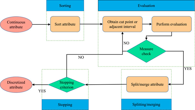
FIGURE 2. The basic flow of feature discretization.

2.3 Deep learning model for time series forecasting

Time series data widely exist in the fields of meteorology, transportation, finance, medical care, and the internet (Cook et al., 2020; Hasnain et al., 2022). Time series forecasting refers to the prediction of states in several future periods by analyzing changes in time series data. Owing to their high-dimensional, dynamic, and large-scale characteristics, it is extremely difficult to analyze time series data (Makridakis et al., 2018; Zhu et al., 2021). Compared with statistical models, deep learning models can more effectively mine historical information (Lim and Zohren, 2021). The informer model proposed by Zhou et al. drastically improved the inference speed of long-sequence predictions (Zhou et al., 2021). The SCINet model proposed by Liu et al. facilitated the extraction of temporal relation features (Liu et al., 2021).

At present, transformer models have excellent results in natural language processing, computer vision and time series forecasting. Transformer models do not utilize the recursive approach of recurrent neural networks; however, they have excellent structural advantages in modeling sequential problems. The main advantages for transformer models in time series prediction tasks are as follows: 1) They rely on a multiheaded self-attention mechanism that can maintain the ability to model both short-term and long-term time series features. 2) They support parallel computing, and model training is accelerated (Vaswani et al., 2017). These advantages allow complex problems to be modeled with excellent performance.

3 Improved transformer model for vessel trajectory prediction

We introduce the process of trajectory extraction and meteorological data discretization in detail. Then, we design the model framework and explain the three convolution modules and the self-attention mechanism. Finally, we elaborate the overall flow of the proposed algorithm.

3.1 Trajectory extraction

We use a five-dimensional vector $S\left(T,X,Y,V,C\right)$ containing time, longitude, latitude, SOG, and COG to describe the real-time state of a vessel. A complete vessel trajectory T consists of multiple trajectory points, which can be expressed as $T={\{S}_1,S_2,S_3,\dots ,S_i\}$. The state S of each trajectory point is obtained from the AIS data. Since there is no good information verification mechanism, the AIS data contain a large number of abnormal drift points, abnormal stopping points, and abnormal numerical points. We identify and address these outliers as follows.

1) Abnormal drift points: The longitude and latitude information of AIS often deviates significantly in a short period, as shown in Figure 3. If the linear distance $d\left(i,i+\mathit{1}\right)$ between the trajectory points $i$ and $i+\mathit{1}$ of two consecutive moments satisfies the following expression:

$\mathit{d}\left(\mathit{i},\mathit{i}+\mathbf{1}\right)>{\mathit{V}}_{\mathit{max}}\times ∆\mathit{T},(1)$

FIGURE 3

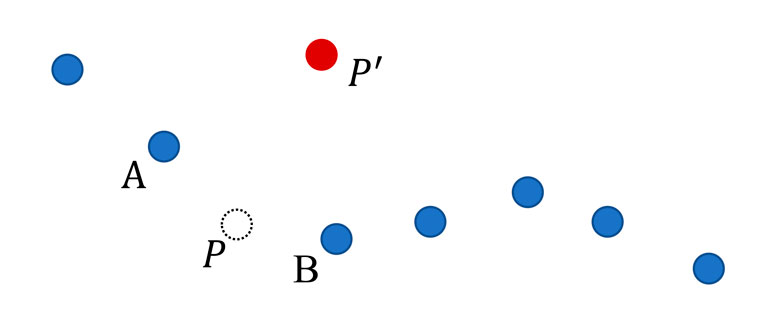
FIGURE 3. Scenario where abnormal drift points appear in the AIS. ${\mathit{P}}^{\prime }$ is an abnormal drift point; A and B are the two trajectory points before and after the point adjacent to ${\mathit{P}}^{\prime }$ in the trajectory sequence, respectively; P is the position point where ${\mathit{P}}^{\prime }$ should have existed under normal circumstances.

then the trajectory point $i+\mathit{1}$ is regarded as an abnormal drift point. $V_{\mathit{max}}$ is the maximum speed for which the vessel is designed. $∆T$ is the time interval between trajectory points $i$ and $i+\mathit{1}$. $d\left(i,i+\mathit{1}\right)$ can be calculated by the Haversine formula:

$\begin{array}{c}\mathit{d}\left(\mathit{i},\mathit{i}+\mathrm{1}\right)=\mathrm{2}\mathit{r}{\mathit{sin}}^{-\mathrm{1}}\left(\sqrt{{\mathit{sin}}^{\mathrm{2}}\left(\frac{{\mathit{\phi }}_{\mathrm{2}}-{\mathit{\phi }}_{\mathrm{1}}}{\mathrm{2}}\right)+\mathit{cos}\left({\mathit{\phi }}_{\mathrm{1}}\right)\mathit{cos}\left({\mathit{\phi }}_{\mathrm{2}}\right){\mathit{sin}}^{\mathrm{2}}\left(\frac{{\mathit{\lambda }}_{\mathrm{2}}-{\mathit{\lambda }}_{\mathrm{1}}}{\mathrm{2}}\right)}\right),\end{array}(2)$

where $r$ is the radius of the earth. ${\lambda }_{\mathit{1}}$ and ${\lambda }_{\mathit{2}}$ represent the longitudes of trajectory points $i$ and $i+\mathit{1}$, respectively. ${\phi }_{\mathit{1}}$ and ${\phi }_{\mathit{2}}$represent the latitudes of the trajectory points $i$and $i+\mathit{1}$, respectively.

2) Abnormal stopping points: The AIS data forwarding mechanism usually makes the receiver receive multiple duplicate records at the same trajectory point. In addition, the ship positioning equipment cannot obtain the current position information in real time under some complex air-sea conditions, resulting in repeated information of successive positions. If $\left(X,Y,V,C\right)$ of the $i$-th trajectory point’s state $S_i$is the same as that of the $i+\mathit{1}$-th trajectory point’s state $S_{i+\mathit{1}}$, then the $i+\mathit{1}$-th trajectory point can be regarded as an abnormal stopping point.

3) Abnormal numerical point: The effect of environmental conditions and interference in the transmission channel inevitably result in abnormal AIS equipment data, which are also affected by the quality of sensors. AIS specifications and ship parameters are described in Table 1. We use this information as the criterion for outlier judgment.

TABLE 1

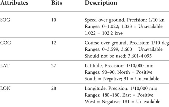
TABLE 1. Description of important AIS attributes.

The research objects of this paper are mainly large ocean-going bulk carriers with a deadweight of over 20,000 tons. These large vessels have high motion inertia and slow speed and are more stable than other ships during normal navigation. Thus, we treat the extreme distribution values as outliers. We take the SOG numerical distribution shown in Figure 4 as an example to illustrate the process of outlier judgment. From the SOG numerical distribution, it can be seen that the vessel will rarely exceed the designed service speed of the ship in the process of normal navigation, and the speed distribution is concentrated. Thus, we regard speed over the ground values of less than 5 kn and more than 25 kn as outliers.

FIGURE 4

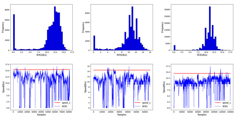
FIGURE 4. SOG numerical distribution. The upper three subgraphs are the SOG numerical distribution histograms. The lower three subgraphs are the SOG numerical line charts, in which the red horizontal line is the designed service speed of the ship.

After the outliers are processed, a relatively reliable dataset of ocean-going vessel trajectories can be obtained. Then, we segment the trajectory data of all vessels to form consecutive subtrajectories with controllable time intervals that are suitable for trajectory prediction modeling. According to the requirements of the AIS, the maximum time interval for the ship to report outward under the anchoring state is 3 min. Thus, when the reporting interval exceeds 3 min, the data are not referential. Figure 5 shows the distribution of trajectory data. The length of subtrajectories formed after trajectory segmentation is not fixed. Since subtrajectories with extremely short lengths are not suitable for modeling by deep learning, we stipulate that only subtrajectories containing at least 120 points can be retained.

FIGURE 5

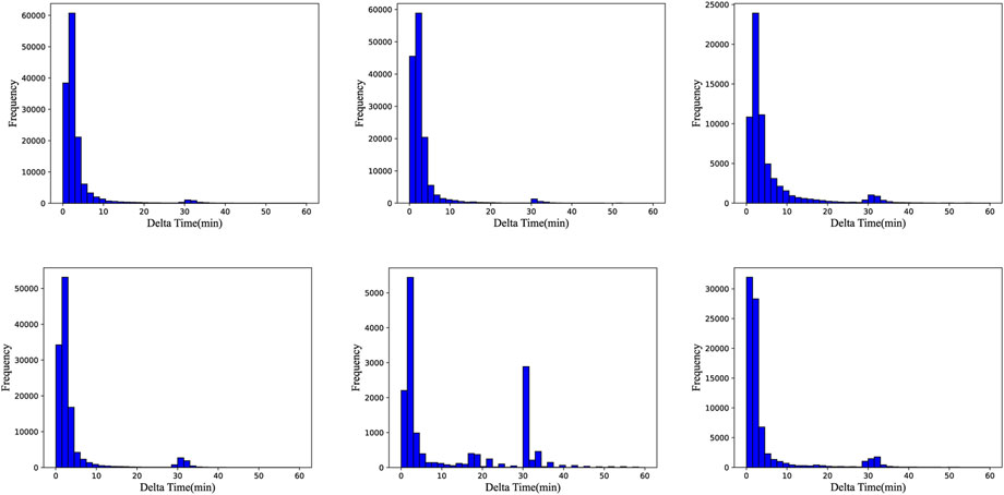
FIGURE 5. Trajectory data distribution. The abscissa indicates the time interval between two adjacent trajectory points on the trajectory sequence; the ordinate indicates the frequency of occurrence.

3.2 Meteorological data discretization

Meteorological conditions are an important factor to be considered in the process of ship navigation. However, there is usually considerable redundant information, noise, and even missing values in the collected meteorological data. To effectively fuse the meteorological data and AIS data, we perform feature discretization on the meteorological data. First, we use the k-means algorithm to cluster the unlabeled meteorological data. Compared with other clustering algorithms (McInnes and Healy, 2017), the k-means algorithm has low time complexity and high efficiency on large-scale datasets. However, the value of k plays a decisive role in the clustering effect. To obtain the best clustering effect, we choose the gap statistics method to determine the value of k (Tibshirani et al., 2001). Then, we use a discretization method based on MDLP for feature discretization of meteorological data. The discretization method based on MDLP evaluates the discretization results by information gain.

Suppose that the meteorological dataset $S$ contains $k$ categories $C_1$, …, $C_k$, and $P\left(C_i,S\right)$ represents the occurrence frequency of category $C_i$ in $S$; then, the information entropy of $S$ is defined as (Fayyad and Irani, 1993):

$\begin{array}{c}\mathit{E}\mathit{n}\mathit{t}\left(\mathit{S}\right)=-{\displaystyle \sum }_{\mathit{i}=\mathrm{1}}^{\mathit{k}}\mathit{P}\left({\mathit{C}}_{\mathit{i}},\mathit{S}\right)\mathit{log}\left(\mathit{P}\left({\mathit{C}}_{\mathit{i}},\mathit{S}\right)\right)\end{array}(3)$

Suppose that $S$ is divided into two subsets $S_{\mathit{1}}$ and $S_{\mathit{2}}$ by breakpoint $T$; then, the breakpoint information entropy of $S$ is defined as follows:

$\mathit{E}\left(\mathit{A},\mathit{T},\mathit{S}\right)=\frac{\left|{\mathit{S}}_{\mathrm{1}}\right|}{\left|\mathit{S}\right|}\mathit{E}\mathit{n}\mathit{t}\left({\mathit{S}}_{\mathrm{1}}\right)+\frac{\left|{\mathit{S}}_{\mathrm{2}}\right|}{\left|\mathit{S}\right|}\mathit{E}\mathit{n}\mathit{t}\left({\mathit{S}}_{\mathrm{2}}\right),(4)$

where $\left|S\right|$, $\left|S_1\right|$, and $\left|S_2\right|$ are the number of samples contained in $S$, $S_{\mathit{1}}$, and $S_{\mathit{2}}$, respectively, and $A$ is the meteorological attribute to be discretized. The breakpoint $T_A$ that minimizes $Ent\left(A,T,S\right)$ is the optimal breakpoint, which is selected to perform binary discretization of $A$. The information gain of $S$ after discretization is:

$\mathit{G}\mathit{a}\mathit{i}\mathit{n}\mathit{s}\left(\mathit{A},{\mathit{T}}_{\mathit{A}},\mathit{S}\right)=\mathit{E}\mathit{n}\mathit{t}\left(\mathit{S}\right)-\mathit{E}\mathit{n}\mathit{t}\left(\mathit{A},{\mathit{T}}_{\mathit{A}},\mathit{S}\right).(5)$

In addition, the selected breakpoint needs to meet the following conditions:

$\mathit{G}\mathit{a}\mathit{i}\mathit{n}\mathit{s}\left(\mathit{A},{\mathit{T}}_{\mathit{A}},\mathit{S}\right)>\frac{{\mathit{log}}_{\mathrm{2}}\left(\mathit{N}-\mathrm{1}\right)}{\mathit{N}}+\frac{∆\left(\mathit{A},{\mathit{T}}_{\mathit{A}},\mathit{S}\right)}{\mathit{N}},(6)$

$∆\left(\mathit{A},{\mathit{T}}_{\mathit{A}},\mathit{S}\right)={\mathit{log}}_{\mathrm{2}}\left({\mathrm{3}}^{\mathit{k}}-\mathrm{2}\right)-\left[\mathit{k}\mathit{E}\mathit{n}\mathit{t}\left(\mathit{S}\right)-{\mathit{k}}_{\mathrm{1}}\mathit{E}\mathit{n}\mathit{t}\left({\mathit{S}}_{\mathit{1}}\right)-{\mathit{k}}_{\mathrm{2}}\mathit{E}\mathit{n}\mathit{t}\left({\mathit{S}}_{\mathit{2}}\right)\right],(7)$

where $N$ is the total number of samples in the meteorological dataset and $k_{\mathit{1}}$ and $k_{\mathit{2}}$ are the number of categories included in $S_{\mathit{1}}$ and $S_{\mathit{2}}$ (${k=k}_{\mathit{1}}+k_{\mathit{2}}$), respectively. The discretization method based on MDLP selects the optimal breakpoint that meets the above conditions in each iteration to divide the meteorological attributes, thus obtaining the optimal discretization results of meteorological data.

3.3 Model frame

To effectively mine the hidden features of ship motion from historical trajectory information and meteorological information, we design a network model (TripleConvTransformer) combining a convolutional neural network and a multihead attention mechanism. The network structure of TripleConvTransformer is shown in Figure 6. We use three different types of convolution modules to extract multiscale features.

1) Global Convolution: There are some fixed patterns during ship navigation. These patterns can well reflect the basic situation of vessels. We create a convolution layer with a convolution kernel matched to the input stride to extract the fixed patterns of each variable sequence in all time steps. The global convolution kernel size in this study is $\mathit{60}\times \mathit{1}$.

2) Local Convolution: Ship navigation is a consecutive motion process. Compared with the time steps farther from the current moment, the time steps closer to the current moment have greater internal correlation about the current moment. Local convolution focuses on extracting local contextual contacts. The size of the convolution kernel is the length of the local consecutive content. The local convolution kernel size in this study is $\mathit{5}\times \mathit{1}$.

3) Trend Convolution: The trajectory sequence is a time series with significant trends. We ensure the stability of the prediction results by fitting trends. Trends can be expressed by a polynomial function (Oreshkin et al., 2019). We use a convolution kernel with a size of $\mathit{1}\times \mathit{1}$ for feature extraction. Then, we multiply the convolution result set $\theta$ with the time matrix as follows:

$\widehat{\mathit{y}}={\displaystyle \sum }_{\mathit{i}=\mathit{0}}^{\mathit{p}}\mathit{\theta }{\mathit{t}}^{\mathit{i}}(8)$

where $\widehat{\mathit{y}}$ is the final output of the module, $t=\left[\mathit{0,1,2},\dots ,l-\mathit{2},l-\mathit{1}\right]/l$, $l$is the number of prediction time steps, and $p$ is the degree of the polynomial. When $p$ takes a small value such as 2 or 3, the model is able to imitate trends by learning $\theta$. In the experiments in this paper, we have chosen 3 for the value of $p$.

FIGURE 6

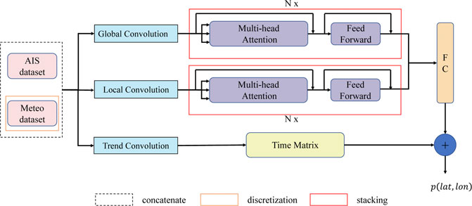
FIGURE 6. Network structure of TripleConvTransformer.

The self-attention mechanism has the advantages of parallel computing and a global receptive field (Vaswani et al., 2017). To this end, we add a multihead self-attention mechanism to the model to obtain the dependency between the features output by the convolution modules. The formula to calculate the dot product multihead attention is:

$\mathit{A}\mathit{t}\mathit{t}\mathit{e}\mathit{n}\mathit{t}\mathit{i}\mathit{o}\mathit{n}\left(\mathit{Q},\mathit{K},\mathit{V}\right)=\mathit{s}\mathit{o}\mathit{f}\mathit{t}\mathit{m}\mathit{a}\mathit{x}\left(\frac{\mathit{Q}{\mathit{K}}^{\mathit{T}}}{\sqrt{{\mathit{d}}_{\mathit{k}}}}\right)\mathit{V}(9)$

where $Q$, $K$, and $V$ are the query vector, key vector, and value vector, respectively, $d_k$ is the dimension of $K$, and the input is the feature set output by the convolution modules. TripleConvTransformer can directly obtain the relationship between any extracted features without being affected by the sequence order.

The overall flow of the proposed algorithm is shown in Figure 7. Our algorithm mainly includes three modules, namely, the AIS trajectory data extraction module, meteorological data feature discretization module, and deep learning module combining a convolutional neural network and multihead attention mechanism. First, we clean AIS data to form a high-quality spatiotemporal trajectory dataset. Then, we use the discretization method based on MDLP to perform feature discretization on the meteorological data and fuse the trajectory data with the meteorological data after feature discretization to deeply mine the motion information of ocean-going ships. Finally, we design three different types of convolution modules based on the simplified transformer model to capture multiscale features.

FIGURE 7

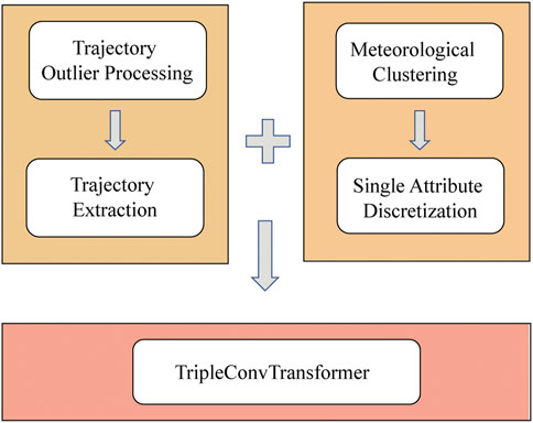
FIGURE 7. The overall flow of the proposed algorithm.

4 Experiments

We introduce the dataset and the experimental environment configuration. Then, we explain the three evaluation indicators for vessel trajectory prediction. Finally, we compare the proposed algorithm with state-of-the-art prediction models and present the experimental results.

4.1 Dataset

We use the AIS trajectory data of 7,849 bulk carriers with a deadweight over 20,000 tons in the whole year of 2021 and the meteorological data corresponding to the trajectory points to conduct experiments. After extracting the trajectories, we obtain 336,573 subtrajectories that meet the requirements. We take the top 70% subtrajectories of each vessel, a total of 109,564,853 trajectory points, as the training set. In the remaining subtrajectories of each vessel, the first 20% of the subtrajectories are used as the verification set, and the last 10% of the subtrajectories are used as the test set. The attributes contained in AIS data and meteorological data used in this experiment are listed in Table 2.

TABLE 2

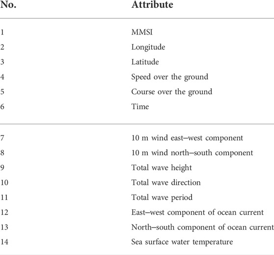
TABLE 2. The attributes contained in AIS data and meteorological data.

4.2 Experimental environment

The hardware environment of this experiment is a server with an Intel(R) Xeon(R) Gold 6248R CPU@3.00 GHz processor, 256 GB memory, and an NVIDIA RTX 3090 * 4 GPU. This experiment uses Python 3.7 and PyTorch 1.7 on the CentOS Linux release 7.6.1810 system for network simulation and testing.

4.3 Evaluation indicators

We use the three indicators of mean absolute error (MAE), root mean square error (RMSE), and goodness of fit ($R^2$) to evaluate the prediction ability of the model. The more MAE and RMSE tend to 0 and $R^2$ tends to 1, the higher the prediction accuracy. These three indicators are shown as follows:

$\mathit{M}\mathit{A}\mathit{E}=\frac{\mathrm{1}}{\mathit{n}}{\displaystyle \sum }_{\mathit{i}=\mathit{1}}^{\mathit{n}}\left|{\mathit{y}}_{\mathit{i}}-{\widehat{\mathit{y}}}_{\mathit{i}}\right|(10)$

$\mathit{R}\mathit{M}\mathit{S}\mathit{E}=\sqrt{\frac{\mathrm{1}}{\mathit{n}}{\displaystyle \sum }_{\mathit{i}=\mathrm{1}}^{\mathit{n}}{\left({\mathit{y}}_{\mathit{i}}-{\widehat{\mathit{y}}}_{\mathit{i}}\right)}^{\mathrm{2}}}(11)$

${\mathit{R}}^{\mathrm{2}}=\mathrm{1}-\frac{{\displaystyle \sum }_{\mathit{i}=\mathrm{1}}^{\mathit{n}}{\left({\widehat{\mathit{y}}}_{\mathit{i}}-{\mathit{y}}_{\mathit{i}}\right)}^{\mathrm{2}}}{{\displaystyle \sum }_{\mathit{i}=\mathrm{1}}^{\mathit{n}}{\left(\overline{\mathit{y}}-{\mathit{y}}_{\mathit{i}}\right)}^{\mathrm{2}}}(12)$

where $y_i$ is the true value, ${\widehat{y}}_i$ is the predicted value, $\overline{y}$ is the mean of all true values in the test set, and $n$ is the total number of samples. The data were normalized by the Z score method before being fed into the model for calculation. To more directly express the error, we denormalize it. The formula of denormalization is:

$\mathit{y}=\mathit{\sigma }\times \widehat{\mathit{y}}+\mathit{\mu }(13)$

where $\sigma$ is the standard deviation of all samples in the training set, and $\mu$ is the mean of all samples in the training set.

4.4 Experimental results

In the process of clustering meteorological data, we obtained a k value of 21 by the gap statistics method, as shown in Figure 8. Then, we perform feature discretization on meteorological data using a discretization method based on MDLP. The number of discrete intervals of meteorological attributes is shown in Table 3.

FIGURE 8

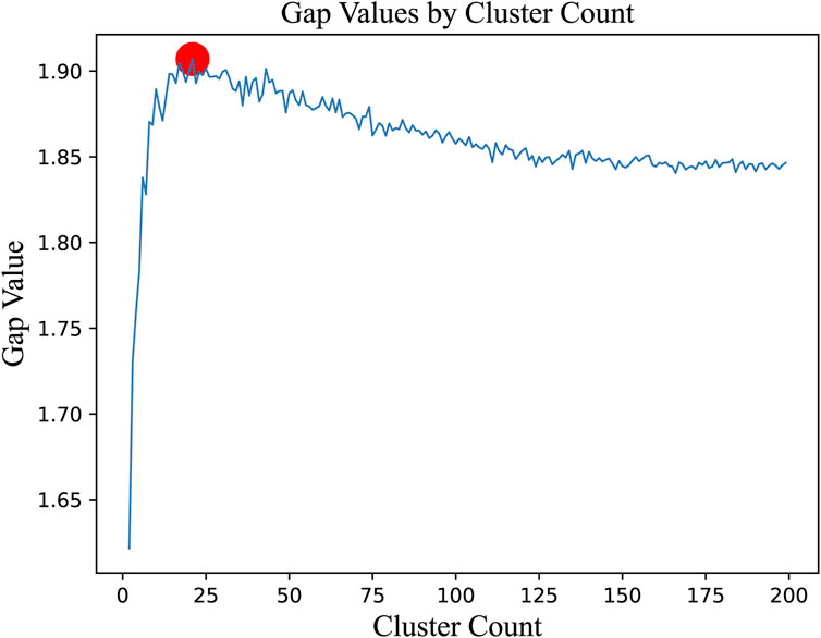
FIGURE 8. Variation curve of the gap value with respect to the cluster count. The red dot is the optimal number of clusters.

TABLE 3

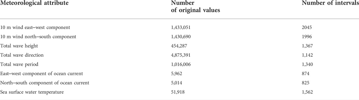
TABLE 3. The number of discrete intervals of meteorological attributes.

We verified the effectiveness of the designed combination of the three convolutional modules, and the experimental results are shown in Table 4. Bold content indicates the optimal results. The experimental results show that when global convolution, local convolution and trend convolution are combined into TripleConvTransformer, each metric has a significant advantage over any other combination. This proves that the three convolutional modules we designed accomplish the expected functions and are able to obtain optimal results in ship trajectory prediction.

TABLE 4

TABLE 4. Experimental results on the effectiveness of the three convolutional modules.

We compared TripleConvTransformer with the gate recurrent unit (GRU) (Cho et al., 2014), temporal convolutional network (TCN) (Bai et al., 2018), SCINet (Liu et al., 2021), and transformer (Vaswani et al., 2017) to evaluate the prediction accuracy of the proposed method. Table 5 shows the prediction results of the five algorithms in terms of longitude and latitude. The bolded values indicate the best results.

TABLE 5

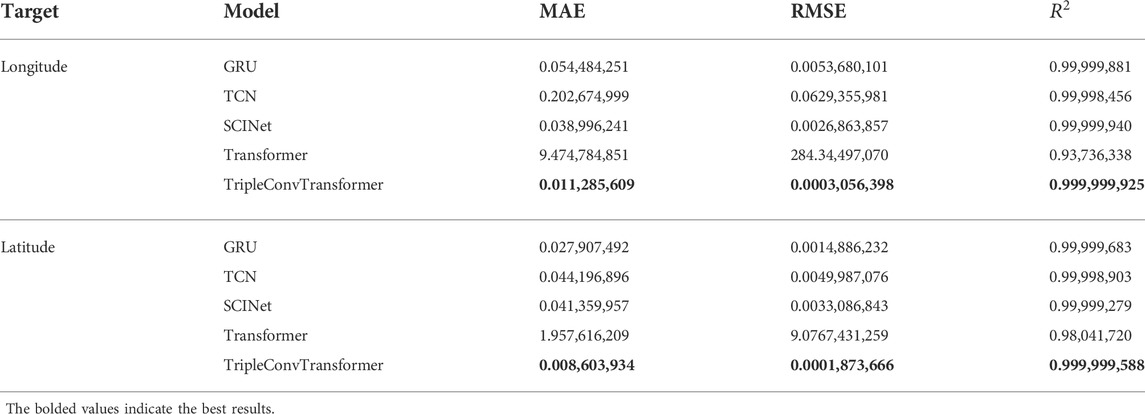
TABLE 5. Prediction results of the five algorithms on longitude and latitude.

TripleConvTransformer achieved the best metric values for all algorithms in terms of latitude and longitude forecasting. Additionally, we found that the transformer model, which was not optimized, performed poorly in the application of trajectory prediction. This is because the structure of the self-attention mechanism determines its lack of ability to record sequence position information. This means that the position encoding design has a very important impact on the results of the model. However, initial position encoding is a simple structure that does not perform well in the trajectory prediction task. In addition, the transformer model cannot pay special attention to the vessel navigation process characteristics mentioned in Section 3.3, which are included in the local convolution design. TripleConvTransformer can extract features in all dimensions and has some superiority in the network structure. The experimental results also show that TripleConvTransformer outperforms the other four algorithms in trajectory prediction in general.

5 Conclusion

Reliable trajectory prediction can be used to perceive potential risks and ensure navigation efficiency, which eliminates existing safety hazards and reduces emissions. In this paper, we have proposed a deep learning vessel trajectory prediction method fusing discretized meteorological data (TripleConvTransformer). Our contributions mainly come from the following aspects: 1) we have cleaned the AIS data to form a high-quality spatiotemporal trajectory dataset; 2) we have fused the trajectory data with the meteorological data after feature discretization to deeply mine the motion information of ocean-going ships; and 3) we have designed three modules, namely, the global convolution, local convolution, and trend convolution modules, based on the simplified transformer model to capture multiscale features. We compare TripleConvTransformer with the state-of-the-art prediction models. TripleConvTransformer achieves the best metric values among all models in terms of latitude and longitude forecasting. Although TripleConvTransformer has achieved exciting trajectory prediction results, the current model does not have a confidence index. If our algorithm can provide a confidence index to the captain, then the captain can better understand the reliability of the position information provided by the algorithm. This would be a large improvement with respect to the safe navigation of the vessel. In future research work, we will continue to improve the TripleConvTransformer model to achieve more accurate trajectory prediction results.

Data availability statement

The raw data supporting the conclusions of this article will be made available by the authors, without undue reservation.

Author contributions

PH and QC contributed equally to method design, experimental analysis, and manuscript writing. DW and MW contributed to the visualization. XW and XH were responsible for data provision and funding acquisition. All authors reviewed the final version of the manuscript and consented to publication.

Funding

This work was supported in part by the National Key Research and Development Program of China under Grant 2021YFC3101600, 2020YFA0607900, 2020YFA0608001, and 2020YFA0608003, in part by the Open Foundation of Key Laboratory of Marine Science and Numerical Modeling under Grant 2020-ZD-05, in part by the National Science Foundation of China under Grant 42075142, 42125503, and 42075137, in part by the Sichuan Science and Technology Program under Grant 2020JDTD0020 and 2019ZDZX0007, and in part by the China Postdoctoral Science Foundation under Grant 2021M701838.

Conflict of interest

The authors declare that the research was conducted in the absence of any commercial or financial relationships that could be construed as a potential conflict of interest.

Publisher’s note

All claims expressed in this article are solely those of the authors and do not necessarily represent those of their affiliated organizations, or those of the publisher, the editors and the reviewers. Any product that may be evaluated in this article, or claim that may be made by its manufacturer, is not guaranteed or endorsed by the publisher.

References

Bai, S., Kolter, J. Z., and Koltun, V. (2018). An empirical evaluation of generic convolutional and recurrent networks for sequence modeling. arXiv [Preprint]. Available at: https://arxiv.org/abs/1905.10437.

Google Scholar

Bhatti, U. A., Nizamani, M. M., and Mengxing, H. (2022a). Climate change threatens Pakistan’s snow leopards. Science 377 (6606), 585–586. doi:10.1126/science.add9065

PubMed Abstract | CrossRef Full Text | Google Scholar

Bhatti, U. A., Zeeshan, Z., Nizamani, M. M., Bazai, S., Yu, Z., and Yuan, L. (2022b). Assessing the change of ambient air quality patterns in Jiangsu Province of China pre-to post-COVID-19. Chemosphere 288, 132569. doi:10.1016/j.chemosphere.2021.132569

PubMed Abstract | CrossRef Full Text | Google Scholar

Borkowski, P. (2017). The ship movement trajectory prediction algorithm using navigational data fusion. Sensors 17 (6), 1432. doi:10.3390/s17061432

PubMed Abstract | CrossRef Full Text | Google Scholar

Capaldo, K., Corbett, J. J., Kasibhatla, P., Fischbeck, P., and Pandis, S. N. (1999). Effects of ship emissions on sulphur cycling and radiative climate forcing over the ocean. Nature 400 (6746), 743–746. doi:10.1038/23438

CrossRef Full Text | Google Scholar

Capobianco, S., Millefiori, L. M., Forti, N., Braca, P., and Willett, P. (2021). Deep learning methods for vessel trajectory prediction based on recurrent neural networks. IEEE Trans. Aerosp. Electron. Syst. 57 (6), 4329–4346. doi:10.1109/taes.2021.3096873

CrossRef Full Text | Google Scholar

Chen, Q., Ding, W., Huang, X., and Wang, H. (2022b). “Generalized interval type II fuzzy rough model based feature discretization for mixed pixels,” in IEEE Transactions on Fuzzy Systems (IEEE), 1–15. Available at: https://ieeexplore.ieee.org/document/9829247. doi:10.1109/TFUZZ.2022.3190625

CrossRef Full Text | Google Scholar

Chen, Q., and Huang, M. (2022). Rough fuzzy model based feature discretization in intelligent data preprocess. J. Cloud Comp. 10 (1), 5–13. doi:10.1186/s13677-020-00216-4

CrossRef Full Text | Google Scholar

Chen, Q., Huang, M., and Wang, H. (2021). A feature discretization method for classification of high-resolution remote sensing images in coastal areas. IEEE Trans. Geosci. Remote Sens. 59 (10), 8584–8598. doi:10.1109/tgrs.2020.3016526

CrossRef Full Text | Google Scholar

Chen, Q., Huang, M., Wang, H., and Xu, G. (2022a). A feature discretization method based on fuzzy rough sets for high-resolution remote sensing big data under linear spectral model. IEEE Trans. Fuzzy Syst. 30 (5), 1328–1342. Available at: https://ieeexplore.ieee.org/document/9829247[abstract]. doi:10.1109/tfuzz.2021.3058020

CrossRef Full Text | Google Scholar

Cho, K., Van Merriënboer, B., Gulcehre, C., Bahdanau, D., Bougares, F., Schwenk, H., et al. (2014). Learning phrase representations using RNN encoder-decoder for statistical machine translation. Proc. Conf. Empir. Methods Nat. Lang. Process. (EMNLP), 1724–1734. doi:10.48550/arXiv.1406.1078

CrossRef Full Text | Google Scholar

Cook, A. A., Mısırlı, G., and Fan, Z. (2020). Anomaly detection for IoT time-series data: A survey. IEEE Internet Things J. 7 (7), 6481–6494. doi:10.1109/jiot.2019.2958185

CrossRef Full Text | Google Scholar

Desai, B., Bresch, D. N., Cazabat, C., Hochrainer-Stigler, S., Mechler, R., Ponserre, S., et al. (2021). Addressing the human cost in a changing climate. Science 372 (6548), 1284–1287. doi:10.1126/science.abh4283

PubMed Abstract | CrossRef Full Text | Google Scholar

Elsherbiny, K., Terziev, M., Tezdogan, T., Incecik, A., and Kotb, M. (2020). Numerical and experimental study on hydrodynamic performance of ships advancing through different canals. Ocean. Eng. 195, 106696. doi:10.1016/j.oceaneng.2019.106696

CrossRef Full Text | Google Scholar

Fayyad, U., and Irani, K. (1993). “Multi-interval discretization of continuous-valued attributes for classification learning,” in International Conference on Discovery Science. (Chambery, French: Morgan Kaufmann). doi:10.1007/978-3-642-40897-7_11

CrossRef Full Text | Google Scholar

Gan, S., Liang, S., Li, K., Deng, J., and Cheng, T. (2018). Trajectory length prediction for intelligent traffic signaling: A data-driven approach. IEEE Trans. Intell. Transp. Syst. 19 (2), 426–435. doi:10.1109/tits.2017.2700209

CrossRef Full Text | Google Scholar

Glassmeier, F., Hoffmann, F., Johnson, J. S., Yamaguchi, T., Carslaw, K. S., and Feingold, G. (2021). Aerosol-cloud-climate cooling overestimated by ship-track data. Science 371 (6528), 485–489. doi:10.1126/science.abd3980

PubMed Abstract | CrossRef Full Text | Google Scholar

Hasnain, A., Sheng, Y., Hashmi, M., Bhatti, U., Hussain, A., Hameed, M., et al. (2022). Time series analysis and forecasting of air pollutants based on prophet forecasting model in jiangsu Province, China. Front. Environ. Sci. 10, 945628. doi:10.3389/fenvs.2022.945628

CrossRef Full Text | Google Scholar

Hexeberg, S., Flåten, A. L., and Brekke, E. F. (2017). “AIS-based vessel trajectory prediction,” in Proc. 20th int. Conf. Inf. Fusion, Xi'an, China, 10-13 July 2017 (IEEE), 1019–1026. doi:10.23919/ICIF.2017.8009762

CrossRef Full Text | Google Scholar

Hummels, D. L., and Schaur, G. (2013). Time as a trade barrier. Am. Econ. Rev. 103 (7), 2935–2959. doi:10.1257/aer.103.7.2935

CrossRef Full Text | Google Scholar

Kim, D., Song, S., Jeong, B., and Tezdogan, T. (2021). Numerical evaluation of a ship's manoeuvrability and course keeping control under various wave conditions using CFD. Ocean. Eng. 237, 109615. doi:10.1016/j.oceaneng.2021.109615

CrossRef Full Text | Google Scholar

Koetse, M. J., and Rietveld, P. (2009). The impact of climate change and weather on transport: An overview of empirical findings. Transp. Res. Part D Transp. Environ. 14 (3), 205–221. doi:10.1016/j.trd.2008.12.004

CrossRef Full Text | Google Scholar

Lim, B., and Zohren, S. (2021). Time-series forecasting with deep learning: A survey. Phil. Trans. R. Soc. A 379, 20200209. doi:10.1098/rsta.2020.0209

PubMed Abstract | CrossRef Full Text | Google Scholar

Liu, H., Fu, M., Jin, X., Shang, Y., Shindell, D., Faluvegi, G., et al. (2016). Health and climate impacts of ocean-going vessels in East Asia. Nat. Clim. Chang. 6 (11), 1037–1041. doi:10.1038/nclimate3083

CrossRef Full Text | Google Scholar

Liu, J., Zhou, F., and Wang, M. (2010). “Simulation of waterway traffic flow at harbor based on the ship behavior and cellular automata,” in 2010 International Conference on Artificial Intelligence and Computational Intelligence, Sanya, China, 23-24 October 2010 (IEEE), 542–546.

CrossRef Full Text | Google Scholar

Liu, M., Zeng, A., Xu, Z., Lai, Q., and Xu, Q. (2021). Time series is a special sequence: Forecasting with sample convolution and interaction. arXiv.

Google Scholar

Liu, R. W., Liang, M., Nie, J., Yuan, Y., Xiong, Z., Yu, H., et al. (2022a). “Stmgcn: Mobile edge computing-empowered vessel trajectory prediction using spatio-temporal multi-graph convolutional network,” in IEEE Transactions on Industrial Informatics (IEEE). Available at: https://ieeexplore.ieee.org/document/9754225. doi:10.1109/TII.2022.3165886

CrossRef Full Text | Google Scholar

Liu, X., Yuan, H., Xiao, C., Wang, Y., and Yu, Q. (2022b). Hybrid-driven vessel trajectory prediction based on uncertainty fusion. Ocean. Eng. 248, 110836. doi:10.1016/j.oceaneng.2022.110836

CrossRef Full Text | Google Scholar

Makridakis, S., Spiliotis, E., and Assimakopoulos, V. (2018). Statistical and Machine Learning forecasting methods: Concerns and ways forward. PLoS ONE 13 (3), e0194889. doi:10.1371/journal.pone.0194889

PubMed Abstract | CrossRef Full Text | Google Scholar

Mazzarella, F., Arguedas, V. F., and Vespe, M. (2015). “Knowledge-based vessel position prediction using historical AIS data,” in 2015 Sensor Data Fusion: Trends, Solutions, Applications (SDF), Bonn, Germany, 06-08 October 2015 (IEEE), 1–6. doi:10.1109/SDF.2015.7347707

CrossRef Full Text | Google Scholar

McInnes, L., and Healy, J. (2017). “Accelerated hierarchical density based clustering,” in 2017 IEEE International Conference on Data Mining Workshops (ICDMW), New Orleans, LA, USA, 18-21 November 2017 (IEEE), 33–42. doi:10.1109/ICDMW.2017.12

CrossRef Full Text | Google Scholar

Mudryk, L. R., Dawson, J., Howell, S. E., Derksen, C., Zagon, T. A., and Brady, M. (2021). Impact of 1, 2 and 4 C of global warming on ship navigation in the Canadian Arctic. Nat. Clim. Chang. 11 (8), 673–679. doi:10.1038/s41558-021-01087-6

CrossRef Full Text | Google Scholar

Oreshkin, B. N., Carpov, D., Chapados, N., and Bengio, Y. (2019). N-BEATS: Neural basis expansion analysis for interpretable time series forecasting. arXiv [Preprint]. Available at: https://arxiv.org/abs/1905.10437.

Google Scholar

Perera, L. P., and Soares, C. G. (2010). Ocean vessel trajectory estimation and prediction based on extended Kalman filter. Syst. Appl. Citeseer 14, 20.

Google Scholar

Qian, Y., Qi, J., Kuai, X., Han, G., Sun, H., and Hong, S. (2021). Specific emitter identification based on multi-level sparse representation in automatic identification system. IEEE Trans. Inf. Forensic. Secur. 16, 2872–2884. doi:10.1109/tifs.2021.3068010

CrossRef Full Text | Google Scholar

Rahman, M. G., and Islam, M. Z. (2016). Discretization of continuous attributes through low frequency numerical values and attribute interdependency. Expert Syst. Appl. 45 (1), 410–423. doi:10.1016/j.eswa.2015.10.005

CrossRef Full Text | Google Scholar

Rong, H., Teixeira, A., and Soares, C. G. (2019). Ship trajectory uncertainty prediction based on a Gaussian Process model. Ocean. Eng. 182, 499–511. doi:10.1016/j.oceaneng.2019.04.024

CrossRef Full Text | Google Scholar

Solas, I. M. O. (2003). International convention for the safety of life at sea. London: International Maritime Organization.

Google Scholar

Sutulo, S., Moreira, L., and Soares, C. G. (2002). Mathematical models for ship path prediction in manoeuvring simulation systems. Ocean. Eng. 29 (1), 1–19. doi:10.1016/s0029-8018(01)00023-3

CrossRef Full Text | Google Scholar

Szlapczynski, R., and Krata, P. (2018). Determining and visualizing safe motion parameters of a ship navigating in severe weather conditions. Ocean. Eng. 158, 263–274. doi:10.1016/j.oceaneng.2018.03.092

CrossRef Full Text | Google Scholar

United Nations Conference on Trade and Development (2021). Review of Maritime transport 2021. New York, NY, USA: United Nations.

Google Scholar

Tai, T. C., and Robinson, J. P. (2018). Enhancing climate change research with open science. Front. Environ. Sci. 6, 115. doi:10.3389/fenvs.2018.00115

CrossRef Full Text | Google Scholar

Tibshirani, R., Walther, G., and Hastie, T. (2001). Estimating the number of clusters in a data set via the gap statistic. J. R. Stat. Soc. Ser. B 63 (2), 411–423. doi:10.1111/1467-9868.00293

CrossRef Full Text | Google Scholar

Tong, X., Chen, X., Sang, L., Mao, Z., and Wu, Q. (2015). “Vessel trajectory prediction in curving channel of inland river,” in 2015 International Conference on Transportation Information and Safety (ICTIS), Wuhan, China, 25-28 June 2015 (IEEE), 706–714. doi:10.1109/ICTIS.2015.7232156

CrossRef Full Text | Google Scholar

Vaswani, A., Shazeer, N., Parmar, N., Uszkoreit, J., Jones, L., Gomez, A. N., et al. (2017). Attention is all you need. Proc. Adv. Neural Inf. Process. Syst. 30, 15. doi:10.48550/arXiv.1706.03762

CrossRef Full Text | Google Scholar

Wan, Z., El Makhloufi, A., Chen, Y., and Tang, J. (2018). Decarbonizing the international shipping industry: Solutions and policy recommendations. Mar. Pollut. Bull. 126, 428–435. doi:10.1016/j.marpolbul.2017.11.064

PubMed Abstract | CrossRef Full Text | Google Scholar

Wang, X.-T., Liu, H., Lv, Z.-F., Deng, F.-Y., Xu, H.-L., Qi, L.-J., et al. (2021). Trade-linked shipping CO2 emissions. Nat. Clim. Chang. 11 (11), 945–951. doi:10.1038/s41558-021-01176-6

CrossRef Full Text | Google Scholar

Xiao, Z., Fu, X., Zhang, L., and Goh, R. S. M. (2020a). Traffic pattern mining and forecasting technologies in maritime traffic service networks: A comprehensive survey. IEEE Trans. Intell. Transp. Syst. 21 (5), 1796–1825. doi:10.1109/tits.2019.2908191

CrossRef Full Text | Google Scholar

Xiao, Z., Fu, X., Zhang, L., Zhang, W., Liu, R. W., Liu, Z., et al. (2020b). Big data driven vessel trajectory and navigating state prediction with adaptive learning, motion modeling and particle filtering techniques. IEEE Trans. Intell. Transp. Syst. 23 (4), 3696–3709. doi:10.1109/tits.2020.3040268

CrossRef Full Text | Google Scholar

Yang, C.-H., Wu, C.-H., Shao, J.-C., Wang, Y.-C., and Hsieh, C.-M. (2022). AIS-based intelligent vessel trajectory prediction using Bi-LSTM. IEEE Access 10, 24302–24315. doi:10.1109/access.2022.3154812

CrossRef Full Text | Google Scholar

Zhao, M., Yao, X., Sun, J., Zhang, S., and Bai, J. (2019). GIS-based simulation methodology for evaluating ship encounters probability to improve maritime traffic safety. IEEE Trans. Intell. Transp. Syst. 20 (1), 323–337. doi:10.1109/tits.2018.2812601

CrossRef Full Text | Google Scholar

Zhou, H., Zhang, S., Peng, J., Zhang, S., Li, J., Xiong, H., et al. (2021). Informer: Beyond efficient transformer for long sequence time-series forecasting. Proc. AAAI conf. Artif. Intell. 35, 11106–11115. doi:10.48550/arXiv.2012.07436

CrossRef Full Text | Google Scholar

Zhu, Y., Mueen, A., and Keogh, E. (2021). Matrix profile IX: Admissible time series motif discovery with missing data. IEEE Trans. Knowl. Data Eng. 33 (6), 2616–2626. doi:10.1109/tkde.2019.2950623

CrossRef Full Text | Google Scholar

Zuccaro, G., and Leone, M. (2021). Climate services to support disaster risk reduction and climate change adaptation in urban areas: The CLARITY project and the napoli case study. Front. Environ. Sci. 9, 693319. doi:10.3389/fenvs.2021.693319

CrossRef Full Text | Google Scholar