 Yanhe Zhu
 Xiefei Zhi1*
 Shoupeng Zhu
 Ali Mamtimin
 Hailiang Zhang
 Wen Huo
95% of researchers rate our articles as excellent or good
Learn more about the work of our research integrity team to safeguard the quality of each article we publish.
Find out more
ORIGINAL RESEARCH article
Front. Environ. Sci. , 20 September 2022
Sec. Atmosphere and Climate
Volume 10 - 2022 | https://doi.org/10.3389/fenvs.2022.1011321
This article is part of the Research Topic Machine-Learning in Studies of Atmospheric Environment and Climate Change View all 6 articles
In this study, a deep learning method named U-net neural network is utilized to calibrate the gridded forecast of surface air temperature from the Global Ensemble Forecasting System (GEFS), with forecast lead times of 1–7 days in Xinjiang. The calibration performance of U-net is compared with three conventional postprocessing methods: unary linear regression (ULR), the decaying averaging method (DAM) and Quantile Mapping (QM). Results show that biases of the raw GEFS forecasts are mainly distributed in the Altai Mountains, the Junggar Basin, the Tarim Basin and the Kunlun Mountains. The four postprocessing methods effectively improve the forecast skills for all lead times, whereas U-net shows the best correction performance with the lowest mean absolute error (MAE) and the highest hit rate of 2°C (HR2) and pattern correlation coefficient (PCC). The U-net model considerably reduces the warm biases of the raw forecasts. The skill improvement magnitudes are greater in southern than northern Xinjiang, showing a higher mean absolute error skill score (MAESS). Furthermore, in order to distinguish the error sources of each forecasting scheme and to reveal their capabilities of calibrating errors of different sources, the error decomposition analysis is carried out based on the mean square errors. It shows that the bias term is the leading source of error in the raw forecasts, and barely changes as the lead time increases, which is mainly distributed in Tarim Basin and Kunlun Mountains. All four forecast calibrations effectively reduce the bias and distribution error of the raw forecasts, but only the U-net significantly reduces the sequence error.
The global concentrations of greenhouse gases in the earth’s atmosphere are continuing to increase, leading to the worldwide intensified warming. In most cases, global warming is closely associated with increases of temperature extremes, severely impacting the living environment of human beings, such as the 2008 icy and snow weather disasters in China, the 2014 cold snap in north American and the 2019 heat wave in Europe (Screen et al., 2015; Zhang et al., 2015; Sulikowska and Wypych, 2020; Zhu et al., 2020). Precise forecasts of temperature are becoming an important part of disaster prevention and mitigation strategies. Short-term and medium range weather forecasts with lead times of 1–7 days are an indispensable part of seamless operational meteorological forecasts (Livingston and Schaefer, 1990) and play important roles in issuing early warnings and assisting governmental decision-making. It is therefore necessary to improve forecasting skills of temperature for lead times of 1–7 days.
Numerical weather prediction (NWP) is the current mainstay of operational forecasting, with significant breakthroughs over the past several decades (Bauer et al., 2015; Rasp and Lerch, 2018). However, there are systematic and random errors in all NWP models as a result of the chaotic characteristics of atmospheric dynamics, limitation of parameterization schemes and uncertainties in the initial conditions (Lorenz, 1963, 1969, 1982; Vashani et al., 2010; Slingo and Palmer, 2011; Peng et al., 2013; Xue et al., 2015; Vannitsem et al., 2020). Several pathways have been implemented to reduce the errors in NWP models, including improving the description of physical processes and parameterization schemes, developing ensemble prediction systems based on various disturbance schemes and using statistical postprocessing methods based on model outputs etc. (Yuan et al. al., 2006; Krishnamurthy, 2019). Statistical postprocessing methods are widely used in scientific researches and operational forecast due to their low cost and high efficiency (Vannitsem et al., 2020). From the perspective of multimodel ensemble forecasts, several methods have been proposed to reduce collective biases of multiple models, including the ensemble mean, bias-removed ensemble mean and superensemble etc. (Krishnamurti et al., 1999; Zhi et al., 2012; Ji et al., 2020). On the other hand, plenty of efforts have also been made on calibrations of single-model forecasts, such as the model output statistics and the anomaly correction as well as the neighborhood pattern projection method (Glahn and Lowry, 1972; Peng et al., 2013; Lyu et al., 2021; Pan et al., 2022).
Among the conventional statistical postprocessing methods, unary linear regression (ULR), the decaying averaging method (DAM) and quantile mapping (QM) are commonly used. ULR, used for the correction of deviation in model forecasting, has fewer data requirements, smaller correction errors and simpler calculations (Li and Zhi, 2012). The DAM has the advantages of simple calculations and self-adaptation, and has been used operationally by the National Centers for Environmental Prediction (NCEP) in the United States (Cui et al., 2012). Quantile mapping is a calibration method based on frequency distribution, which makes the quantiles of predictions and observations consistent, and preserves the temporal and spatial structures (Hopson and Webster, 2010). Although these postprocessing methods can improve forecast skills to a certain extent, limitations are still found due to their linear characteristics.
More recently, machine learning has been applied to various fields, including meteorology, in recent years (Boukabara, 2019; Mecikalski et al., 2015; Foresti et al., 2019). As indicated by Boukabara et al. (2019), machine learning as a nonlinear statistical postprocessing method has several advantages in NWP, such as a high computational efficiency, high accuracy, and high transferability. It has been shown that machine learning methods (e.g., neural networks and random forest algorithms) perform better in the model postprocessing field than conventional statistical methods (e.g., ensemble model output statistics) in short-term, medium range, and extended range deterministic and probability forecasts (Rasp and Lerch, 2018; Li et al., 2019; Peng et al., 2020).
Nowadays, as a new direction in the field of machine learning, deep learning with three or more layers in the neural networks can extract key forecast information from a large number of model output data to more quickly and effectively establish the mapping relationship between many forecast factors and the forecast variables. It fits the nonlinear relationship better and shows great potential in the earth sciences (Reichstein et al., 2019). As a representative algorithm of deep learning, convolutional neural network (CNN) adds operations such as convolution and pooling to traditional feedforward neural networks to filter and reduce the dimensions of the raw data. The cooperative influences between grids covered by the convolution kernels are considered through convolution operations. CNN also has the advantages of weight-sharing, fewer trainable parameters and strong robustness (Hinton and Salakhutdinov, 2006; LeCun et al., 2015; Krizhevsky et al., 2017) and has been applied in many areas (e.g., the prediction of strong convection, frontal recognition and the correction of satellite precipitation forecast products; Han et al., 2020; Lagerquist et al., 2019; Tao et al., 2016). Subsequently, a CNN based deep learning network has been proposed, which is referred to as U-net because of its unique U-shaped network structure and was first used in the image segmentation field (Ronneberger et al., 2015). It retains the convolution and pooling layers from CNN to extract the main features of the raw data, and adds skip connections, which can identify and retain features at different spatial scales. So far, U-net has been widely applied to the convection prediction, statistical downscaling and the model forecast postprocessing (Sha et al., 2020a, 2020b; Dupuy et al., 2021; Han et al., 2021; Lagerquist et al., 2021).
After establishing appropriate statistical postprocessing models, the error analysis is an important factor in measuring the quality of models. Previous studies mostly aggregate the results of error evaluation to form composite scores, such as the mean absolute error (MAE) and the mean squared error (MSE). Although easy to calculate, these scores are lack of interpretability and give little insight into what aspects of models are good or bad. Error decomposition is important in the interpretation and composition of error metrics, playing a prominent role in the earth sciences (Murphy, 1988; Gupta et al., 2009). In this study, based on the decomposition method proposed by Hodson et al. (2021), MSE is decomposed into three interpretable components to comprehensively evaluate the models, diagnose the sources of errors in the models and reveal the correction effects on errors from different sources to determine which aspects of the models require further revision.
This paper uses the U-net framework to correct the biases in forecasts of the surface air temperature (surface air temperature) from the Global Ensemble Forecasting System (GEFS) of the NCEP/NOAA. The forecast results are compared with the raw model forecasts and the forecasts of ULR, DAM and QM to identify the calibration skills. Afterwards, based on the error decomposition, the error sources in each prediction scheme are diagnosed, and the calibration effects using different schemes on different error sources are revealed to indicate the direction for future optimization.
Xinjiang, located in the arid region of northwest China, is far away from any seas. The terrain and underlying surface are complex and mostly consist of basins and mountains (Figure 1). The daily variation of the solar height is large, leading to a large daily temperature range (Jia et al., 2018). It is always difficult to accurately forecast the surface air temperature over there.
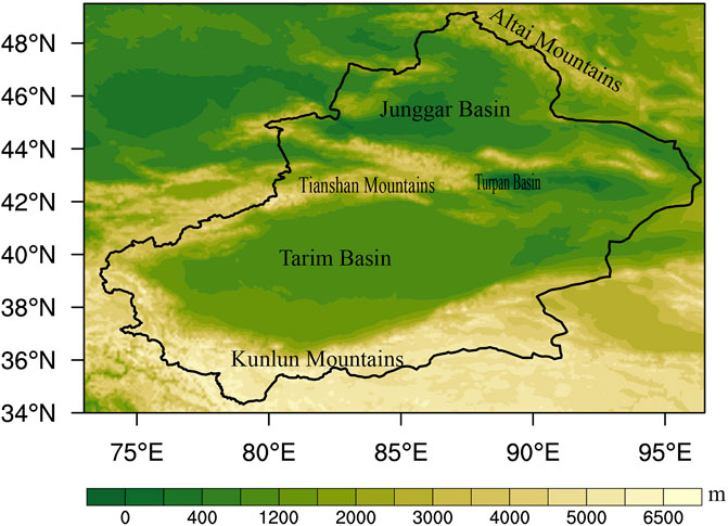
FIGURE 1. Study domain. The color bar represents the altitude of the terrain (m).
To calibrate the surface air temperature forecasts over Xinjiang, the training area for the U-net forecasts includes Xinjiang and the surrounding areas (73–96.5° E, 34–49.5° N). The corresponding topography is displayed in Figure 1. The GEFS reforecast datasets of surface air temperature with lead times of 1–7 days are provided by the NCEP/NOAA. The time range of the data, issued at 0:00 UTC, is from 1 January 2000 to 31 December 2019, and the horizontal resolution is 0.5 ° × 0.5 °. In addition, the ground truth used for verification is the ERA-5 dataset, which is often used as the observational data in studies of numerical model forecast calibrations (He et al., 2019; Hersbach et al., 2020). The detailed descriptions of forecast and observation datasets are given in Table 1.
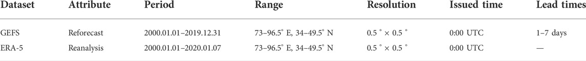
TABLE 1. Descriptions of forecast and observation datasets.
The observation and forecast data are divided into training period and forecast period. Correction equations are established according to the forecast and observations in the training period, and then the raw forecast in the forecast period is input into the correction equations to obtain the final calibration results. In ULR, the following equation is established on each grid point during the training period for the surface air temperature forecast with a specific forecast lead time:
where
where
The DAM is a correction method similar to a Kalman filter. It has the advantages of a small number of calculations and strong adaptability. It can effectively reduce the error through the lag average and is used operationally by the NCEP (Cui et al., 2012). The detailed calculation process is as follows:
On each grid point, the decreasing average error is obtained according to the predictions and observations during the training period:
where
Quantile mapping is a calibration method based on frequency distribution, which assumes that the predictions and observations are consistent in frequency distribution. Therefore, the transfer function between the predictions and observations can be established through quantiles to correct the model forecasts. Quantile mapping has been applied to the calibrations of several meteorological elements including precipitation and temperature (Maraun, 2013; Cannon et al., 2015). The detailed calculation process of quantile mapping in this paper is as follows:
On each grid point, first, the quantiles of the observations and predictions in the training period are calculated respectively. Then, a quantile-to-quantile segmented function is established to ensure that the predictions calibrated by the function have the same quantiles as the observations. Finally, the predictions in the prediction period is substituted into the segmented function to obtain the corrected forecast. The specific formula is as follows:
where
In this study, running training period is applied to the ULR, DAM and QM, obtaining the prediction of the day after the training period each time. The length of training period is tested over 10–60 days under different forecast lead times and the length of time corresponding to the minimum of average error is taken as the optimal length of training period to ensure the optimal correction results of the ULR, DAM and QM.
U-net, a CNN-based network, was first proposed in the image segmentation field. All the forecast and observational products used in this study are gridded data, which are similar to pixel-based images. Figure 2 shows the U-net network structure, which mainly consists of four types of components: convolution layers; pooling layers; upsampling layers; and skip connections. The whole network structure is shaped like the letter “U”. The left-hand is the downsampling side, that is, the encoding process, and the right-hand is the upsampling side, that is, the decoding process. The network has four depth layers. It should be noted that the depth of the U-net network can be adjusted manually. Different depths reflect different complexity of the model, and different correction results will be produced. In this paper, a series of parameters such as network depths, number of convolution kernels, the batch size and learning rate are continuously adjusted by minimizing the MSEs (the loss function) obtained from the training data in 2000–2017 and validation data in 2018. The structure of U-net shown in this paper is the final adjusted model.

FIGURE 2. Architecture of U-net. The left side of the U-shape is the downsampling side and the right side is the upsampling side.
During the downsampling process, raw GEFS forecast data with a size of 32 × 48×1 are input into the first layer as the raw predictor. After the first convolution process, the transformed versions of the raw predictor, called feature maps, are output with a size of 32 × 48×32. The convolution process does not change the area of the feature maps and the third dimension of the output represents the number of feature maps, which is consistent with the number of convolution kernels, that is, the number of channels, which increases with depth. The convolution kernels iterate through all the grid points in the inputs to extract data features. Weight-sharing within the convolution kernels can greatly reduce the number of parameters, increasing computational efficiency.
Each two convolution processes are followed by a pooling layer, which does not change the number of feature maps, but the area will be reduced to 1/n, where n is the size of the pooling kernels, equals to 2 in this study. This means that the area of the feature maps is halved after each pooling layer, leading to a decrease in the spatial resolution with depth. The convolution layers with different depths detect data features at different spatial resolutions, which is crucial in weather prediction because of the multiscale nature of weather phenomena and is the advantage of U-net over other machine learning methods. Convolution and pooling operations filter and reduce the dimensions of the inputs, retaining the main features of the raw data.
After three pooling processes, the raw data are compressed to the minimum before the upsampling process. Each green arrow represents one upsampling layer, where feature maps are upsampled to a higher spatial resolution via interpolation followed by convolution, after which the area of feature maps is doubled. Each upsampling layer is followed by a skip connection, represented by a gray arrow. Over the skip connection processes, high-resolution information from the downsampling side is preserved and carried to the upsampling side, which avoids the loss of fine-scale information. The features in the encoding process are reused in the decoding process through skip connections, which is another unique advantage of U-net that is not available in other machine learning methods. Feature maps from the upsampling layer contain higher-level abstractions and wider spatial context due to that they have passed through more hidden layers and have been upsampled from lower resolution. The upsampling process transforms high-resolution feature maps layer by layer and outputs the corrected model results.
The 2000–2017 data are input into U-net as the training dataset, and the 2018 and 2019 data are input as the validation and test datasets, respectively.
The details of the model are as follows. The rectified linear unit (ReLU) is used as the activation function in U-net:
The convolution kernel size is set to 3 × 3, which is commonly used. Adam is selected as the optimizer. The learning rate is set to
where
Four prediction test methods are adopted to make a quantitative evaluation of the temperature correction effect after statistical postprocessing, namely, the MAE, the mean absolute error skill score (MAESS), the hit rate (HR) and the pattern correlation coefficient (PCC). The corresponding calculation formulas are as follows:
where
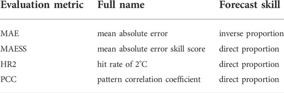
TABLE 2. The relationship between each evaluation metric and forecast skill.
All these error metrics aggregate the error evaluation results into composite scores, which lack interpretability. To solve this problem, based on the error decomposition method proposed by Hodson et al. (2021), the mean square error is decomposed into three interpretable error components in this study, namely, a bias term, a distribution term and a sequence term. Error diagnosis of each model is then carried out to indicate the direction required for further optimization. The specific algorithm is as follows.
For each grid point, the MSE is:
where
where
where
The difference between
In summary, the full error decomposition is:
where
Figure 3 shows the MAE, HR2 and PCC variations of the predicted surface air temperature averaged in Xinjiang by GEFS and the postprocessing procedures of ULR, the DAM, QM and U-net for lead times of 1–7 days. The multiple forecasts are generally characterized by consistent trends of increasing MAE values, while the HR2 and PCC values decrease. The four calibration methods all reduce the MAE and improve the HR2 and PCC relative to the raw GEFS forecasts for all lead times, but the skill improvement magnitudes of these four calibration methods are different.
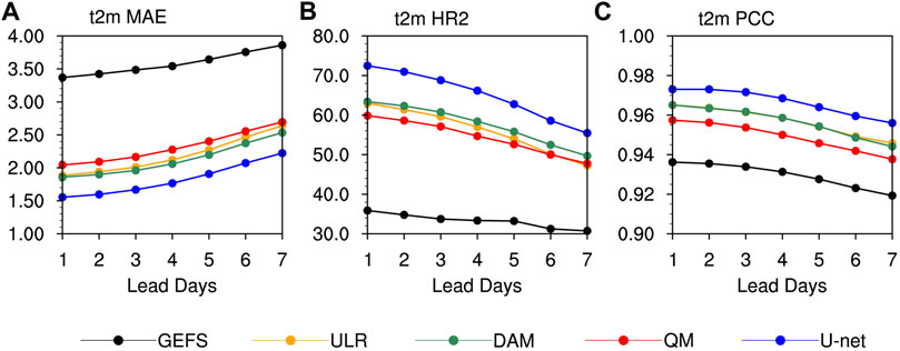
FIGURE 3. Variations in (A) MAE (°C), (B) HR2 (%); and (C) PCC of surface air temperature at lead times of 1–7 days derived from the GEFS, ULR, DAM, QM and U-net averaged in Xinjiang.
Among three conventional linear statistical postprocessing methods, QM has the least improvements while ULR and the DAM generally have similar calibration results for surface air temperature forecasts. The QM prediction results are significantly improved compared with the raw forecasts. Taking the forecast of the 1-day lead time as an example, the MAE, HR2 and PCC of GEFS are improved by QM from 3.37°C to 2.04°C, 35.88%–59.84% and 0.93 to 0.95, respectively. The ULR and DAM are superior to QM and advantages of DAM over ULR become more obvious with increasing lead times. U-net is characterized by the most manifest and consistent ameliorations among the four postprocessing methods. Taking the forecast of the 1-day lead time as an example, the MAE, HR2 and PCC of the DAM are 1.85°C, 63.40% and 0.96, respectively, whereas the same metrics of U-net are improved by 0.3°C, 9.08% and 0.01 respectively, indicating that it has some advantages over conventional linear methods in correcting the surface air temperature forecast.
Aiming at investigations on spatial characteristics of forecast performances, the MAE distributions derived from GEFS, ULR, DAM, QM and U-net are described in Figure 4 for surface air temperature forecasts, respectively, with lead times of 1, 4, and 7 days being taken as examples, as well as the corresponding MAESS distributions of the calibration methods in Figure 5. In terms of the raw GEFS forecasts, the largest MAEs mainly occur over the Altai Mountains, the Junggar Basin, the northern Tianshan Mountain, the Tarim Basin and the Kunlun Mountains, reaching up to 4.2°C even at the lead time of 1 day. This could be attributed to the insufficient descriptions of the altitude and complex terrain in the model, as well as a lack of observations in these regions.
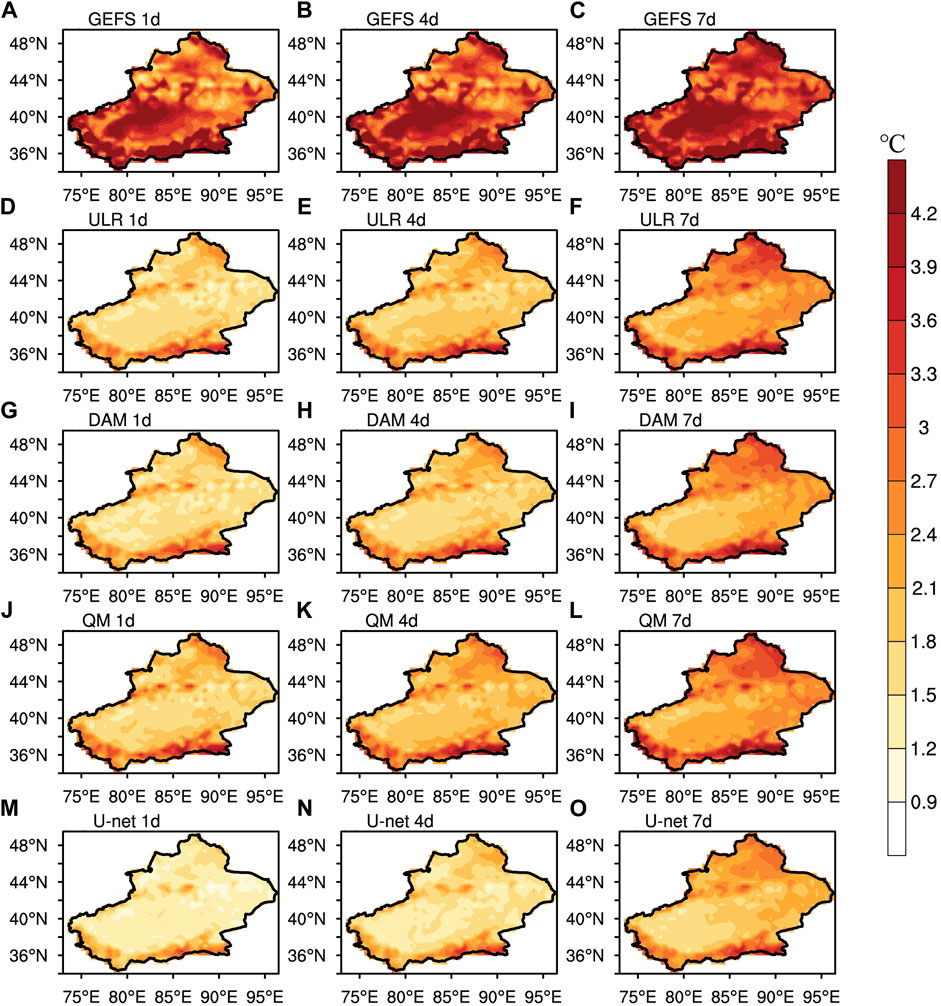
FIGURE 4. Spatial distributions of the MAE (°C) for surface air temperature forecasts with lead times of 1, 4, and 7 days derived from GEFS (A–C), ULR (D–F), DAM (G–I), QM (J–L) and U-net (M–O).
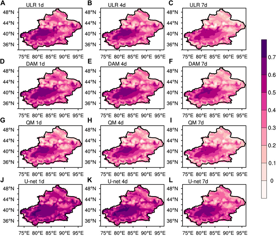
FIGURE 5. Spatial distributions of the MAESS of ULR (A–C), the DAM (D–F), QM (G–I) and U-net (J–L) to the raw GEFS forecast with lead times of 1, 4, and 7 days.
The four calibration methods are characterized by different magnitudes of ameliorations. The ULR improves the performance of raw GEFS forecasts over almost the whole of Xinjiang. About 30% of the area have an MAE <1.8°C at the lead time of 1 day. The most notable advances are located over the areas with the largest errors from raw forecasts. The spatial distributions of the MAESS show that the Tarim Basin has the maximum MAESS, that is, the main area of forecast improvement, where the MAESS reaches 0.4 at lead times of 1, 4 and 7 days. After calibration of the ULR, the largest MAEs mainly occur over the Altai Mountains, the Tianshan Mountains and the Kunlun Mountains, where the MAE is still ≥4.2°C in some districts. The skill improvement magnitudes of the ULR decreases with increasing lead times, expressed by an increasing MAE and decreasing MAESS. The regions with a negative MAESS increase significantly at the lead time of 7 days, mainly in northern Xinjiang, indicating that ULR no longer improves the forecasting skills of GEFS there. The calibration of the DAM is superior to ULR while QM is inferior to ULR, reflected by areas with MAE ≤1.8°C at the lead time of 1 day and regions with maximum MAESS at lead times of 1, 4, and 7 days compared with ULR. The MAESS after DAM reaches 0.6 in some areas of the Tarim Basin at the lead time of 7 days. The distribution of the maximum MAE corrected by three conventional methods are similar and the MAE maximum is still ≥4.2°C. There are fewer regions with a negative MAESS after calibration by the DAM than after ULR or QM.
The calibration with U-net is significantly improved compared with the DAM, which greatly reduces the MAE over almost the whole area of Xinjiang. About two-thirds of the area has an MAE ≤1.5°C at the lead time of 1 day, especially at the eastern and western boundaries of Xinjiang, where the MAE is reduced to ≤1.2°C. The MAESS is further improved compared with that after the DAM, with a maximum of ≥0.7 in the Tarim Basin at lead times of 1 and 4 days. In general, U-net shows most obvious ameliorations and all four calibration methods have better improvement in southern Xinjiang than in the north as a result of a larger MAESS in the south.
Figure 6 shows the spatial distributions of HR2 in forecasts of the GEFS, ULR, DAM QM and U-net for surface air temperature. As for the raw GEFS forecasts, the distributions show apparent differences between the southern and northern regions. The HR2 in most southern regions is ≤ 30% at each lead time, especially in the Tarim Basin and Kunlun Mountains, where GEFS shows limited forecast skills. By contrast, the HR2 reaches 40% in most regions of north Xinjiang and 60% in some districts at the lead time of 1 day, and 35% in more than half of north Xinjiang at the lead time of 7 days. The forecast skills of GEFS are generally poor and HR2 reaches 50% at each lead time in <20% of the regions.
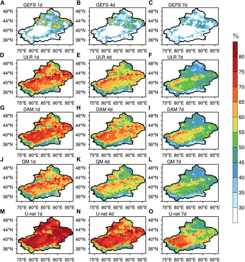
FIGURE 6. Spatial distributions of HR2s (%) for surface air temperature forecasts with lead times of 1, 4, and 7 days derived from GEFS (A–C), ULR (D–F), the DAM (G–I), QM (J–L) and U-net (M–O).
ULR and QM both significantly improves the HR2 throughout Xinjiang and have similar amelioration. About three-fourths of the area shows HR2 ≥55% at the lead time of 1 day and the maximum HR2 is distributed linearly from northeast to southwest, where it reaches 80% in some districts. In the Tarim Basin and Kunlun Mountains, where the raw GEFS forecast performance is poor, HR2 increases from ≤30 to 60 and 40%, respectively. With the increase in lead times, the magnitude of improvements of ULR and QM decreases, but the linear distribution of the HR2 maximum can still be identified, and HR2 in the Tarim Basin still reaches 50% at the lead time of 7 days.
For the DAM, the overall distribution of HR2 is similar to that of ULR and QM and the amelioration of DAM is slightly better. The area with HR2 ≥70% increases by 8% and 17% compared with that of ULR and QM respectively at the lead time of 1 day and the area with HR2 ≥55% increases by 13% and 12% compared with that of ULR and QM respectively at the lead time of 7 days.
The skill improvement magnitude of HR2 is much larger for U-net than the DAM. At the lead time of 1 day, HR2 reaches 70% in most areas of Xinjiang and 20% of the area has HR2 ≥80%, increasing by 18% compared with the DAM. At the lead time of 4 days, the area with HR2 ≥65% accounts for about 64%, increased by 40% compared with the DAM. At the lead time of 7 days, the HR2 in the Tarim Basin reaches 60% after calibration with U-net. The HR2 minimum is mainly located in the Junggar Basin and Kunlun Mountains, where the calibration methods show limited forecasting skills. Generally, the surface air temperature forecasting improvement of U-net in Xinjiang is much better than that of ULR, the DAM and QM.
In order to evaluate the cold and warm deviation of GEFS forecasts and optimal model calibrations, Figure 7 shows the error dispersion of the raw GEFS and U-net post-processed forecasts for the lead time of 1 day, including one histogram of the proportions of absolute errors in different ranges and two forecast-observation scatter diagrams. In forecast-observation scatter diagrams, the distance to the diagonal refers to the deviation of forecast to observation. The points above the diagonal represent warm biases, whereas the points below the diagonal represent cold biases. The histogram shows that GEFS absolute errors >5°C account for 24%, whereas GEFS absolute errors of ≤1°C account for less than <20%. From the scatter diagrams, the error dispersion of GEFS for surface air temperature is asymmetrical and there are more warm biases than cold biases, especially when the observations range between −40°C and −10°C.
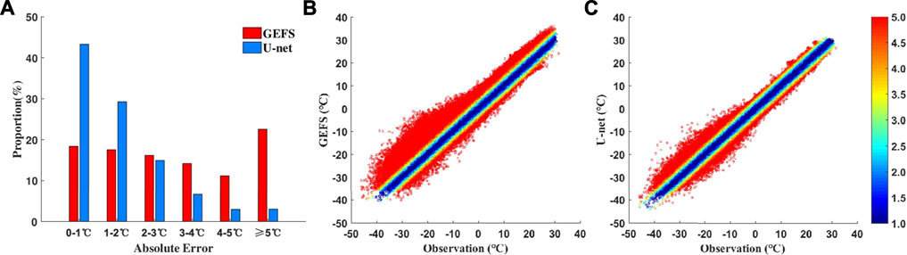
FIGURE 7. Error dispersion of the raw GEFS and U-net forecasts for surface air temperature at the 1-day lead time for the time period 1 January 2019-31 December 2019; the shading represents the scale of the errors.
The surface air temperature forecast skills are significantly improved after U-net calibration. The proportion of absolute errors ≤1°C greatly increases to 43%, an increase of 25% compared with GEFS, whereas the proportion of absolute errors >4°C greatly decreases to 6%, a decrease of 28% compared with GEFS. The warm biases are effectively eliminated after calibration and the error dispersion is more symmetrical.
All the evaluations discussed in Section 3.1 aggregate the calibrations into composite metrics, without understanding which aspects of the model performance are “good” or “bad”. In this section, based on the error decomposition method proposed by Hodson et al. (2021), the MSE is decomposed into three components, each representing a distinct concept. The bias term quantifies how well the model reproduces the mean of the observation. The sequence term represents the error caused by the forecasts leading or lagging the observations. The distribution term represents the error caused by differences in distribution between the forecasts and observations. Error decomposition helps researchers to diagnose the source of error from each forecasting scheme and to analyze the correcting effects of different schemes on the errors from different sources.
Figure 8 shows the MSE, the bias term (Bias2), the distribution term (Distribution) and the sequence term (Sequence) variations of the predicted surface air temperature averaged in Xinjiang by GEFS and the postprocessing procedures of ULR, DAM, QM and U-net for lead times of 1–7 days. The MSE of each scheme generally increases significantly with the lead time and the growth rate accelerates during lead times of 4–7 days. At the same lead time, GEFS always corresponds to the highest MSE. All four calibration methods significantly improve the forecast skills, among which QM has the highest MSE; ULR and the DAM almost have the same performance and U-net always corresponds to the lowest MSE.
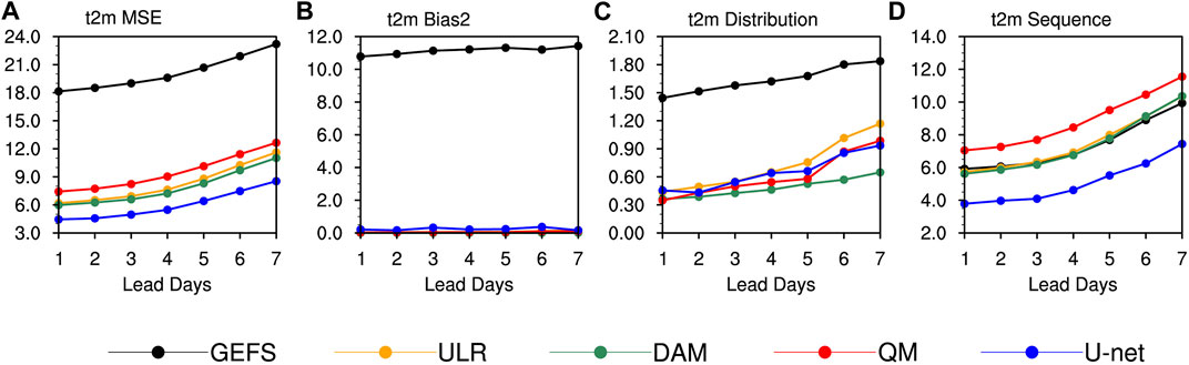
FIGURE 8. Variations in (A) MSE, (B) Bias2, (C) Distribution and (D) Sequence of surface air temperature at lead times of 1–7 days derived from GEFS, ULR, the DAM, QM and U-net averaged in Xinjiang (units:
After MSE decomposition, the variations in different terms show apparent differences. The Bias2 of GEFS is maintained at 11
Figure 9 shows the spatial distribution of the proportion of each error component in the MSE of GEFS, ULR, the DAM, QM and U-net to describe the main error sources in different regions under different forecasting schemes. There are clear differences in the sources of error between the north and south regions for the raw GEFS forecast. The bias term is the main source of error in the local surface air temperature forecast in most of the southern regions, accounting for >50% of MSE, whereas the sequence term is the main source of error in most of the northern regions, accounting for >50% of the MSE. The distribution term accounts for <30% of the MSE over almost the whole area of Xinjiang. The spatial distribution of the proportion of the sources of error changes significantly after all four postprocessing methods. Under each calibration scheme, the sequence error becomes the main source of error throughout Xinjiang, accounting for >50% of the MSE. There are slight differences in the distribution of proportions between different calibration methods. Throughout Xinjiang, the sequence terms of ULR, the DAM and QM account for >80% of the MSE and >90% in more than three-fourths of the regions. However, for U-net, although the sequence term still accounts for >80% in most regions, the area where the sequence term reaches 90% is smaller because the areas where Bias2 or Distribution account for 10% are larger than for ULR, the DAM and QM.
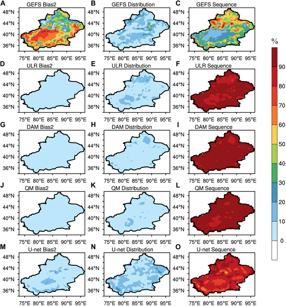
FIGURE 9. Spatial distribution of the proportion (%) of each decomposition component in the MSE at the lead time of 1 day derived from GEFS (A–C), ULR (D–F), the DAM (G–I), QM (J–L) and U-net (M–O).
Figure 10 shows the spatial distributions of Bias2 with lead times of 1, 4 and 7 days derived from GEFS, ULR, the DAM, QM and U-net to illustrate the improvements of each forecasting scheme on each MSE decomposition term. For the raw GEFS forecast, the Bias2 maximum, which reaches 12
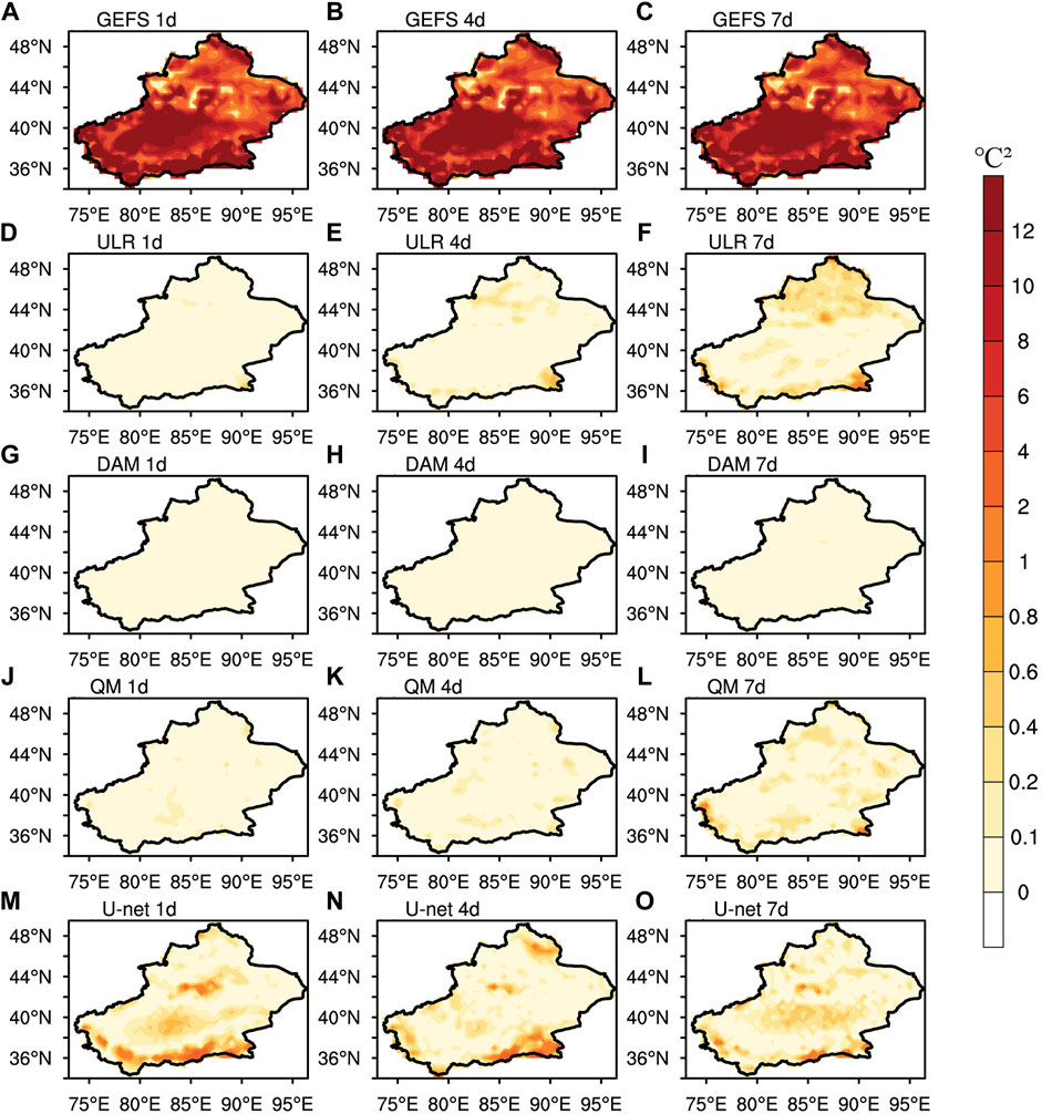
FIGURE 10. Spatial distributions of Bias2 (
Figure 11 shows the spatial distribution of the distribution term with lead times of 1, 4, and 7 days derived from GEFS, ULR, the DAM, QM and U-net. For the raw GEFS forecast, the spatial distribution of the distribution term barely changes with increasing lead times, with the maximum of >2.1
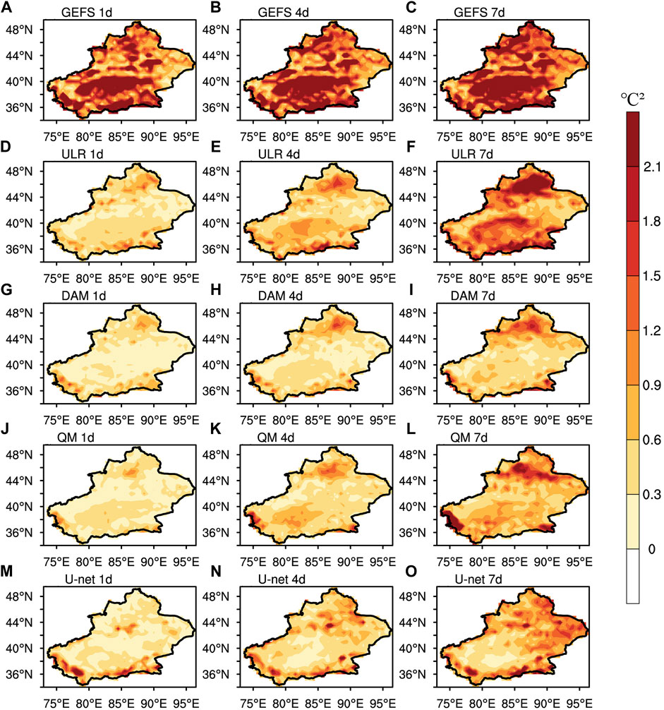
FIGURE 11. Spatial distributions of Distribution (
The skill improvement magnitude of Distribution in the DAM is superior to ULR. After the DAM, the areas with Distribution
The calibration performances of QM and U-net for Distribution are both between those of ULR and the DAM in general. In the Tarim Basin, the skill improvement magnitude of the distribution term after QM and U-net calibration is equivalent to that after the DAM and better than ULR. However, in the western Kunlun Mountains and Junggar Basin at the lead time of 7 days, the calibration of QM is inferior to DAM represented by the Distribution maximum of >2.1
Figure 12 shows the spatial distributions of the sequence term with lead times of 1, 4, and 7 days derived from GEFS, ULR, the DAM, QM and U-net. The maximum Sequence of the raw GEFS forecast is mainly located in the Altai Mountains, the Junggar Basin, and the Kunlun Mountains. With increasing lead times, the Sequence throughout Xinjiang increases and the area of maximum value expands. At the lead time of 7 days, the Sequence reaches 12
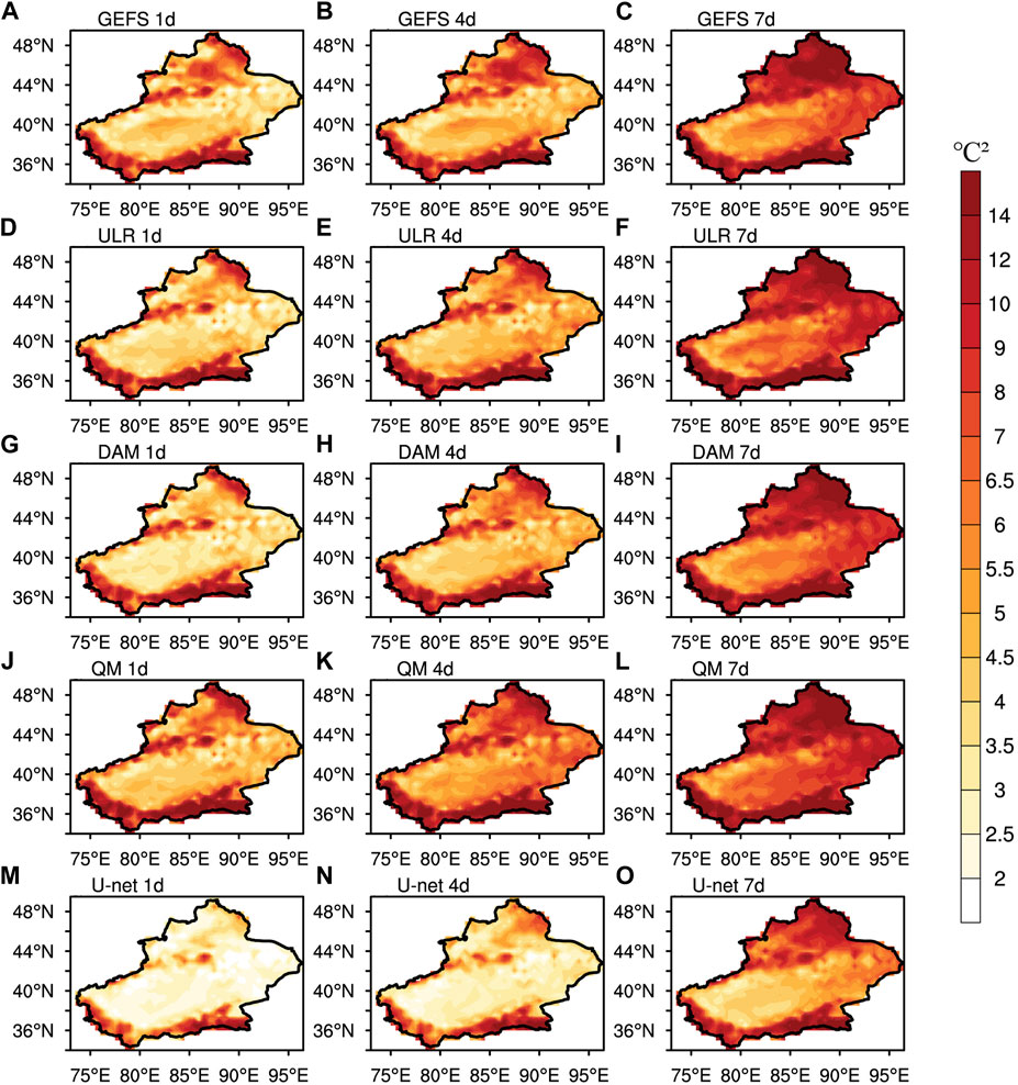
FIGURE 12. Spatial distributions of Sequence (
After ULR and the DAM, the Sequences in some areas of the Junggar and Tarim Basins are reduced at the lead time of 1 and 4 days, but the improvement in the Kunlun Mountains, where there are some negative improvements, is insufficient. At the lead time of 7 days, the areas of negative improvement after ULR and the DAM have significantly expanded in eastern Xinjiang and there are also many areas of negative improvement after ULR in the Tarim Basin. After QM, the areas of negative improvements are nearly throughout Xinjiang at all lead times, showing the least forecast skills. The performances of the three conventional calibration methods are generally not ideal in ameliorating the sequence term.
U-net can effectively reduce the sequence term over almost the whole area of Xinjiang, showing the most noticeable improvement. At the lead time of 1 day, the areas with Sequence
In this study, the forecast performance of the 2-m temperature from GEFS with lead times of 1–7 days in Xinjiang is evaluated. The deep learning neural network U-net is used to calibrate the raw GEFS forecasts. The applicability and capability of U-net to improve the surface air temperature forecasts are thoroughly examined and compared with the conventional postprocessing benchmarks of the ULR, the DAM and QM. Based on the MSE decomposition method, the sources of error and correcting effects of different schemes on the errors in different sources are analyzed. Associated results are obtained as follows.
The maximum MAE of the raw GEFS forecast is mainly located in the Altai Mountains, the Junggar Basin, the Tarim Basin, and the Kunlun Mountains and reaches
In general, all four calibration methods significantly improve the forecasting skills of the surface air temperature, with a lower MAE and higher HR2 and PCC. Among these methods, QM has the least improvements; ULR and DAM give quite similar results, whereas U-net shows the best improvement and can effectively eliminate the warm biases of the raw GEFS forecast. The magnitudes of improvement of the four calibrations are greater in southern Xinjiang than in the north.
For raw GEFS forecast, the bias term (Bias2) from the MSE decomposition is the main source of error and changes little with increasing lead times. The maximum Bias2 is mainly located in the Altai Mountains, the Tarim Basin and the Kunlun Mountains. This could be attributed to the insufficient descriptions of the altitude and complex terrain in the model, as well as a lack of observations in these regions. After the four postprocessing methods, the sequence term (Sequence) becomes the main source of error and shows an apparent increasing trend with increasing lead times. The maximum Sequence is mainly located in the Altai Mountains, the Junggar Basin and the Kunlun Mountains. All four postprocessing methods effectively reduces the bias and distribution terms of raw forecast, among which the DAM shows the best performance, but the differences among the four calibrations are small. Only U-net significantly reduces the sequence term; ULR and DAM barely give any improvement, whereas QM has obvious negative improvements, indicating an advantage of U-net over other three calibrations.
Dueben and Bauer (2018) showed that different neural networks may be applicable in different regions due to differences in geographical location and the terrain between each grid point. Zhi et al. (2021) indicated that the neural network considering the geographic information of each grid point performs better than the neural network without taking the geographic information into account for the probabilistic precipitation forecast. The errors of the surface air temperature forecast in the complex terrain of Xinjiang are mainly distributed in the mountains and basins. Geographical information (e.g., latitude, longitude and altitude) can also be fed into the neural network as training data in follow-up research to determine whether the forecasting skills can be further improved. In addition, the lead times in this study are 1–7 days, referred to as short and medium term; extended-range forecasts at longer timescales are always difficult in both theoretical research and practical operations (Zhu et al., 2021). It is therefore worth attempting to use U-net in an extended-range surface air temperature forecast for Xinjiang to determine whether it can still improve the forecasting skills. Other meteorological elements, especially discontinuous elements such as precipitation, can also be taken as forecast variables to test the applicability and capability of U-net in future studies.
The original contributions presented in the study are included in the article/supplementary material, further inquiries can be directed to the corresponding author.
YZ, XZ, YL and SZ contributed to conception and design of the study. YZ and YL performed the analyses. HT, AM, HZ and WH organized the database. YL and SZ was involved in the scientific interpretation and discussion. All authors contributed to manuscript revision, read, and approved the submitted version.
The study was jointly supported by the Collaboration Project of Urumqi Desert Meteorological Institute of China Meteorological Administration “Precipitation forecast based on machine learning”, the National Key R&D Program of China (Grant Nos. 2021YFC3000902 and 2017YFC1502002), the Basic Research Fund of CAMS (Grant No. 2022Y027) and the research project of Jiangsu Meteorological Bureau (Grant No. KQ202209).
The authors are grateful to ECMWF and NCEP/NOAA for their datasets.
The authors declare that the research was conducted in the absence of any commercial or financial relationships that could be construed as a potential conflict of interest.
All claims expressed in this article are solely those of the authors and do not necessarily represent those of their affiliated organizations, or those of the publisher, the editors and the reviewers. Any product that may be evaluated in this article, or claim that may be made by its manufacturer, is not guaranteed or endorsed by the publisher.
Bauer, P., Thorpe, A., and Brunet, G. (2015). The quiet revolution of numerical weather prediction. Nature 525, 47–55. doi:10.1038/nature14956
Boukabara, S. A., Krasnopolsky, V., and Stewart, J. Q. (2019). Leveraging modern artificial intelligence for remote sensing and NWP: Benefits and challenges. Bull. Am. Meteorol. Soc. 100, ES473–ES491. doi:10.1175/BAMS-D-18-0324.1
Cannon, A. J., Sobie, S. R., and Murdock, T. Q. (2015). Bias correction of GCM precipitation by quantile mapping: How well do methods preserve changes in quantiles and extremes? J. Clim. 28, 6938–6959. doi:10.1175/jcli-d-14-00754.1
Cui, B., Toth, Z., Zhu, Y., and Hou, D. (2012). Bias correction for global ensemble forecast. Weather Forecast. 27, 396–410. doi:10.1175/waf-d-11-00011.1
Dueben, P. D., and Bauer, P. (2018). Challenges and design choices for global weather and climate models based on machine learning. Geosci. Model Dev. 11, 3999–4009. doi:10.5194/gmd-11-3999-2018
Dupuy, F., Mestre, O., Serrurier, M., Burda, V. K., Zamo, M., Cabrera-Gutierrez, N. C., et al. (2021). ARPEGE cloud cover forecast postprocessing with convolutional neural network. Weather Forecast. 36, 567–586. doi:10.1175/waf-d-20-0093.1
Foresti, L., Sideris, I. V., Nerini, D., Beusch, L., and Germann, U. (2019). Using a 10-year radar archive for nowcasting precipitation growth and decay: A probabilistic machine learning approach. Weather Forecast. 34, 1547–1569. doi:10.1175/waf-d-18-0206.1
Geman, S., Bienenstock, E., and Doursat, R. (1992). Neural networks and the bias/variance dilemma. Neural Comput. 4, 1–58. doi:10.1162/neco.1992.4.1.1
Glahn, H. R., and Lowry, D. A. (1972). The use of model output statistics (MOS) in objective weather forecasting. J. Appl. Meteor. 11, 1203–1211. doi:10.1175/1520-0450(1972)011<1203:tuomos>2.0.co;2
Gupta, H. V., Kling, H., Yilmaz, K. K., and Martinez, G. F. (2009). Decomposition of the mean squared error and NSE performance criteria: Implications for improving hydrological modelling. J. Hydrology 377, 80–91. doi:10.1016/j.jhydrol.2009.08.003
Han, L., Chen, M., Chen, K., Chen, H., Zhang, Y., Lu, B., et al. (2021). A deep learning method for bias correction of ECMWF 24–240 h forecasts. Adv. Atmos. Sci. 38, 1444–1459. doi:10.1007/s00376-021-0215-y
Han, L., Sun, J., and Zhang, W. (2020). Convolutional neural network for convective storm nowcasting using 3-D Doppler weather radar data. IEEE Trans. Geosci. Remote Sens. 58, 1487–1495. doi:10.1109/tgrs.2019.2948070
He, D., Zhou, Z., Kang, Z., and Liu, L. (2019). Numerical studies on forecast error correction of GRAPES model with variational approach. Adv. Meteorology 2019, 1–13. doi:10.1155/2019/2856289
Hersbach, H., Bell, B., Berrisford, P., Hirahara, S., Horanyi, A., Munoz‐Sabater, J., et al. (2020). The ERA5 global reanalysis. Q. J. R. Meteorol. Soc. 146, 1999–2049. doi:10.1002/qj.3803
Hinton, G. E., and Salakhutdinov, R. R. (2006). Reducing the dimensionality of data with neural networks. Science 313, 504–507. doi:10.1126/science.1127647
Hodson, T. O., Over, T. M., and Foks, S. S. (2021). Mean squared error, Deconstructed. J. Adv. Model. Earth Syst. 13, e2021MS002681. doi:10.1029/2021ms002681
Hopson, T. M., and Webster, P. J. (2010). A 1–10-day ensemble forecasting scheme for the major river basins of Bangladesh: Forecasting severe floods of 2003–07. J. Hydrometeorol. 11, 618–641. doi:10.1175/2009jhm1006.1
Ji, L., Zhi, X., Simmer, C., Zhu, S., and Ji, Y. (2020). Multimodel ensemble forecasts of precipitation based on an object-based diagnostic evaluation. Mon. Weather Rev. 148, 2591–2606. doi:10.1175/mwr-d-19-0266.1
Jia, L., Zhang, Y., and He, Y. (2018). Research on error correction and intergration methods of maximum and minimum temperature forecast based on multi-model in Xinjiang. J. Arid Meteorology 36, 310–318. doi:10.11755/j.issn.1006-7639(2018)-02-0310
Krishnamurthy, V. (2019). Predictability of weather and climate. Earth Space Sci. 6, 1043–1056. doi:10.1029/2019ea000586
Krishnamurti, T. N., Kishtawal, C. M., LaRow, T. E., Bachiochi, D. R., Zhang, Z., Williford, C. E., et al. (1999). Improved weather and seasonal climate forecasts from multimodel superensemble. Science 285, 1548–1550. doi:10.1126/science.285.5433.1548
Krizhevsky, A., Sutskever, I., and Hinton, G. E. (2017). Imagenet classification with deep convolutional neural networks. Commun. ACM 60, 84–90. doi:10.1145/3065386
Lagerquist, R., McGovern, A., and Gagne, D. J. (2019). Deep learning for spatially explicit prediction of synoptic-scale fronts. Weather Forecast. 34, 1137–1160. doi:10.1175/waf-d-18-0183.1
Lagerquist, R., Stewart, J. Q., Ebert-Uphoff, I., and Kumler, C. (2021). Using deep learning to nowcast the spatial coverage of convection from himawari-8 satellite data. Mon. Weather Rev. 149, 3897–3921. doi:10.1175/MWR-D-21-0096.1
LeCun, Y., Bengio, Y., and Hinton, G. (2015). Deep learning. Nature 521, 436–444. doi:10.1038/nature14539
Li, B., and Zhi, X. (2012). Comparative study of four correction schemes of the ECMWF surface temperature forecasts. Meteorol. Mon. 38, 897–902. doi:10.7519/j.issn.1000-0526.2012.8.001
Li, H., Yu, C., Xia, J., Wang, Y., Zhu, J., and Zhang, P. (2019). A model output machine learning method for grid temperature forecasts in the beijing area. Adv. Atmos. Sci. 36, 1156–1170. doi:10.1007/s00376-019-9023-z
Livingston, R. L., and Schaefer, J. T. (1990). On medium-range model guidance and the 3-5 Day extended forecast. Weather Forecast. 5, 361–376. doi:10.1175/1520-0434(1990)005<0361:omrmga>2.0.co;2
Lorenz, E. N. (1982). Atmospheric predictability experiments with a large numerical model. Tellus 34, 505–513. doi:10.1111/j.2153-3490.1982.tb01839.x
Lorenz, E. N. (1963). Deterministic nonperiodic flow. J. Atmos. Sci. 20, 130–141. doi:10.1175/1520-0469(1963)020<0130:dnf>2.0.co;2
Lorenz, E. N. (1969). The predictability of a flow which possesses many scales of motion. Tellus 21, 289–307. doi:10.1111/j.2153-3490.1969.tb00444.x
Lyu, Y., Zhi, X., Zhu, S., Fan, Y., and Pan, M. (2021). Statistical calibrations of surface air temperature forecasts over East Asia using pattern projection methods. Weather Forecast. 36, 1661–1674. doi:10.1175/waf-d-21-0043.1
Maraun, D. (2013). Bias correction, quantile mapping, and downscaling: Revisiting the inflation issue. J. Clim. 26, 2137–2143. doi:10.1175/jcli-d-12-00821.1
Mecikalski, J. R., Williams, J. K., Jewett, C. P., Ahijevych, D., LeRoy, A., and Walker, J. R. (2015). Probabilistic 0-1-h convective initiation nowcasts that combine geostationary satellite observations and numerical weather prediction model data. J. Appl. Meteorology Climatol. 54, 1039–1059. doi:10.1175/jamc-d-14-0129.1
Murphy, A. H. (1988). Skill scores based on the mean square error and their relationships to the correlation coefficient. Mon. Weather Rev. 116, 2417–2424. doi:10.1175/1520-0493(1988)116<2417:ssbotm>2.0.co;2
Pan, M., Zhi, X., Liu, Z., Zhu, S., Lyu, Y., and Zhu, D. (2022). Statistical calibrations to improve the 2-5-year prediction skill for SST over the North Atlantic. Meteorol. Atmos. Phys. 134, 52–14. doi:10.1007/s00703-022-00888-4
Peng, T., Zhi, X., Ji, Y., Ji, L., and Tian, Y. (2020). Prediction skill of extended range 2-m maximum air temperature probabilistic forecasts using machine learning post-processing methods. Atmosphere 11, 823–835. doi:10.3390/atmos11080823
Peng, X., Che, Y., and Chang, J. (2013). A novel approach to improve numerical weather prediction skills by using anomaly integration and historical data. J. Geophys. Res. Atmos. 118, 8814–8826. doi:10.1002/jgrd.50682
Rasp, S., and Lerch, S. (2018). Neural networks for post-processing ensemble weather forecasts. Mon. Weather Rev. 146, 3885–3900. doi:10.1175/mwr-d-18-0187.1
Reichstein, M., Camps-Valls, G., Stevens, B., Jung, M., Denzler, J., Carvalhais, N., et al. (2019). Deep learning and process understanding for data -driven Earth system science. Nature 566, 195–204. doi:10.1038/s41586-019-0912-1
Ronneberger, O., Fischer, P., and Brox, T. (2015). “U-net: Convolutional networks for biomedical image segmentation,” in Proc. 18th int. Conf. On medical image computing and computer-assisted intervention (Munich, Germany: Springer).
Screen, J. A., Deser, C., and Sun, L. (2015). Reduced risk of North American cold extremes due to continued Arctic sea ice loss. Bull. Am. Meteorological Soc. 96, 1489–1503. doi:10.1175/bams-d-14-00185.1
Sha, Y., Gagne, D. J., West, G., and Stull, R. (2020a). Deep-learning-based gridded downscaling of surface meteorological variables in complex terrain. Part I: Daily maximum and minimum 2-m temperature. J. Appl. Meteorology Climatol. 59, 2057–2073. doi:10.1175/jamc-d-20-0057.1
Sha, Y., Gagne, D. J., West, G., and Stull, R. (2020b). Deep-learning-based gridded downscaling of surface meteorological variables in complex terrain. Part II: Daily precipitation. J. Appl. Meteorology Climatol. 59, 2075–2092. doi:10.1175/jamc-d-20-0058.1
Slingo, J., and Palmer, T. (2011). Uncertainty in weather and climate prediction. Phil. Trans. R. Soc. A 369, 4751–4767. doi:10.1098/rsta.2011.0161
Sulikowska, A., and Wypych, A. (2020). How unusual were June 2019 temperatures in the context of European climatology? Atmosphere 11, 697. doi:10.3390/atmos11070697
Tao, Y., Gao, X., Hsu, K., Sorooshian, S., and Ihler, A. (2016). A deep neural network modeling framework to reduce bias in satellite precipitation products. J. Hydrometeorol. 17, 931–945. doi:10.1175/jhm-d-15-0075.1
Vannitsem, S., Bremnes, J. B., Demaeyer, J., Evans, G. R., Flowerdew, J., Hemri, S., et al. (2020). Statistical postprocessing for weather forecasts - review, challenges and avenues in a big data world. Bull. Am. Meteorological Soc. 102, E681–E699. doi:10.1175/bams-d-19-0308.1
Vashani, S., Azadi, M., and Hajjam, S. (2010). Comparative evaluation of different post processing methods for numerical prediction of temperature forecasts over Iran. Res. J. Environ. Sci. 4, 305–316. doi:10.3923/rjes.2010.305.316
Xue, H., Shen, X., and Chou, J. (2015). An online model correction method based on an inverse problem: Part I—model error estimation by iteration, Model error estimation by iteration. Adv. Atmos. Sci. 32, 1329–1340. doi:10.1007/s00376-015-4261-1
Yuan, H., Mcginley, J. A., Schultz, P. J., Anderson, C. J., and Lu, C. (2006). Short-range precipitation forecasts from time-lagged multimodel ensembles during the HMT-West-2006 campaign. J. Hydrometeorol. 9, 477–491. doi:10.1175/2007jhm879.1
Zhang, L., Sielmann, F., Fraedrich, K., Zhu, X., and Zhi, X. (2015). Variability of winter extreme precipitation in southeast China: Contributions of SST anomalies. Clim. Dyn. 45, 2557–2570. doi:10.1007/s00382-015-2492-6
Zhi, X., Qi, H., Bai, Y., and Lin, C. (2012). A comparison of three kinds of multimodel ensemble forecast techniques based on the TIGGE data. Acta Meteorol. Sin. 26, 41–51. doi:10.1007/s13351-012-0104-5
Zhi, X., Zhang, K., and Tian, Y. (2021). Probabilistic precipitation forecast in East and South China based on neural network and geographic information. Trans. Atmos. Sci. 44, 381–393. doi:10.13878/j.cnki.dqkxxb.20210117001
Zhu, S., Ge, F., Fan, Y., Zhang, L., Sielmann, F., Fraedrich, K., et al. (2020). Conspicuous temperature extremes over southeast asia: Seasonal variations under 1.5 °C and 2 °C global warming. Clim. Change 160, 343–360. doi:10.1007/s10584-019-02640-1
Keywords: temperature forecast, calibration, xinjiang, deep learning, U-net, error decomposition
Citation: Zhu Y, Zhi X, Lyu Y, Zhu S, Tong H, Mamtimin A, Zhang H and Huo W (2022) Forecast calibrations of surface air temperature over Xinjiang based on U-net neural network. Front. Environ. Sci. 10:1011321. doi: 10.3389/fenvs.2022.1011321
Received: 04 August 2022; Accepted: 07 September 2022;
Published: 20 September 2022.
Edited by:
Ying Chen, Paul Scherrer Institut, SwitzerlandReviewed by:
Ju Liang, University of Exeter, United KingdomCopyright © 2022 Zhu, Zhi, Lyu, Zhu, Tong, Mamtimin, Zhang and Huo. This is an open-access article distributed under the terms of the Creative Commons Attribution License (CC BY). The use, distribution or reproduction in other forums is permitted, provided the original author(s) and the copyright owner(s) are credited and that the original publication in this journal is cited, in accordance with accepted academic practice. No use, distribution or reproduction is permitted which does not comply with these terms.
*Correspondence: Xiefei Zhi, emhpQG51aXN0LmVkdS5jbg==
Disclaimer: All claims expressed in this article are solely those of the authors and do not necessarily represent those of their affiliated organizations, or those of the publisher, the editors and the reviewers. Any product that may be evaluated in this article or claim that may be made by its manufacturer is not guaranteed or endorsed by the publisher.
Research integrity at Frontiers
Learn more about the work of our research integrity team to safeguard the quality of each article we publish.