
94% of researchers rate our articles as excellent or good
Learn more about the work of our research integrity team to safeguard the quality of each article we publish.
Find out more
ORIGINAL RESEARCH article
Front. Environ. Sci., 29 September 2022
Sec. Atmosphere and Climate
Volume 10 - 2022 | https://doi.org/10.3389/fenvs.2022.1005575
This article is part of the Research TopicAtmospheric Disturbances: Responses to Phenomena from Lithosphere to Outer SpaceView all 5 articles
 Aleksandra Nina1*
 Pier Francesco Biagi2
 Sergey Pulinets3
 Giovanni Nico4Srđan T. Mitrović5Vladimir M. Čadež6
 Milan Radovanović7,8Marko Urošev7Luka Č. Popović6,9,10
Recent research shows reductions in the VLF signal noise amplitude that begin before particular earthquakes whose epicentres are more than 100 km away from the signal propagation path. In this paper, we extend this research to studying the noise amplitude during periods of intense seismic activity in a localized area. We analyse variations in the VLF signal noise amplitude over a period of 10 days (25 October–3 November 2016) when 981 earthquakes with the minimum magnitude of 2 occurred in Central Italy. Out of these events, 31 had the magnitude equal or greater than 4, while the strongest one had the magnitude of 6.5. We observe the VLF signal emitted by the ICV transmitter located in Sardinia (Italy) and recorded in Belgrade (Serbia). Bearing in mind that the trajectory of this signal crosses the area in which the observed earthquakes occurred, we extend the existing research to study of variations in the noise amplitude of the signal propagating at short distances from the epicentres of the considered earthquakes. In addition, we analyse the impact of a large number earthquakes on characteristics of the noise amplitude and its reductions before particular events. In order to examine the localization of the recorded changes, we additionally analysed the noise amplitude of two reference signals emitted in Germany and Norway. The obtained results show the existence of the noise amplitude reduction preceding individual strong or relatively strong earthquakes, and earthquakes followed by others that occurred in a shorter time interval. However, the additional noise amplitude reductions are either not pronounced or they do not exist before the considered events in periods of the reduced noise amplitude remain from previous earthquakes. Reductions in noise amplitudes for all observed signals indicate a larger perturbed area through which they spread or its closer location to the receiver. The analysis of daily values of parameters describing the noise amplitude reveals their variations start up to 2 weeks before the seismically active period occurs.
In a large number of scientific studies published in this and the previous century, different types of ionospheric disturbances that precede earthquakes (EQs) are shown (Davies and Baker, 1965; Leonard et al., 1965; Yuen et al., 1969; Calais and Minster, 1998; Maekawa et al., 2006; Sasmal and Chakrabarti, 2009; Chakrabarti et al., 2010; Oyama et al., 2016; Xiong et al., 2021; He et al., 2022; Molina et al., 2022). The repetition of the same or very similar characteristics of these disturbances indicates the possibility that they are precursors of earthquakes, which is why a relevant both theoretical and experimental research is of great importance. In the first case, studies provide several theoretical explanations for the relationship between ionospheric disturbances and lithospheric processes associated with earthquakes, and they are based on thermal and chemical mechanisms as well as on generation of acoustic and electromagnetic waves, and quasi constant local electric field (Sorokin and Yashchenko, 1999; Pulinets and Boyarchuk, 2004; Liperovsky et al., 2008; Korepanov et al., 2009; Pulinets and Ouzounov, 2011; Fu et al., 2015). On the other hand, the observations are based on remote sensing of the high (using ionosonde/digisonde and radar) and lower (using very low/low frequency (VLF/LF) radio signals) ionosphere as well as integral information about the entire ionosphere obtained by the Global Navigation Satellite System (GNSS) signals (Biagi et al., 2001b, 2011; Hegai et al., 2006; Perrone et al., 2018). In addition, measurements by satellites orbiting in the ionosphere (e.g., Detection of Electro-Magnetic Emissions Transmitted from Earthquake Regions (DEMETER) satellite) are used for relevant studies (Němec et al., 2009).
Previous studies indicate that typical perturbations (variations of the electron density (positive and negative) at specific altitudes of the ionosphere registered by ionosondes, the total electron content (TEC) variations registered by GNSS receivers, changes in the VLF/LF signal amplitude (or phase), its periodic fluctuations and the “terminator time” shift) are registered in all ionospheric regions mostly a few days before the occurrence of stronger earthquakes (Hayakawa, 1996; Molchanov et al., 1998; Biagi et al., 2001b, 2006; Miyaki et al., 2001; Molchanov et al., 2001; Pulinets and Boyarchuk, 2004; Rozhnoi et al., 2004; Yamauchi et al., 2007; Hayakawa et al., 2010; Liu et al., 2018; Perrone et al., 2018; Pulinets et al., 2022). However, recent research presented in Nina et al. (2020) and Nina et al. (2021a) points out a possibility for a new type of precursor that occurs up to a few tens of minutes before an EQ (including some cases of weak earthquakes whose magnitude can be less than 3) and manifests itself through a reduction in the VLF signal amplitude and phase noise, respectively. These studies present analyses of several EQs whose epicentres were relatively close to the considered signal propagation path. In these analysed cases, the detected individual reductions can be clearly associated with individual EQs. In other words, the disturbance in the environment in which the signal propagates either ends quickly enough and do not affect disturbances that could potentially be associated with further EQs or is further amplified before an another event. A possible explanation for this may be the fact that the analysed earthquakes occurred in several remote locations (Serbia, Italy, Tyrrhenian Sea and Western Mediterranean Sea). However, the question arises as to how a large number of EQ events whose epicentres are located in close locations and that occur in a relatively short time period affect the signal noise properties. The importance of this issue can be seen in the fact that in the DHO and GQD signals with a small noise amplitude during the time periods observed in the study Nina et al. (2020) no reduction of the noise amplitude was recorded, which, consequently, requires the examination of the existence of an additional reduction of this parameter if it is already significantly reduced by some previous EQ. The analysis of this issue is the main aim of this paper. In addition, the aims of this research are to explore the VLF signal prior the considered EQs in order to confirm our finding of the noise amplitude reduction in the case of EQs that occurred during the period when the noise amplitude corresponds to that in quiet conditions and, for the first time, to explore the daily characteristics of the VLF signal noise amplitude in time periods before, during and after the considered intensive seismic activity.
In this study, we analyse the time evolution of the noise amplitude of the ICV signal transmitted in Italy and recorded in Serbia in the period from 25 October to 3 November 2016 which was the time period of intense seismic activity (PISA). During this period there were 981 earthquakes in Central Italy of minimum magnitude 2, out of which there were 31 cases with magnitudes equal or greater than 4. In addition, we analyse daily characteristics of the noise amplitude in the time period from 1 October to 22 December in order to examine long-term variations around intense seismic activity located at a small area. To study localization of the perturbed atmospheric part, we analyse two additional VLF signals emitted by the DHO (Germany) and JXN (Norway) transmitters and received in Belgrade, Serbia.
The paper is organised as follows. The descriptions of observations, considered events, and the applied procedures for data processing are presented in Section 2. Section 3 shows the obtained results and their discussion. Finally, the conclusions of this study and the list of the opened questions are given in Section 4.
The study presented in this paper is based on the processing of the VLF signal amplitudes recorded by the Absolute Phase and Amplitude Logger (AbsPAL) receiver in Belgrade, Serbia (44.8 N, 20.4 E). The data recorded by this receiver are used in many analyses (Žigman et al., 2007; Grubor et al., 2008; Kolarski et al., 2011). Here, we analyse three signals emitted by the ICV, DHO and JXN transmitters located in Isola di Tavolara, Sardinia, Italy (40.92 N, 9.73 E), Rhauderfehn, Germany (53.10 N, 7.60 E) and Kolsas, Norway (59.91 N, 10.52 E), respectively. Their propagation paths are shown in Figure 1A.
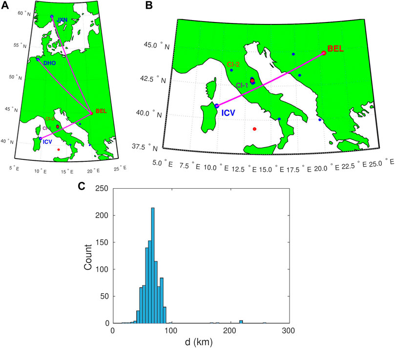
FIGURE 1. (A): Propagation paths of the VLF signals recorded by the Belgrade receiver station (BEL) in Serbia and emitted by the ICV, DHO and JXN transmitters located in Italy, Germany and Norway, respectively (solid pink lines). (B): Zoomed view of the left map for the ICV signal. Blue, red and black dots mark the epicentres of earthquakes of magnitude 4 ≤ M < 5 (blue dots), 5 ≤ M < 6 (red dots) and M ≥ 6 (black dots) that occurred in the period from 25 October to 3 November 2016. The areas in Central Italy where the epicentres of the earthquakes recorded in the observed period are located are marked with CI-1 and CI-2. (C): Distribution of the distance of the earthquake epicentre from the ICV signal propagation path.
The focus of this research is on the ICV signal amplitude processing because, as the map shows, its propagation path to Belgrade is closest to the epicentres of the observed set of earthquakes marked as blue, red and black points depending of their magnitudes (a zoomed map view of the signal propagation area is given in the upper right panel). In addition, a study given in Nina et al. (2020) indicates the appropriate noise amplitude reductions for this signal, and, consequently, shows that it is suitable for relevant analyses. This is important because the influence of the signal characteristics on the possibility of detecting the considered specified form of amplitude change has not been investigated yet, and by choosing this signal we eliminate the possibility of no detection of the observed change due to e.g. insufficient sensitivity of the selected signal to atmospheric noise variations.
We analyse the signals emitted by the DHO and JXN transmitters in order to examine the influence of the receiver, and electronic and electrical devices close to it on the signal noise amplitude, and the localization of the detected changes. Here, we point out that variations in the signal emission relevant for the study are eliminated by analysing its amplitude recorded by the receiver located in Kilpisjärvi, Norway (see Section 2.3).
In the detailed analysis of the ICV signal amplitude, we observe the time period from 25 October to 3 November 2016 when seismic activity in Central Italy was very intense. In Figure 1, we show a map of the area where the observed signal propagates, and the epicentres of EQs that occurred during the analysed time period, out of which 981 (with the magnitude, M, equal or greater than 2) occurred in Central Italy. For clarity, we show the epicentres of earthquakes of minimum magnitudes 3.9 (blue dots), 5 (red circle) and 6 (black circles) on this map. As can be seen in the map, these epicentres are grouped into two localized areas marked as CI-1 and CI-2 (the maximum earthquake magnitude in this area is 3.9, so we included this value in the epicentre display in the map). The histogram of the distances d between the epicentres of all considered EQs and the signal propagation path is shown in Figure 1C where one can see that d is smaller than 100 km in almost all (more than 99%) cases. The number of the EQ events with 40 km
Considering that the epicentres of EQs that occurred in the CI-2 area are significantly further from the signal propagation path (d is between 168 and 259 km) than those occurred in the CI-1 area (d is below 100 km), and that their magnitudes are below 4, we focus on evens in the CI-1 area. A zoomed view of the map for this area with 31 EQ epicentre locations (for M ≥ 4) and part of the observed signal path are given in the left panel, while the numbers of EQ events per day with magnitudes between 2 and 3, 3 and 4, 4 and 5, 5 and 6, and greater than 6 are shown in Figure 2B. The list of analysed 31 earthquakes (magnitudes of 4) with their characteristics (times of their events, epicentre locations, depths, magnitude values and types, and epicentre distances from the ICV signal propagation path) is given in Table 1.
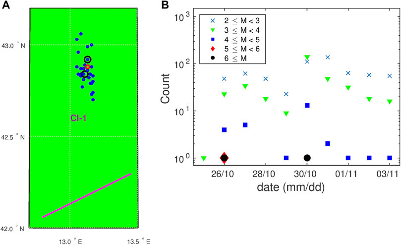
FIGURE 2. (A): A zoomed view of the map shown in Figure 1 that includes the earthquake epicentres in the CI-1 area and a part of the ICV signal propagation path between the transmitter in Sardinia, Italy, and the receiver in Belgrade, Serbia. (B): Time evolution of the number of earthquakes of magnitudes 2 ≤ M < 3 (x), 3 ≤ M < 4 (green triangles), 4 ≤ M < 5 (blue squares), 5 ≤ M < 6 (red diamond) and 6 ≤ M (black circles) in the CI-1 area during the observed time period.
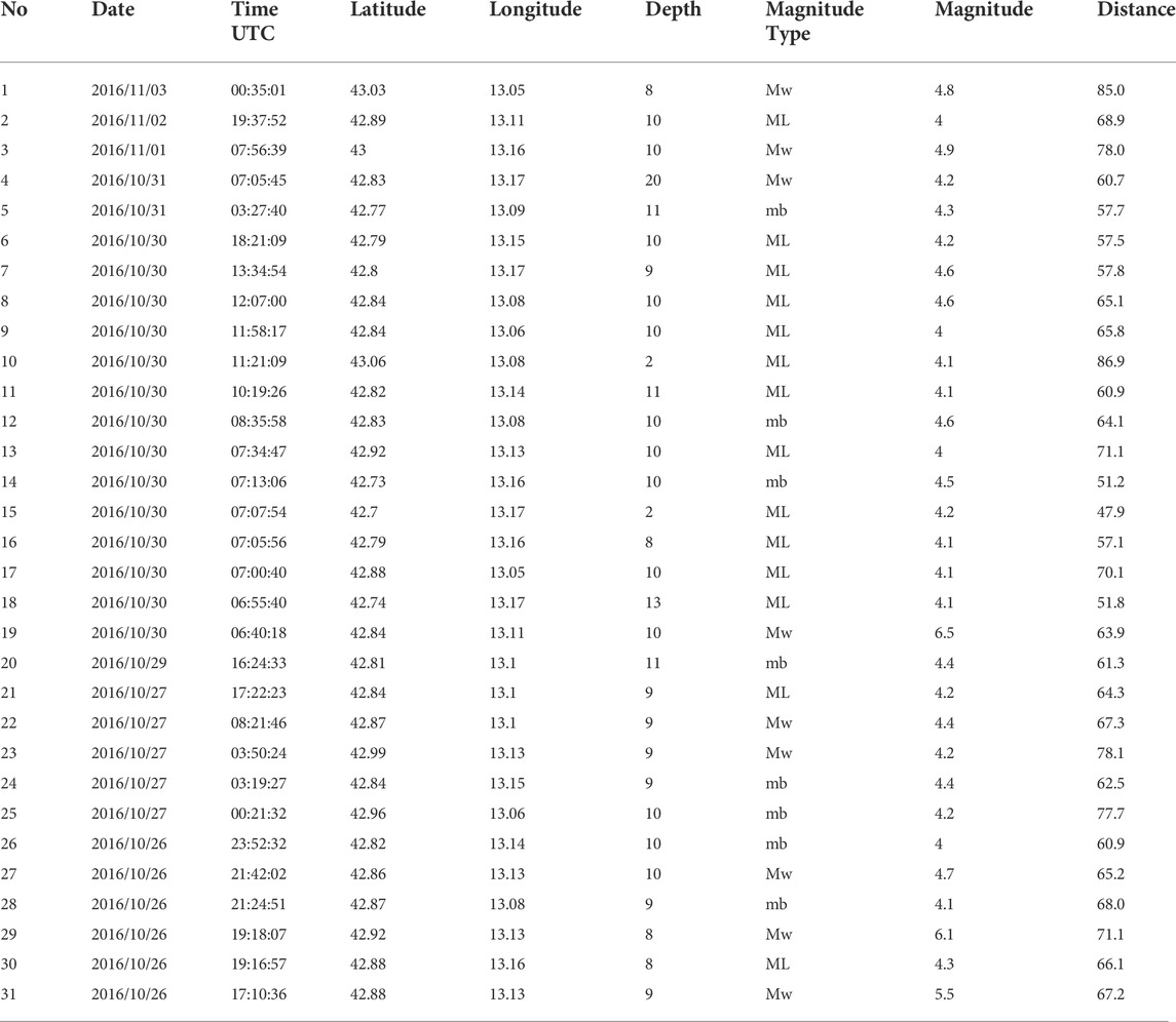
TABLE 1. List of the main studied earthquakes. Data for EQ date, time t, epicentre locations (latitude (LAT) and longitude (LON)) and magnitudes (M) are given in http://www.emsc-csem.org/Earthquake/. Distances between the EQ epicentres and signal propagation path are indicated as d.
As one can see in the map shown in Figure 1, the upper right panel, two additional EQs also occurred relatively close to the considered signal propagation path (in Bosnia and Herzegovina). Their magnitudes are 4.2 (31 October 2016, 09:38:13 UT, (43.26N,17.88E)) and 3.9 (3 November 2016, 15:04:03 UT, (44.82N,17.3E)). In the first case, no reduction of Anoise is recorded, while in the period around the second event the ICV signal is not recorded in Belgrade. In the observed period, there were additional two EQs of magnitudes of 2.6 and 2.5 in Bosnia and Herzegovina, and Serbia, respectively. In the first case, the analysed reduction is not recorded, while, in the second case, the time of EQ is in the period of occurrences of two EQs of higher magnitudes (4.6 and 3.9) in the CI-1 area which are much more likely to be associated with the corresponding detected Anoise reduction. The strongest EQ outside Central Italy of magnitude 5.8 occurred in the Tyrrhenian Sea (28 October, 20:02:49 UT, (39.35N,13.44E)). As will be seen in Section 3, Anoise is low throughout the day and although its slight reduction in the period around this EQ is visible, it is not possible to reliably link these two phenomena.
Based on the previous analysis, it can be concluded that the noise amplitude reductions can be related to the EQs that occurred in the CI-1 area and that other EQ events do not significantly affect the presented analysis.
In addition to the detailed analysis of the ICV signal amplitude for the indicated 10 days, we analysed the period from 1 October to 22 December to examine long-term variations around the seismological active period.
As stated in the literature (Biagi et al., 2011; Nina et al., 2020), there are numerous causes of variations in signal characteristics. They refer both to natural sources of disturbances and to technical changes in the emission and reception of signals due to, for example, electric or electronic devices operating nearby the receiver, electric cables without good shielding, amateur radios operating in the zone, an improperly grounded receiver, or natural electromagnetic emissions from nearby faults or micro-fractured zones. For this reason, it is necessary to check the presence of influence of these factors on the signal characteristics important for this study.
• Natural conditions. The main potential natural causes of changes in a VLF signal propagation are related to meteorological and geomagnetic conditions, and variations in radiation from the Sun and other sources in the Universe.
• Meteorological conditions can cause disturbances in signal characteristics of different durations. However, typical signal variations caused by lightning (see, for example, Wang et al. (2020) and references therein) do not have the same characteristics as those analysed in Nina et al. (2020) as a potential EQ precursor. In addition, there were no significant meteorological events in the area near the ICV signal route from Sardinia to Belgrade in the observed period according to the European Severe Weather Database (https://eswd.eu/cgi-bin/eswd.cgi). The only recorded north wind was on 2 November 2016.
• Geomagnetic conditions. The values of the Kp index were below 5 during this time, except in seven and three three-hour periods when they were
• Extraterrestrial electromagnetic radiation. Changes in the D-region electron density (the plasma parameter that is significant for a VLF signal propagation) are dominantly influenced by the solar hydrogen Lyα line in quiet conditions (Mitra, 1974; Nina et al., 2021b) and the soft X-radiation produced during solar X-ray flares (Thomson et al., 2005; Kolarski et al., 2011; Basak and Chakrabarti, 2013; Schmitter, 2013; Ammar and Ghalila, 2016; Chakraborty and Basak, 2020). In both cases, these impacts are significant during the daytime period. Based on the obtained noise amplitude values in Nina et al. (2020), it can be concluded that the noise amplitude of the observed signal is not affected by the daily variations of the mentioned Lyα radiation. In addition, during the observed period, no solar X-ray flares of class C and stronger, which can affect VLF signal characteristics, were recorded (https://hesperia.gsfc.nasa.gov/goes/goes_event_listings/). Based on this, we can conclude that solar radiation cannot be the cause of the significant variations in the noise amplitude analysed in this study.
The changes in the signal that are indicated as the detection of gamma ray burst in Inan et al. (2007) are not recorded, while those shown in Nina et al. (2015) do not correspond to the changes analysed in this study.
• Non-natural conditions. Amplitude variations that result in reductions of its noise amplitude can also be consequences of variations in the signal emission and/or reception. In order to eliminate the presence of these influences, we analyse the amplitude of the ICV signal recorded by the Kilpisjärvi ULTRA Data receiver (to check variations in the emission of the observed ICV signal) and the DHO and JXN signals emitted in Germany and Norway, respectively, and received by the AbsPAL receiver in Belgrade (to check variations in the reception of the signal by the used receiver). Comparisons with the analysed ICV signal noise amplitude recorded in Belgrade show the following:
• Signal emission. In contrast to the noise amplitude of the ICV signal recorded in Belgrade, which does not have typical daily variations, the noise amplitude of this signal recorded in Kilpisjärva is greater during daytime than during nighttime conditions. Ignoring these periodic changes, the obtained values do not show noise amplitude reductions that match those visible in the data recorded in Belgrade. This suggests that the analysed reduction does not occur in the signal emission.
• Signal reception. In addition to the influence of changes in the signal emission, variations in its reception can occur due to changing characteristics of the environment in which it spreads, and technical problems (including the influence of additional electric and electronic devices near the receiver) during its reception. Bearing in mind that this is one of the pioneer studies and that we cannot a priori assume the borders of the area of potential influence of seismic changes on the atmosphere, we compare the noise amplitude of the ICV signal with the corresponding values related to two additional signals recorded by the same receiver in Belgrade. A detailed analysis of this comparison, given in Section 3.1.2, shows that the noise amplitudes reductions recorded for ICV signal also occur for other signals (in all cases for EQs of magnitude over 5, and for the DHO signal for EQs of magnitude below 5 (during October 27)). However, the intensities of these reductions are different, and their relationships cannot be established either with the intensity of the signal amplitudes or with the noise amplitudes corresponding to quiet conditions. For this reason, we can conclude that these reductions are most likely due to changes in the atmosphere, i.e. they do not result from technical problems in reception.
Based on the previously presented checks, we are now able to present the following analysis of the potential relationship of the recorded noise amplitude reductions with the considered EQs.
The procedure for the determination of the noise amplitude, Anoise, used in this study is described in Nina et al. (2015) and applied in the studies of the noise reductions in the amplitude and phase presented in Nina et al. (2020) and Nina et al. (2021a), respectively. It is based on processing of the signal amplitude A recorded by the AbsPAL receiver with time resolution of 0.1 s, and on determining of:
• The basic amplitude Abase(t) at the time t as the mean value of the amplitude values in the time bin (t − Δt, t + Δt):
where it is the ordinal number of the element in the array of the recorded amplitude values corresponding to the time t.
• The deviation of the signal amplitude A(t) from the basic amplitude Abase at the time t using expression:
• The noise amplitude Anoise in the defined time bins as the maximum of the array B obtained by reducing the array |dA| of N values to the array of N* values by eliminating p percent of the highest values (B(1 : N*) = sort(|dA|)(1 : N*)):
As in the study presented in Nina et al. (2020) and Nina et al. (2021a), in this analysis we assumed that p = 5% (the study given in Nina et al. (2015) indicates that the choice of this value has no essential significance for relevant analyses).
In this study, the examination of variations in daily noise amplitude characteristics is based on the analysis of its minimum, maximum, mean and median values, as well as the standard deviation from 0 to 24 h for the period from 1 October to 22 December.
In this study, we investigate the existence of the VLF signal noise amplitude reductions lasting from several tens of minutes to several hours during the time periods around earthquakes (described in Nina et al. (2020)). Bearing in mind that almost 1000 EQs (31 of them had magnitudes 4 or greater) were registered in Central Italy in just 10 days, we also analyse the presence of long-term variations in the noise amplitude. Therefore, the obtained results and their analysis are presented in two parts related to the noise amplitude time evolution (Section 3.1) and daily characteristics of the noise amplitude (Section 3.2).
During the period from 26 October to 3 November, 31 earthquakes with the minimum magnitude of 4 were registered in the CI-1 area. In this Section we study characteristics of the ICV signal amplitude (Section 3.1.1) and compare the obtained amplitude noise reduction with those corresponding to two referent signals (Section 3.1.2) in order to examine localization of the considered changes.
In Figure 3, we show time evolutions of the recorded ICV signal amplitude, A, its deviation from the corresponding basic curve, dA, and the noise amplitude, Anoise, for this period and for 1 day that precedes it in order to show the analysed parameters during relatively quiet conditions. The vertical lines in the lower panels indicate the time of the considered EQ occurrences and the horizontal ones (given for a better overview of the Anoise reductions and their easier comparison during the observed time interval) represent the noise amplitude values of 1.5 and 1 dB (they are determined as values which are about 0.5 and 1 dB lower than the ICV signals noise amplitude in the “quiet” time period before PISA which is about 2 dB). In these panels one can notice: (1) the absence of mid-term (of several tens of minutes and longer) periodic daily variations of Anoise (that is in agreement with the analysis given in Nina et al. (2020)), (2) short-term increases of this parameter during the solar terminator periods (ignored in the further analysis relevant to the potential connection of the considered signal characteristics and earthquakes), and (3) three profiles of the noise amplitude reduction behaviour (seen in Figure 4):
(1) Type I (left panel)—the amplitude noise reduction is a consequence of both the increasing lower and decreasing higher amplitude values. In this case, the tendency of the Abase time evolution does not change. This type is also recorded in the case of Kraljevo EQ (Nina et al., 2020).
(2) Type II (middle panel)—the amplitude noise reduction is a consequence of increasing lower amplitude values. In this case, the highest amplitude values do not decrease, which affects the increase of the basic amplitude values.
(3) Type III (right panel)—the amplitude noise reduction is a consequence of decreasing the upper amplitude values to previously minimum values or even lower. In this case, the lower amplitude values do not increase and the basic amplitude decreases.
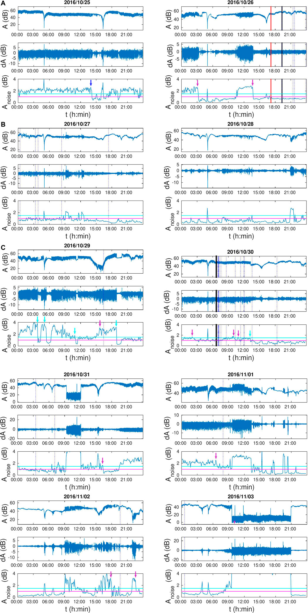
FIGURE 3. The time evolutions of the recorded amplitude A (A), its deviation, dA, from the base curve (B), and the noise amplitude, Anoise, (C) for the period of 25 October to 3 November 2016. Vertical lines indicate the times of earthquakes of magnitude 4 ≤ M < 5 (blue dot lines), 5 ≤ M < 6 (red line) and 6 ≤ M (black lines). Horizontal magenta and cyan lines indicate the amplitude of 1 and 1.5 dB, respectively. The beginnings of the amplitude noise reductions of Type I, II and III are indicated by the magenta, blue and cyan arrows, respectively.
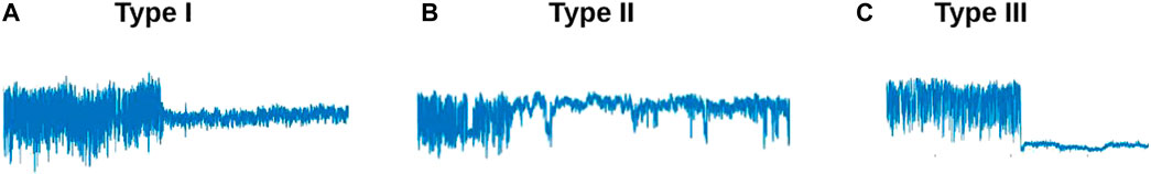
FIGURE 4. Display of the time evolution of the VLF signal amplitude A(t) during the amplitude noise reductions of Type I (A), Type II (B) and Type III (C).
The analysis of the presented parameters shows the following:
• 25 October. During this day, no strong EQs were recorded in the CI-1 area. A several-hour Anoise reduction that is visible in the afternoon corresponds to the time period around EQ of magnitude 3.9 in the CI-2 area. In other periods, the approximate value of Anoise is 2 dB, and it can be considered as Anoise in quiet conditions.
• 26–28 October. The expected values of Anoise under quiet conditions are visible at the beginning of 26 October. Its reduction to values below 1 dB begins a little after 3 UT, which is about 14 h before the first considered large EQ of magnitude 5.5. This reduction is followed by an increase of Anoise to values between 2 and 3 dB in a period of about 3 h starting at about 10:40 UT. After that, Anoise drops again back to values below 1 dB (at approximatively 13:40 UT). This second reduction starts about 3.5 h before the mentioned EQ at 17:10 UT. Both of these Anoise reductions are of Type I. However, in the case of the first one, no earthquakes were recorded near the considered signal propagation path, which open the question: Can more reduction of Anoise occur before a strong earthquake or more (relatively) strong earthquakes (in this case, EQs of magnitudes of 5.5 and 6.1 and 7 EQs of magnitudes of 4–4.7 in a period shorter than 11 h)? The values of Anoise continued to be low for the next 2 days. In that period, 5 EQs (of magnitudes of 4.2 (three events) and of 4.4 (two events) were recorded on October 27, while there were no earthquakes of magnitude greater than 4 on October 28. It is important to note here that there were no additional significant reductions that could be linked with the mentioned five EQs.
• 29–31 October. Anoise exceeds 2 dB at the beginning of 29 October and it is very unstable until about 20 UT. During that period, four reductions of Anoise below 1.5 dB (Type 3) that cannot be associated with EQs (not even those of magnitude less than 4) and one of Type 1 preceding EQ of magnitude 4.4 are visible. During the period of this reduction, a large number of less intense EQs were recorded. After 20 UT, Anoise is stabilized between 1.5 and 2 dB until around 14 UT on 30 October. During this time period, an EQ of magnitude 6.5 and 12 EQs of magnitude between 4 and 4.6 occurred. Before the strongest of them, an additional noise amplitude reduction of Type I is recorded. After it, two small additional reductions of Type I which can be connected with EQs are visible. They are followed by one long-lasting additional reduction of Type III, during which four more EQs of magnitudes between 4.2 and 4.9 (two on 30 October and two on 31 October) occurred. The connection of these five EQs with the mentioned reduction is not fully possible to harmonize with the expected possible connections based on the explanation of the previous cases and those given in Nina et al. (2020). Namely, increases in Anoise are expected after each of the first three EQs due to their lower intensity and several hours apart from the next one. However, a large number of weaker earthquakes occurred in this period and their impact on the considered signal should not be excluded a priori (the potential connection of weaker earthquakes with Anoise reductions is reported in Nina et al. (2020)).
• 1–3 November. Before the last three EQs in the observed period, Anoise is around 2 dB and higher for a certain period of time and, in all three cases, reductions of this parameter is visible (the first reduction is of Type 1, and the second two also correspond mostly to this type).
Based on the above analysis, one can conclude that the reduction of Anoise with the characteristics described in Nina et al. (2020) is recorded in the case of all three earthquakes of magnitudes over 5 (5.5, 6.1 and 6.5) (Cheloni et al., 2017; Galli et al., 2017). The earthquakes of magnitudes from 4 to 5 mostly (25 out of 28 cases) occurred after these 3 higher intensity earthquakes when Anoise is already reduced. In those cases, the additional observed reduction is either weakened or absent. In three cases when Anoise is around 2 dB or higher in the period before the change, visible reductions of Anoise are recorded. A corresponding reduction is also recorded before the magnitude 3.9 earthquake with the epicentre in the CI-2 area during the first analysed day (without stronger earthquakes in the CI-1 area). In other words, the obtained results indicate that the detectability of the noise amplitude reduction is reduced if its value is previously reduced due to the influence of other earlier EQ events. This conclusion opens up an additional question: Are signals with low noise amplitude suitable for analyses of its reduction as a potential precursor of earthquakes? In addition, the obtained results indicate the necessity to exclude the temporally close EQs from statistical analyses of effects of various parameters related to the characteristics of the analysed earthquakes, VLF signal and the environment in which it spreads to the noise amplitude reduction properties as such frequent EQs could simultaneously affect the signal.
The analysis of the connection between the Anoise reductions of the mentioned types and the occurrence of earthquakes whose magnitude is not less than 4 shows that the majority of Type I reductions (8 out of 10, i.e. 80%) and the only recorded Type II reduction are accompanied by observed phenomenon, which is in agreement with the study given in Nina et al. (2020). Although an earthquake was recorded after the Type III reduction on 30 October 2016, the previous analysis and the absence of that connection in the paper Nina et al. (2020) indicate that these phenomena are most likely not related.
In order to compare the presented analysis for PISA and periods without EQs, we additionally analyse the 6 days before and 6 days after those considered in this study. Based on the corresponding graphs and the detailed analysis given in the Supplementary Material, it can be seen that the reductions of all three types are also visible in these periods. However, out of a total of 18 reductions, 8 (4 of Type I, 3 of Type II and 1 of Type III) are in periods when the intensity of the amplitude is changed (e.g. in ST periods), 3 (all of Type III) are in the period of bad meteorological conditions, 1 (of Type II) in the period when the amplitude is unexpectedly low for the corresponding part of the day), while 4 (1 of Type I and 3 of Type II) have the same value as during most of the day but are preceded by short-term increases in Anoise. The only two Anoise reductions that have the properties of those described for PISA and in Nina et al. (2020) are reductions of Type III that, based on the previous analysis, cannot be considered as potential earthquake precursors.
The analysis presented in the previous section shows that the noise amplitude reductions can be clearly associated with the strongest earthquakes that occurred on 26 and 30 October, as well as the three earthquakes recorded from 1 to 3 November. In the following analysis we examine localization of the perturbations by processing two additional signal amplitudes in the case of the three strongest EQs, and during 27 October when no earthquake of magnitude greater than 5 was recorded. We consider the DHO and JYN signals that spread in the areas from their transmitters located in Germany and Norway, respectively, to the receiver in Belgrade. As one can see in Figure 1A the ICV signal propagation path is closest to the CI-1 area and it is located south of the seismic active zone. The paths of the other signals pass through areas north of the epicentres of the observed earthquakes.
The time evolutions of these signals for the mentioned 3 days are shown in Figure 5. In the case of the first day, the two noise amplitude reductions (for the ICV signal) associated in the previous Section with the EQs of magnitudes of 5.5 and 6.1 are visible in both reference signals. The Anoise reductions are almost twice smaller for the farthest signal from the CI-1 area (JXN) than for the ICV signal, while in the case of the DHO signal, the increase in Anoise between these reductions is significantly smaller than for the ICV signal, which decreases the intensity of the second reduction. In the case of the EQ of the 6.5 magnitude that occurred on 3 November, the Anoise reductions are similar for all signals, except that the least pronounced is the JYN signal, which, in addition to being the furthest from the seismically active area, also has the largest Anoise during quiet conditions.
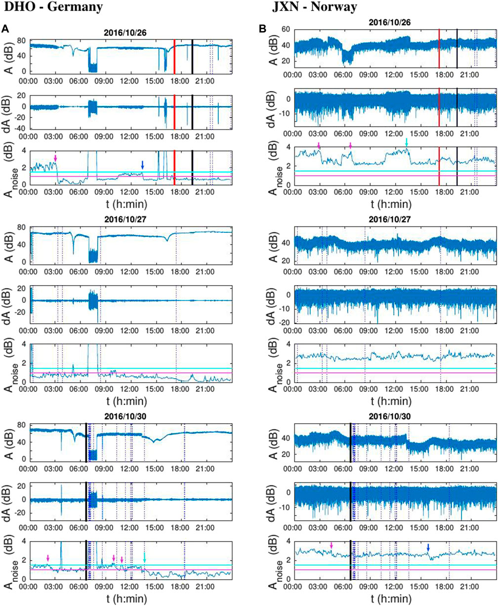
FIGURE 5. The time evolutions of the recorded amplitude A (upper panels), its deviation, dA, from the base curve (middle panels), and the sum amplitude, Anoise, (lower panels) for the DHO (A) and JXN (B) signal on 26 (upper panels), 27 (middle panels) and 30 (bottom panels) October 2016. Vertical lines indicate the times of earthquakes ofmagnitude 4 ≤M< 5 (blue dot lines), 5 ≤M< 6 (red line) and 6 ≤M(black lines). Horizontal magenta and cyan lines indicate the amplitude of 1 and 1.5 dB, respectively. The beginnings of the amplitude noise reductions of Type I, II and III are indicated by the magenta, blue and cyan arrows, respectively.
Based on this analysis, we can conclude that the Anoise reduction is visible in all three signals in the case of the strongest observed earthquakes. This indicates the possibility that the perturbed area has larger dimensions or that it is drifted closer to the receiver (in this way, more observed signals pass through a smaller area). Here it is important to point out that the existence of differences in the changes of Anoise, as well as the impossibility of establishing connections between their values, and the values of the signal amplitudes (e.g., the time evolutions of Anoise are similar for the ICV and DHO although the amplitude of the DHO signal is significantly higher than the other two) or Anoise (e.g., the difference in Anoise between the two reductions visible on 26 October between the DHO signal, and the ICV signal although their previous Anoise are very similar) are important for this study. Namely, they indicate that, although they are recorded for several signals, these changes are probably not the result of an unstable reception, but rather reflect variations of atmospheric parameters that can be spatially variable. This conclusion is supported by the difference in the time evolutions of the Anoise of the JXN signal from those of the other signals (first of all, the absence of the Anoise reduction at the end of October 27 in the case of the JXN signal, although they are similar for the remaining two signals), as well as the fact that the observed reductions occurred at different parts of the day when the same influence of man-made factors is not expected.
To examine the long-term variations of the signal amplitude, we analyse the time evolutions of noise amplitude characteristics on a daily basis for the time period from 1 October to 22 December (data for some days are missing due to absence of detection of the ICV signal by the AbsPAL receiver in Belgrade). Figure 6A shows the mean, median, minimum, and maximum noise amplitude values during day, as well as the corresponding standard deviation. The displayed values are obtained after eliminating the data during the period when either the signal was not detected by the AbsPAL receiver in Belgrade, or the noise amplitude is unusually high (indicating periods of solar terminators or the presence of some sudden disturbance). For the shown values, the criterion for this elimination is Anoise = 3 dB (this value is by 1 dB higher than Anoise in quiet conditions, which makes it possible to eliminate the consideration of perturbations that are a consequence of the mentioned causes which are not related to seismic processes). The essential influence of the choice of this value on the obtained conclusions is excluded by an additional check of the limiting values of 2.5 and 3.5 dB.
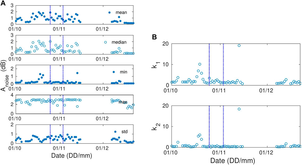
FIGURE 6. (A): the time evolutions of mean, median, minimum and maximum values of Anoise during the day and their standard deviations. (B): the ratio of the mean values and the standard deviation of Anoise labelled as k1 (upper panel), and the ratio of minimum values and standard deviation of Anoise labelled as k2 (bottom panel).
The obtained time evolutions of the observed parameters show the following:
• The mean and median values of Anoise start to increase on October 12 (13 days before PISA). The end point of this period cannot be exactly determined due to lack of data, but it is evident that from 7 December these values are reduced to those at the beginning of the shown period. In addition to the increases of the considered parameters, the dispersions of the displayed points are also increased in this period. Variations of the standard deviation of the Anoise values before PISA are more clearly defined, and its saturation is visible in the last considered week (later than the dependence of daily mean and median values of Anoise.
• The minimum values of Anoise are very similar during the entire observed time interval with clearly observed peaks at 5–8 days before and 10 days after PISA, respectively.
• The maximum values of Anoise are reduced at the beginning and end of the observed time interval as well as during 3 isolated days (1 during PISA and 2 after it).
• The times of the expressed peaks of the mean, median and minima of Anoise values before and after PISA correspond to the expressed minima of the standard deviation. This can be clearly seen in the form of pronounced maxima in the right panels in Figure 6 that show the time evolutions of the ratio of the mean values and the standard deviation of Anoise, indicated as k1 (upper panel), and the ratio of minimum values and standard deviation of Anoise indicated as k2 (lower panel).
The above conclusions point to changes in the daily characteristics of Anoise that begin about 2 weeks before PISA and end no later than about a month after PISA.
The presented analysis of the noise amplitude in a localized area during PISA is a pioneer study and the confirmation of the obtained conclusions requires additional case studies or statistical research which should be carried out in future. However, a comparison of the study of the VLF signal characteristics related to separated relatively strong EQs given in Nina et al. (2020) and Nina et al. (2021a) indicates similarities with conclusions obtained in this study for the corresponding periods. The potential horizontal displacements and enlargements of the area related to the seismic zone indicated in this study are also shown in the studies of the atmospheric chemical potential (ACP) and TEC. Although they refer to atmospheric areas near the surface and, primarily, in the upper ionosphere, respectively, their comparisons with variations in VLF signals propagating between Earth surface and the lower ionosphere are relevant because the seismo-ionospheric anomalies are not limited by some fixed altitude of the ionosphere but are continued to the upper altitudes into the magnetosphere forming the field-aligned irregularities of electron concentration (Pulinets et al., 2002). The physical nature of ACP, and the physical interfaces of the lithosphere-ionosphere coupling (generation of ACP) and atmosphere-ionosphere coupling (generation of TEC anomalies) are described in, for example, Pulinets et al. (2015a) and Pulinets et al. (2018b). The common agent of the link between the ACP and TEC are the complex ions formed in the process of the Ion Induced Nucleation (INN). The sharp (hyperbolic) growth of large complex ions concentration and their hydration leads to the growth of ACP. Simultaneously the same complex ions sharply decrease the conductivity of the atmospheric column between the ground and ionosphere increasing the ionospheric potential (IP) and formatting the positive anomalies of TEC. The physical mechanism of the seismo-ionospheric coupling and statistical proofs of connection of an earthquake with TEC variations is described in Pulinets and Boyarchuk (2004); Pulinets et al. (2015b); Pulinets et al. (2018); Liu et al. (2018). In addition, the observed diurnal changes exhibit some characteristics similar to those identified in many studies describing different types of ionospheric disturbances. In the following text, we point out these similarities and agreements.
As stated in Section 3.1.1, the Anoise reductions connected with the EQs that occurred during the period when the noise amplitude corresponds to that in quiet conditions have characteristics very similar to those shown in Nina et al. (2021b) for all EQs of magnitudes M ≥ 4 as well as for 9 EQs of magnitudes M ≤ 4.
Contrary to the results presented in Nina et al. (2021b) where the noise amplitude reductions are visible only for the ICV signal, the analysis performed in this study shows corresponding changes for several VLF signals. As stated in Section 3.1.2, this may be due to a larger area influenced by seismic activity or its drifting towards the location of the receiver. Both mentioned phenomena have already been presented in the literature (Biagi et al., 2012). The study presented in Sanchez-Dulcet et al. (2015) indicates a combination of both possibilities as well as the temporal variability of the spatial distribution of atmospheric disturbances. The larger perturbed area through which the considered VLF signals propagate is also consistent with the spatial distribution of ACP around the time of the Norcia M6.5 earthquake that occurred on 30 October 2016 (see Figure 7A). This parameter is the so-called integrated parameter actually been the proxy of the radon activity and its measurement at the 100 m altitude can be used for estimation od the disturbed area (Pulinets et al., 2015). The considered anomaly activity shown in this map covers (and exceeds) the whole region of Italian seismic activity during 2009–2017 presented in Soldati et al. (2020) (Soldati et al., 2020). Finally, the spatial distribution of TEC, presented in Figure 7B, shows a large disturbed area which includes the region around the receiver location.
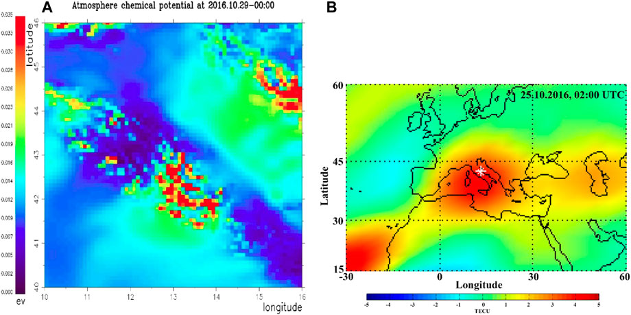
FIGURE 7. (A): Spatial distribution of ACP on 29 October 2016 at 00:00 UT. (B): The positive ionosphere anomaly detected over the area of the Norcia M6.5 earthquake preparation zone at 02:00 UTC. White cross – the epicentre position.
As stated in Introduction, studies in the literature primarily point to ionospheric variations that start a few days or several hours before major earthquakes. These variations apply to both the low and high ionosphere. Variations detected by VLF/LF signals occur in the form of the amplitude minimum time shift during solar terminator periods (the so-called “terminator time”) (Hayakawa, 1996; Molchanov et al., 1998; Yamauchi et al., 2007; Yoshida et al., 2008; Maurya et al., 2016), signal amplitude variations (Biagi et al., 2001a,b; Zhao et al., 2020), and periodic fluctuations (Miyaki et al., 2001; Molchanov et al., 2001; Rozhnoi et al., 2004; Biagi et al., 2006; Hayakawa et al., 2010; Ohya et al., 2018). These variations can be detected using different methods such as analyses of the standard deviation, the Wavelet spectra, the terminator time, deviations from mean values, and the Principal Component Analysis (Hayakawa, 1996; Biagi et al., 2012). Analyses of the GNSS signals indicate variation in TEC a few days before the considered EQ events. Examples of these changes can be seen in, for example, Pulinets and Davidenko (2018a) and Abdennasser and Abdelmansour (2019). In addition, it is found that the pre-seismic anomalies related to the acoustic-gravity waves, energetic particle burst in radiation belt, magnetic field, electron density, electron temperature and surface latent heat flux are recorded several days before EQs (see, for example, Sasmal et al. (2021); Chowdhury et al. (2022); Ghosh et al. (2022)).
The results obtained in this study are in agreement with those reported in the literature. Namely, as stated in Section 3.1.2, the beginnings of changes in the time evolution of the analysed parameters that describe the noise amplitude are visible about 2 weeks (increases in mean and median values of Anoise and dispersion of relevant points in plots of the corresponding time evolutions), a week (peaks of minimum values of Anoise, and values of parameters k1 and k2), and on the day of the beginning of PISA (increasing the dispersion of the standard deviation Anoise).
Based on the comparison mentioned inSections 3.3.1, 3.3.2, we can conclude that the presented analysis shows a confirmation of the previously presented variations of VLF signals, which are stated as possible precursors of earthquakes.
In this paper, we presented an analysis of VLF signal noise amplitude variations during the period of intense seismic activity in Central Italy from 25 October to 3 November 2016. It is a continuation of the study of possible connection between the noise amplitude reduction and earthquakes that can be analysed independently of other relevant connections due to a sufficiently large time interval between earthquake events and, in some cases, large spatial distances between their epicentres. In this study we analysed additional particular earthquake events and extended the global research to examination of a possible influence of the intense seismic activity to the observed signal characteristic changes. That was possible because we observed a time period when almost 1000 earthquakes (31 of them had a magnitude of 4 or greater, and the maximum magnitudes were 5.5, 6.1 and 6.5) were registered in a small area in Central Italy within only 10 days.
In this study we processed the amplitudes of the ICV, DHO and JXN signals emitted in Italy, Germany, the USA and Norway, respectively, and recorded in Belgrade, Serbia. The main analysis is performed for the ICV signal amplitude, while examination of other signal amplitude characteristics was done in order to analyse the localization of changes and possible variations in the noise amplitude due to problems in signal reception.
We presented analyses of: (1) the noise amplitude reduction which were first pointed out as potential precursors of earthquakes in the case of the Kraljevo earthquake that occurred in Serbia on 3 November 2010; (2) the daily characteristics of the VLF signal noise amplitude in the period from 1 October to 22 December, performed for the first time in this study.
Based on the results of the presented research, we can conclude the following facts:
• A significant reduction in the noise amplitude that can be associated with one or more earthquakes affects the possibility of detecting isolated significant reductions that can be associated with a particular earthquake.
• The noise amplitude reduction is recorded for all three earthquakes of magnitudes greater than 5, which is in agreement with the results shown for the earthquakes near Kraljevo, and the Tyrrhenian and Western Mediterranean Sea (presented in the first study that examines the considered correlations). It is important to emphasize that two of these three earthquakes occurred within about 2 h and can be related to the same reduction of the noise amplitude.
• Earthquakes of magnitudes between 4 and 5 that do not follow more intense earthquakes can also be connected with clear specific reductions in the noise amplitude, unlike those after more intense earthquakes for which additional reductions of already low noise amplitudes are small or completely absent.
• There are three types of the noise amplitude reduction depending on whether the noise amplitude reduction is a consequence of the increasing lower and/or decreasing higher amplitude values. Based on the analyses shown in this study and in Nina et al. (2020), correlations between these reductions and earthquakes can be established in cases of the increasing lower and decreasing higher amplitude values (Type I), or when the increase of the lower amplitude values is recorded (Type II). In the cases of decreasing higher amplitude values (Type III), an appropriate correlation with the occurrence of earthquakes was not established.
These conclusions indicate the importance of the noise amplitude value in quiet conditions for the detection of its reduction which can be potentially connected with an earthquake. In other words, the application of low noise amplitude signals for the detection of potential precursors of these natural disasters is questioned. In addition, this study opens more questions that require statistical studies. They relate to the possibility of more the noise amplitude reduction before a strong earthquake or more (relatively) strong earthquakes, increase the unperturbed area through which the VLF signals propagate during the long-term intensification of seismic activity (i.e. a large number of earthquakes in a relatively short period), displacement of the area under influence of the seismic activity relative to the seismically active area, and existence of changes in daily noise amplitude characteristics several days before the intensification of seismic activity (an increase in the noise amplitude mean and median values, clearly defined oscillations of its standard deviation followed by an increase in the dispersion of points in the graph of its time evolution at the beginning of the period of the earthquake series, the short-term (1 day to a few days) peaks of the ratio of the mean/minimum noise amplitude values and its standard deviation before and after the period of intense seismic activity, and the increase of its minimum values). Analyses of these issues should be the focus of future studies. In addition, due to the complexity of the analyzed connection caused by the possibility of the influence of a large number of parameters describing the earthquake, the VLF signal and the environment in which it spreads, it is necessary to carry out a larger number of studies in order to (if possible) define the criteria (in different conditions) for establishing a connection between the noise amplitude reductions and earthquake occurrences.
Here, we point out that analyses of the VLF signal characteristics are not sufficient to obtain the necessary information about localization (vertical and horizontal) of perturbed area. For this reason, it is necessary to do more studies based on different kinds of observation data so that theoretical analyses and models can be provided. This issue will be subject of future investigation, too.
At the end, we emphasize that the results of this, the second, study of examining the possibility that the noise amplitude reduction of VLF signals is a precursor of earthquakes contribute to the statistic that indicates that such a conclusion is quite realistic. Namely, as in the case of the first relevant study where the observed type of connection was recorded for all recorded earthquakes with magnitude greater than 4 and with epicentres close to the observed signal path (4 events), this analysis also shows that such a connection is detectable in all cases when there is no influence of other events (all 6 events including two events close in time which are connected with the same reduction). This confirmation gives even more importance to the continuation of the relevant research.
Requests for the VLF data used for analysis can be directed to the corresponding author. The other datasets used for this study can be found in http://www.emsc-csem.org/Earthquake/, https://eswd.eu/cgi-bin/eswd.cgi, https://www-app3.gfz-potsdam.de/kp_index/Kp_ap_Ap_SN_F107_since_1932.txt, https://hesperia.gsfc.nasa.gov/goes/goes_event_listings/.
Conceptualization, methodology, investigation, resources, formal analysis, writing—original draft, preparation, visualization, AN; Software, data curation, AN, SM, VČ, and MU; Validation, PB, SP, LP, GN, and MR; Writing—review and editing, all authors. All authors have read and agreed to the published version of the manuscript.
The authors acknowledge funding provided by the Institute of Physics Belgrade, the Astronomical Observatory (the contract 451-03-68/2020-14/200002) and the Geographical Institute “Jovan Cvijić” SASA through the grants by the Ministry of Education, Science, and Technological Development of the Republic of Serbia.
The Kilpisjarvi VLF data were supplied by the Sodankyla Geophysical Observatory, University of Oulu, Finland. For checking of the meteorological conditions we used information given on the European Severe Weather Database website. For checking of the geomagnetic conditions we used information provided by the Geomagnetic Observatory Niemegk, GFZ German Research Centre for Geosciences.
Author SM was employed by the company Novelic.
The remaining authors declare that the research was conducted in the absence of any commercial or financial relationships that could be construed as a potential conflict of interest.
All claims expressed in this article are solely those of the authors and do not necessarily represent those of their affiliated organizations, or those of the publisher, the editors and the reviewers. Any product that may be evaluated in this article, or claim that may be made by its manufacturer, is not guaranteed or endorsed by the publisher.
The Supplementary Material for this article can be found online at: https://www.frontiersin.org/articles/10.3389/fenvs.2022.1005575/full#supplementary-material
Abdennasser, T., and Abdelmansour, N. (2019). Geodetic contribution to predict the seismological activity of the Italian metropolis by the ionospheric variant of GPS_TEC. J. Atmos. Solar-Terrestrial Phys. 183, 1–10. doi:10.1016/j.jastp.2018.12.006
Ammar, A., and Ghalila, H. (2016). Ranking of sudden ionospheric disturbances by means of the duration of VLF perturbed signal in agreement with satellite X-ray flux classification. Acta Geophys. 64, 2794–2809. doi:10.1515/acgeo-2016-0114
Basak, T., and Chakrabarti, S. K. (2013). Effective recombination coefficient and solar zenith angle effects on low-latitude D-region ionosphere evaluated from vlf signal amplitude and its time delay during X-ray solar flares. Astrophys. Space Sci. 348, 315–326. doi:10.1007/s10509-013-1597-9
Biagi, P., Castellana, L., Maggipinto, T., Piccolo, R., Minafra, A., Ermini, A., et al. (2006). Lf radio anomalies revealed in Italy by the wavelet analysis: Possible preseismic effects during 1997–1998. Phys. Chem. Earth, Parts A/B/C 31, 403–408. doi:10.1016/j.pce.2005.10.001
Biagi, P. F., Maggipinto, T., Righetti, F., Loiacono, D., Schiavulli, L., Ligonzo, T., et al. (2011). The European VLF/LF radio network to search for earthquake precursors: Setting up and natural/man-made disturbances. Nat. Hazards Earth Syst. Sci. 11, 333–341. doi:10.5194/nhess-11-333-2011
Biagi, P. F., Piccolo, R., Ermini, A., Martellucci, S., Bellecci, C., Hayakawa, M., et al. (2001a). Disturbances in LF radio-signals as seismic precursors. Ann. Geophys. 44, 4. doi:10.4401/ag-3552
Biagi, P. F., Piccolo, R., Ermini, A., Martellucci, S., Bellecci, C., Hayakawa, M., et al. (2001b). Possible earthquake precursors revealed by LF radio signals. Nat. Hazards Earth Syst. Sci. 1, 99–104. doi:10.5194/nhess-1-99-2001
Biagi, P., Righetti, F., Maggipinto, T., Schiavulli, L., Ligonzo, T., Ermini, A., et al. (2012). Anomalies observed in VLF and LF radio signals on the occasion of the Western Turkey earthquake (Mw= 5.7. Int. J. Geosciences 19, 2011. doi:10.4236/ijg.2012.324086
Calais, E., and Minster, J. (1998). GPS, earthquakes, the ionosphere, and the space shuttle. Phys. Earth Planet. Interiors 105, 167–181. doi:10.1016/S0031-9201(97)00089-7
Chakrabarti, S. K., Sasmal, S., and Chakrabarti, S. (2010). Ionospheric anomaly due to seismic activities – part 2: Evidence from D-layer preparation and disappearance times. Nat. Hazards Earth Syst. Sci. 10, 1751–1757. doi:10.5194/nhess-10-1751-2010
Chakraborty, S., and Basak, T. (2020). Numerical analysis of electron density and response time delay during solar flares in mid-latitudinal lower ionosphere. Astrophys. Space Sci. 365, 184–189. doi:10.1007/s10509-020-03903-5
Cheloni, D., De Novellis, V., Albano, M., Antonioli, A., Anzidei, M., Atzori, S., et al. (2017). Geodetic model of the 2016 central Italy earthquake sequence inferred from InSAR and GPS data. Geophys. Res. Lett. 44, 6778–6787. doi:10.1002/2017GL073580
Chowdhury, S., Kundu, S., Ghosh, S., Hayakawa, M., Schekotov, A., Potirakis, S. M., et al. (2022). Direct and indirect evidence of pre-seismic electromagnetic emissions associated with two large earthquakes in Japan. Nat. Hazards (Dordr). 112, 2403–2432. doi:10.1007/s11069-022-05271-5
Davies, K., and Baker, D. M. (1965). Ionospheric effects observed around the time of the Alaskan earthquake of March 28, 1964. J. Geophys. Res. 70, 2251–2253. doi:10.1029/JZ070i009p02251
Fu, C.-C., Wang, P.-K., Lee, L.-C., Lin, C.-H., Chang, W.-Y., Giuliani, G., et al. (2015). Temporal variation of gamma rays as a possible precursor of earthquake in the longitudinal valley of eastern Taiwan. J. Asian Earth Sci. 114, 362–372. doi:10.1016/j.jseaes.2015.04.035
Galli, P., Castenetto, S., and Peronace, E. (2017). The macroseismic intensity distribution of the 30 october 2016 earthquake in central Italy (Mw6.6): Seismotectonic implications. Tectonics 36, 2179–2191. doi:10.1002/2017TC004583
Ghosh, S., Chowdhury, S., Kundu, S., Sasmal, S., Politis, D. Z., Potirakis, S. M., et al. (2022). Unusual surface latent heat flux variations and their critical dynamics revealed before strong earthquakes. Entropy 24 (1), 23. doi:10.3390/e24010023
Grubor, D. P., Šulić, D. M., and Žigman, V. (2008). Classification of X-ray solar flares regarding their effects on the lower ionosphere electron density profile. Ann. Geophys. 26, 1731–1740. doi:10.5194/angeo-26-1731-2008
Hayakawa, M., Horie, T., Muto, F., Kasahara, Y., Ohta, K., Liu, J.-Y., et al. (2010). Subionospheric VLF/LF probing of ionospheric perturbations associated with earthquakes: A possibility of earthquake prediction. SICE J. Control, Meas. Syst. Integration 3, 10–14. doi:10.9746/jcmsi.3.10
Hayakawa, M. (1996). The precursory signature effect of the kobe earthquake on VLF subionospheric signals. J. Comm. Res. Lab. 43, 169–180. doi:10.1109/ELMAGC.1997.617080
He, L., Wu, L., Heki, K., and Guo, C. (2022). The conjugated ionospheric anomalies preceding the 2011 Tohoku-Oki earthquake. Front. Earth Sci. (Lausanne). 10, 23. doi:10.3389/feart.2022.850078
Hegai, V., Kim, V., and Liu, J. (2006). The ionospheric effect of atmospheric gravity waves excited prior to strong earthquake. Adv. Space Res. 37, 653–659. doi:10.1016/j.asr.2004.12.049
Inan, U. S., Lehtinen, N. G., Moore, R. C., Hurley, K., Boggs, S., Smith, D. M., et al. (2007). Massive disturbance of the daytime lower ionosphere by the giant γ-ray flare from magnetar SGR 1806-20. Geophys. Res. Lett. 34, L08103. doi:10.1029/2006GL029145
Kolarski, A., Grubor, D., and Šulić, D. (2011). Diagnostics of the solar X-flare impact on lower ionosphere through seasons based on VLF-NAA signal recordings. Balt. Astron. 20, 591–595.
Korepanov, V., Hayakawa, M., Yampolski, Y., and Lizunov, G. (2009). AGW as a seismo-ionospheric coupling responsible agent. Phys. Chem. Earth, Parts A/B/C 34, 485–495. doi:10.1016/j.pce.2008.07.014
Leonard, R. S., Barnes, J., and Barnes, R. A. (1965). Observation of ionospheric disturbances following the Alaska earthquake. J. Geophys. Res. 70, 1250–1253. doi:10.1029/JZ070i005p01250
Liperovsky, V. A., Pokhotelov, O. A., Meister, C. V., and Liperovskaya, E. V. (2008). Physical models of coupling in the lithosphere-atmosphere-ionosphere system before earthquakes. Geomagn. Aeron. 48, 795–806. doi:10.1134/S0016793208060133
Liu, J.-Y., Hattori, K., and Chen, Y.-I. (2018). Application of total electron content derived from the global navigation satellite system for detecting earthquake precursors. Am. Geophys. Union (AGU)) 17, 305. doi:10.1002/9781119156949.ch17
Maekawa, S., Horie, T., Yamauchi, T., Sawaya, T., Ishikawa, M., Hayakawa, M., et al. (2006). A statistical study on the effect of earthquakes on the ionosphere, based on the subionospheric LF propagation data in Japan. Ann. Geophys. 24, 2219–2225. doi:10.5194/angeo-24-2219-2006
Matzka, J., Stolle, C., Yamazaki, Y., Bronkalla, O., and Morschhauser, A. (2021). The geomagnetic kp index and derived indices of geomagnetic activity. Space weather. 19, e2020SW002641. doi:10.1029/2020SW002641
Maurya, A. K., Venkatesham, K., Tiwari, P., Vijaykumar, K., Singh, R., Singh, A. K., et al. (2016). The 25 april 2015 Nepal earthquake: Investigation of precursor in vlf subionospheric signal. J. Geophys. Res. Space Phys. 121, 416. doi:10.1002/2016JA022721
Mitra A. P. (Editor) (1974). Ionospheric effects of solar flares (Dordrecht: Astrophysics and Space Science Library), 46.
Miyaki, K., Hayakawa, M., and Molchanov, O. (2001). “The role of gravity waves in the lithosphere - ionosphere coupling, as revealed from the subionospheric LF propagation data,” in Seismo electromagnetics: Lithosphere - atmosphere - ionosphere coupling” (Tokyo: TERRAPUB), 229–232.
Molchanov, O., Hayakawa, M., and Miyaki, K. (2001). VLF/LF sounding of the lower ionosphere to study the role of atmospheric oscillations in the lithosphere-ionosphere coupling. Adv. Polar Up. Atmos. Res. 15, 146–158.
Molchanov, O., Hayakawa, M., Oudoh, T., and Kawai, E. (1998). Precursory effects in the subionospheric vlf signals for the kobe earthquake. Phys. Earth Planet. Interiors 105, 239–248. doi:10.1016/S0031-9201(97)00095-2
Molina, C., Boudriki Semlali, B.-E., Park, H., and Camps, A. (2022). A preliminary study on ionospheric scintillation anomalies detected using gnss-r data from NASA CYGNSS mission as possible earthquake precursors. Remote Sens. 14, 2555. doi:10.3390/rs14112555
Němec, F., Santolík, O., and Parrot, M. (2009). Decrease of intensity of ELF/VLF waves observed in the upper ionosphere close to earthquakes: A statistical study. J. Geophys. Res. 114, 4. doi:10.1029/2008JA013972
Nina, A., Biagi, P. F., Mitrović, S. T., Pulinets, S., Nico, G., Radovanović, M., et al. (2021a). Reduction of the VLF signal phase noise before earthquakes. Atmosphere 12, 444. doi:10.3390/atmos12040444
Nina, A., Nico, G., Mitrović, S. T., Čadež, V. M., Milošević, I. R., Radovanović, M., et al. (2021b). Quiet ionospheric D-region (qiondr) model based on VLF/LF observations. Remote Sens. 13, 483. doi:10.3390/rs13030483
Nina, A., Pulinets, S., Biagi, P., Nico, G., Mitrović, S., Radovanović, M., et al. (2020). Variation in natural short-period ionospheric noise, and acoustic and gravity waves revealed by the amplitude analysis of a VLF radio signal on the occasion of the Kraljevo earthquake (mw = 5.4). Sci. Total Environ. 710, 136406. doi:10.1016/j.scitotenv.2019.136406
Nina, A., Simić, S., Srećković, V. A., and Popović, L. Č. (2015). Detection of short-term response of the low ionosphere on gamma ray bursts. Geophys. Res. Lett. 42, 8250–8261. doi:10.1002/2015GL065726
Ohya, H., Tsuchiya, F., Takishita, Y., Shinagawa, H., Nozaki, K., and Shiokawa, K. (2018). Periodic oscillations in the d region ionosphere after the 2011 tohoku earthquake using LF standard radio waves. J. Geophys. Res. Space Phys. 123, 5261–5270. doi:10.1029/2018JA025289
Oyama, K. I., Devi, M., Ryu, K., Chen, C. H., Liu, J. Y., Liu, H., et al. (2016). Modifications of the ionosphere prior to large earthquakes: Report from the ionosphere precursor study group. Geosci. Lett. 3, 6. doi:10.1186/s40562-016-0038-3
Perrone, L., De Santis, A., Abbattista, C., Alfonsi, L., Amoruso, L., Carbone, M., et al. (2018). Ionospheric anomalies detected by ionosonde and possibly related to crustal earthquakes in Greece. Ann. Geophys. 36, 361–371. doi:10.5194/angeo-36-361-2018
Pulinets, S. A., and Davidenko, D. V. (2018a). The nocturnal positive ionospheric anomaly of electron density as a short-term earthquake precursor and the possible physical mechanism of its formation. Geomagn. Aeron. 58, 559–570. doi:10.1134/s0016793218040126
Pulinets, S. A., Ouzounov, D. P., Karelin, A. V., and Davidenko, D. V. (2015a). Physical bases of the generation of short-term earthquake precursors: A complex model of ionization-induced geophysical processes in the lithosphere-atmosphere-ionosphere-magnetosphere system. Geomagn. Aeron. 55, 521–538. doi:10.1134/S0016793215040131
Pulinets, S. A., Ouzounov, D. P., Karelin, A. V., and Davidenko, D. V. (2015b). Physical bases of the generation of short-term earthquake precursors: A complex model of ionization-induced geophysical processes in the lithosphere-atmosphere-ionosphere-magnetosphere system. Geomagn. Aeron. 55, 521–538. doi:10.1134/S0016793215040131
Pulinets, S., Boyarchuk, K., Hegai, V., and Karelin, A. (2002). Conception and model of seismo-ionosphere-magnetosphere coupling. Tokyo: TERRAPUB, 353–361.
Pulinets, S., and Boyarchuk, K. (2004). Ionospheric precursor of earthquakes. Heidelberg, Germany): Springer.
Pulinets, S., Ouzounov, D., Karelin, A., and Boyarchuk, K. (2022). Earthquake precursors in the atmosphere and ionosphere: New concepts. Berlin, Heidelberg, Germany: Springer.
Pulinets, S., Ouzounov, D., Karelin, A., and Davidenko, D. (2018b). Lithosphere–atmosphere–ionosphere–magnetosphere coupling—a concept for pre-earthquake signals generation. America: American Geophysical Union AGU. 77–98. doi:10.1002/9781119156949.ch6
Pulinets, S., and Ouzounov, D. (2011). Lithosphere–atmosphere–ionosphere coupling (LAIC) model – An unified concept for earthquake precursors validation. J. Asian Earth Sci. 41, 371–382. doi:10.1016/j.jseaes.2010.03.005
Rozhnoi, A., Solovieva, M., Molchanov, O., and Hayakawa, M. (2004). Middle latitude lf (40 khz) phase variations associated with earthquakes for quiet and disturbed geomagnetic conditions. Phys. Chem. Earth, Parts A/B/C 29, 589–598. doi:10.1016/j.pce.2003.08.061
Sanchez-Dulcet, F., Rodríguez-Bouza, M., Silva, H. G., Herraiz, M., Bezzeghoud, M., and Biagi, P. F. (2015). Analysis of observations backing up the existence of VLF and ionospheric TEC anomalies before the Mw6.1 earthquake in Greece, January 26, 2014. Phys. Chem. Earth Parts A/B/C 85, 150–166. doi:10.1016/j.pce.2015.07.002
Sasmal, S., and Chakrabarti, S. K. (2009). Ionosperic anomaly due to seismic activities; part 1: Calibration of the VLF signal of VTX 18.2 kHz station from Kolkata and deviation during seismic events. Nat. Hazards Earth Syst. Sci. 9, 1403–1408. doi:10.5194/nhess-9-1403-2009
Sasmal, S., Chowdhury, S., Kundu, S., Politis, D. Z., Potirakis, S. M., Balasis, G., et al. (2021). Pre-seismic irregularities during the 2020 Samos (Greece) earthquake (M = 6.9) as investigated from multi-parameter approach by ground and space-based techniques. Atmosphere 12 (8), 1059. doi:10.3390/atmos12081059
Schmitter, E. D. (2013). Modeling solar flare induced lower ionosphere changes using VLF/LF transmitter amplitude and phase observations at a midlatitude site. Ann. Geophys. 31, 765–773. doi:10.5194/angeo-31-765-2013
Soldati, G., Cannelli, V., and Piersanti, A. (2020). Monitoring soil radon during the 2016–2017 central Italy sequence in light of seismicity. Sci. Rep. 10, 13137. doi:10.1038/s41598-020-69821-2
Sorokin, V., and Yashchenko, A. (1999). Disturbances of conductivity and electric field in the earth-ionosphere layer over an earthquake preparation focus. Geomagnetism Aeronomy 39, 228–234. doi:10.1023/A:1021549612290
Thomson, N. R., Rodger, C. J., and Clilverd, M. A. (2005). Large solar flares and their ionospheric D region enhancements. J. Geophys. Res. 110, A06306. doi:10.1029/2005JA011008
Wang, J., Huang, Q., Ma, Q., Chang, S., He, J., Wang, H., et al. (2020). Classification of VLF/LF lightning signals using sensors and deep learning methods. Sensors 20, 1030. doi:10.3390/s20041030
Xiong, P., Long, C., Zhou, H., Battiston, R., De Santis, A., Ouzounov, D., et al. (2021). Pre-earthquake ionospheric perturbation identification using cses data via transfer learning. Front. Environ. Sci. 9, 4. doi:10.3389/fenvs.2021.779255
Yamauchi, T., Maekawa, S., Horie, T., Hayakawa, M., and Soloviev, O. (2007). Subionospheric VLF/LF monitoring of ionospheric perturbations for the 2004 mid-niigata earthquake and their structure and dynamics. J. Atmos. Solar-Terrestrial Phys. 69, 793–802. doi:10.1016/j.jastp.2007.02.002
Yoshida, M., Yamauchi, T., Horie, T., and Hayakawa, M. (2008). On the generation mechanism of terminator times in subionospheric VLF/LF propagation and its possible application to seismogenic effects. Nat. Hazards Earth Syst. Sci. 8, 129–134. doi:10.5194/nhess-8-129-2008
Yuen, P. C., Weaver, P. F., Suzuki, R. K., and Furumoto, A. S. (1969). Continuous, traveling coupling between seismic waves and the ionosphere evident in May 1968 Japan earthquake data. J. Geophys. Res. 74, 2256–2264. doi:10.1029/JA074i009p02256
Zhao, S., Shen, X., Liao, L., Zhima, Z., Zhou, C., Wang, Z., et al. (2020). Investigation of precursors in VLF subionospheric signals related to strong earthquakes (M > 7) in western China and possible explanations 7) in western China and possible explanations. Remote Sens. 12, 3563. doi:10.3390/rs12213563
Keywords: earthquakes, earthquake precursor, VLF signal, noise amplitude, ionosphere, intense seismic activity
Citation: Nina A, Biagi PF, Pulinets S, Nico G, Mitrović ST, Čadež VM, Radovanović M, Urošev M and Popović LČ (2022) Variation in the VLF signal noise amplitude during the period of intense seismic activity in Central Italy from 25 October to 3 November 2016. Front. Environ. Sci. 10:1005575. doi: 10.3389/fenvs.2022.1005575
Received: 28 July 2022; Accepted: 06 September 2022;
Published: 29 September 2022.
Edited by:
Jing Luo, Northwest Institute of Eco-Environment and Resources (CAS), ChinaReviewed by:
Shufan Zhao, Ministry of Emergency Management, ChinaCopyright © 2022 Nina, Biagi, Pulinets, Nico, Mitrović, Čadež, Radovanović, Urošev and Popović. This is an open-access article distributed under the terms of the Creative Commons Attribution License (CC BY). The use, distribution or reproduction in other forums is permitted, provided the original author(s) and the copyright owner(s) are credited and that the original publication in this journal is cited, in accordance with accepted academic practice. No use, distribution or reproduction is permitted which does not comply with these terms.
*Correspondence: Aleksandra Nina, c2FuZHJhc3RAaXBiLmFjLnJz
Disclaimer: All claims expressed in this article are solely those of the authors and do not necessarily represent those of their affiliated organizations, or those of the publisher, the editors and the reviewers. Any product that may be evaluated in this article or claim that may be made by its manufacturer is not guaranteed or endorsed by the publisher.
Research integrity at Frontiers
Learn more about the work of our research integrity team to safeguard the quality of each article we publish.