Semi-Empirical Models for the Bidirectional Water-Leaving Radiance: An Analysis of a Turbid Inland Lake

When a precise quantitative analysis of satellite measurements over bodies of water is required, the bidirectional effects of water-leaving radiance must be considered. The bidirectional reflectance distribution function (BRDF) is used to estimate the directional dependency of the radiance. Previous research on BRDF has focused on oceanic waters; few studies on turbid inland waters have been conducted. In this article, using multi-angle MISR measurements, five semi-empirical BRDF models (MAG2002, Lee2004, Park-Ruddick 2005, Woerd-Pasterkamp2008, and Lee2011) were quantitatively compared, and an adaptive algorithm was proposed over a typical turbid inland lake, Taihu Lake, China. Our results reveal the following: 1) the Woerd-Pasterkamp2008 and Lee2011 models provide the best fits with correlation coefficients greater than 0.8; 2) when prior modeling parameters were used, the Lee2011 model was still the most accurate with RMSEs less than 1.1%, while the accuracy of the Woerd-Pasterkamp2008 model varied; and 3) the use of an adaptive algorithm including an empirical rule based on the ratio of $b_{\text{b}}/a$ improved the accuracy. The results provide a theoretical basis for BRDF models and BRDF effects over inland Case II waters. They also provide a priori knowledge for future studies on water constituents and the quantitative inversion of atmospheric parameters.

Introduction

The spectral radiance emerging from a natural body of water is not generally isotropic (Jerlov and Fukuda, 1960). It depends on the sun-sensor geometry as well as the optical properties and constituents of the water (Zhai et al., 2015; He et al., 2017). For the accurate estimation of spectral radiance, the angular effects of the water-leaving radiance must be considered. Most algorithms that attempt to retrieve the properties and constituents of water are based on in situ measurements of upwelling spectral radiance from a single viewing angle and toward the zenith (Gordon and Morel, 1983). It is common practice in ocean color remote sensing to relate the water-leaving radiance to a common geometry or account for the angular effects (Kwiatkowska et al., 2008). Moreover, satellite measurements vary in sun-sensor geometries. On the other hand, bidirectional reflectance of the water surface reveals essential information. It characterizes the optical properties of water (Twardowski and Tonizzo, 2018a; Twardowski and Tonizzo, 2018b) and serves as the boundary condition for the retrieval of aerosol properties (Gordon et al., 1997; Gatebe and King, 2016). The development of accurate bidirectional reflectance distribution function (BRDF) models is important for the quantitative analysis of water bodies and aerosols.

In previous years, research effort has developed the general idea that the variation of bidirectional reflectance can be modeled (Gordon, 1989a; Hirata et al., 2009). Research on the bidirectional effects of a water light field began with clear Case I waters, mainly oceanic waters. In such waters, the optical properties are mainly controlled by phytoplankton and the phase function is related to the concentration of chlorophyll-a (Loisel and Morel, 2001). The models were confirmed by measurements (Morel et al., 1995) and remote sensing data (Morel and Gentili, 1996). In turbid waters, however, the optical properties are more complex. Studies on the anisotropy of the Case II waters, especially coastal waters, have been conducted (Hlaing et al., 2012). Bidirectional reflectance distribution models were established with simulations in these studies. However, the study of BRDF over inland waters is still rare (Li et al., 2014).

BRDF models can be broadly divided into three categories: 1) physical models based on radiative transfer equations (Jin and Stamnes, 1994; Fell and Fischer, 2001) and Monte-Carlo simulations (Morel and Gentili, 1991); 2) semi-empirical models based on physical models and free parameters (Morel and Gentili, 1993; Albert and Mobley, 2003; Gege, 2004); and 3) empirical models based on statistical relationships (Morel, 2009). Physical models provide good physical interpretations and accurate simulations of bidirectional water-leaving radiance, but they are so complicated that they incur large computational costs. Empirical models are simpler than others; however, they are less representative, especially for waters quite different from the sample of origin. Perhaps, most importantly, they cannot explain the physical factor of BRDF in water. Compared with physical models and empirical models, semi-empirical models can give physical interpretations with reliable simulations at low computational costs. Therefore, these semi-empirical models are widely used in water color remote sensing algorithms (Gleason et al., 2012).

In this study, we identified the five popular semi-empirical BRDF models among the current models and used them to parameterize the bidirectional water-leaving radiance. Morel et al. developed a BRDF model (referred to below as MAG2002) to estimate the angular change in upwelling radiation based on simulation tables of a radiative transfer model (Morel et al., 2002). This is currently the standard model used for oceanic remote sensing observations. In addition, in recent years, several polynomial models have been proposed for different types of water, including those developed by Lee et al. (2004), Lee et al. (2011), Park and Ruddick (2005), and Vanderwoerd and Pasterkamp (2008). Some of these models have been used to compare different oceanic waters, including Case I waters and coastal Case II waters. However, validations and comparisons of these semi-empirical models over turbid inland waters are still rarely conducted. In addition, studies of these models essentially rely on numerical simulations and field measurements (Gleason et al., 2012; He et al., 2017). Field datasets are limited by the distribution of measurement sites. Multi-angle remote sensing data can help a lot in the application of these models.

Because of the complex optical characteristics of turbid inland waters, research on the properties of the bidirectional water-leaving radiance of lakes is insufficient. In this article, we selected the five popular semi-empirical BRDF models among the current models to parameterize the bidirectional water-leaving radiance. The different BRDF models of water-leaving radiance were analyzed based on MISR data collected from Taihu Lake, China. Taihu Lake is a typical turbid lake. We also proposed an adaptive and empirical algorithm based on the various performances of the models. The results provide a theoretical basis for models over lakes based on multi-angle remote sensing data and the correction of the angular effect of the radiance. Our study provides a priori knowledge that can be used in future research on the retrieval of the constituents of water and aerosol parameters.

This article is organized as follows: Materials and Methods introduces the materials and provides a brief description of the method used in the study. Results presents the results of the comparison. Discussion discusses the advantages and limitations, and also proposes an adaptive algorithm. Finally, the conclusions are given in Conclusion.

Materials and Methods

Database

Taihu Lake is located in the Yangtze River Delta and is China’s third largest fresh water lake. It covers an area of ∼2,300 square kilometers with an average depth of over 1.9 m (Zhang et al., 2019). The water in Taihu Lake is constantly turbid and eutrophic, with a large area of optically deep waters (Shi et al., 2018); it represents an environment that is very different from clear oceanic waters and turbid coastal waters. Therefore, Taihu Lake is ideal for research on turbid inland waters. Figure 1 illustrates the location of Taihu Lake.

FIGURE 1

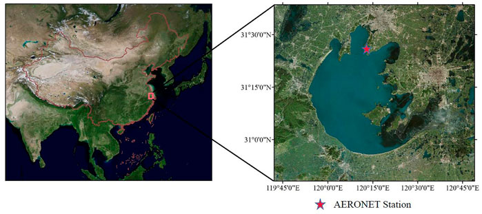
FIGURE 1. (A) Location of Lake Taihu in China; (B) location of the AERONET site on the northern edge of Lake Taihu.

The lake data used in this article came from the multi-angle database generated by MISR onboard the satellite platform Terra. As the MISR data now exceed over 20 years of global coverage, they provide a massive amount of directional reflectance information and having the advantage of accurate radiometric calibration. In addition to the nadir camera (AN), the forward and aft-viewing 26.1° cameras are called “AF” and “AA,” respectively, and those viewing at 45.6, 60.0, and 70.5° are noted as “B,” “C,” and “D,” respectively. The nine scans record observations in four spectral bands, with spatial sampling distances of 275 and 1,100 m. The center wavelengths are 446 nm (Blue Band), 558 nm (Green Band), 672 nm (Red Band), and 867 nm (NIR Band). The global repeat coverage time is between 2 and 9 days, depending on latitude. Observations for a single pixel are collected at 9 angles and taken within 7 min, meaning that the effect of dynamic inland water on the results is low. MISR is the only EOS series multi-angle instrument that can carry out long-term serial observations with a high level of spatial resolution and highly accurate radiometric calibration and stability (Si et al., 2021). The product of the radiance and geometric parameters can be used to analyze bidirectional reflectance. The MISR Level-2 surface product includes parameters of some bidirectional models, such as the hemispherical directional reflectance factor (HDRF) and bidirectional reflectance factor (BRF). These model parameters are not as accurate as expected due to the fitting errors. To reduce the error rate, the raw data used in this article are the MISR Level-1B products from 2015 to 2016. The MISR Level-1B product is top-of-atmosphere (TOA) reflectance. Based on the aerosol information from the AERONET site, we conducted atmospheric correction with the radiative transfer model of the coupled surface signals (Tanre et al., 1983) and the ASRVN (AERONET-based Surface Reflectance Validation Network) method (Yujie Wang et al., 2009). The accurate bidirectional reflectance data with atmospheric correction were used as a benchmark for the analysis in this study.

To improve the accuracy of atmospheric correction, we obtained precise aerosol data from the AERONET-Taihu Station. The AERONET (AErosol RObotic NETwork) program is a federation of ground-based remote sensing aerosol networks established by NASA and LOA-PHOTONS (CNRS). There is an observation site named Taihu Station on the north shore of Taihu Lake. Data from Taihu Station have been widely used in related scientific research. We downloaded aerosol data from this station and used them in the atmospheric correction process.

The inherent optical properties (IOPs) of pure seawater have known quantities (Morel, 1974; Pope and Fry, 1997), and the IOPs can be derived by the quasi-analytical algorithm (QAA) (Lee et al., 2011; Chen and Zhang, 2015). The series of QAA algorithms input the above-surface remote sensing reflectance and output IOPs of the absorption and backscattering coefficients. The measurements of IOPs from published datasets are sparse both in time and in space. The QAA-V algorithm (Joshi and D'Sa, 2018) was designed for use in the assessment of Case II waters and is suitable for MISR bands. Thus, we conducted QAA-V to get the absorption and backscattering coefficients of Lake Taihu.

To eliminate data on optically shallow waters, the MODIS SWIR and blue bands were obtained to distinguish waters. Morel’s oceanic models take wind into consideration. In this study, wind speed data for every six hours were obtained from global atmospheric reanalysis products provided by the National Centers for Environmental Prediction (NCEP).

BRDF Models of Water

A calm water body is a planetary surface with a unique BRDF pattern. In nature, we find large water bodies show anisotropy of the radiance field just above the water surface (Gatebe and King, 2016). We selected data from MISR observations made over Taihu Station and conducted accurate atmospheric corrections. Figure 2 illustrates the retrieved above-water remote sensing reflectance ($R_{\text{rs}}$) data plotted against scattering angles. Taihu Station was chosen as an example because of its stable water quality and sufficient level of aerosol products.

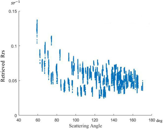
FIGURE 2

FIGURE 2. $R_{rs}$ retrieved over Taihu Station plotted against scattering angles.

The scattering angles in Figure 2 were calculated based on the following formula:

$\text{cos}\xi =\cos {\theta }_{\text{s}}\cos {\theta }_{\text{v}}+\sin {\theta }_{\text{s}}\sin {\theta }_{\text{v}}\sin \mathrm{\Delta }\varphi ,(1)$

where $\xi$ the scattering angle; ${\theta }_{\text{s}}$ and ${\theta }_{\text{v}}$ are the solar zenith angle and the view zenith angle, respectively; and $\Delta \varphi$ is the relative azimuth angle between the solar and view directions. We presented five semi-empirical BRDF models here. Table 1 lists the models and the related information.

TABLE 1

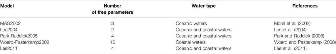
TABLE 1. Summary of BRDF models used to assess water.

MAG2002

Morel et al.’s (2002) model (referred to as MAG2002 in this article) is the standard model for oceanic remote sensing. It accounts for Raman scattering and the variance of particle phase function with respect to chlorophyll concentration. The MAG2002 model is a well-known model for oceanic waters and works well in studies conducted in clear oceanic areas (Voss et al., 2007). MAG2002 is widely used in correcting the angular measurements to be normalized water-leaving radiance, with both the solar zenith angle and view zenith angle of 0°. The applicability of the MAG2002 model in inland waters is worth studying and comparing with coastal models. The model is written as follows:

$R_{\text{rs}}({\theta }_{\text{s}},{\theta }_{\text{v}},\mathrm{\Delta }\phi ,\lambda ,W,\left[Chl\right])=\Re ({\theta }_{\text{v}},W)\times \frac{f}{Q}({\theta }_{\text{s}},{\theta }_{\text{v}},\mathrm{\Delta }\phi ,\lambda ,\left[Chl\right])\times \frac{b_{\text{b}}\left(\lambda \right)}{a\left(\lambda \right)},(2)$

where $R_{\text{rs}}$ is the above-water remote sensing reflectance; $\Re$ is a factor of cross-surface effects (Gordon, 2005) that can be obtained from a look-up table (LUT) published in the study by Morel and Gentili (1996); $f$ can be calculated using the solar zenith angle and the backscattering coefficient (Morel and Gentili, 1991); $Q$ is defined as the ratio of the upwelling irradiance to radiance; $a$ and $b_{\text{b}}$ are the IOPs of water, which represent the total absorption coefficient and total backscattering coefficient, respectively; $\lambda$ is the wavelength; $W$ is the wind speed obtained from the NCEP; and $\left[Chl\right]$ is the chlorophyll concentration.

Lee2004

Lee et al. (2004) proposed a model (referred to as the Lee2004 model in this article) for use over optically deep water. It is based on absorption and backscattering properties instead of chlorophyll concentration. The Lee2004 model explicitly expresses the remote sensing reflectance using two separate terms: one governed by the phase function of molecular scattering and the other governed by the phase function of particle scattering (Mobley, 1994). Model parameters have been developed for each term. The two-term formula is written as follows:

$r_{rs}(\lambda ,{\mathrm{\Omega }}^{\prime })=g_{\mathrm{w}}{\mathrm{(\Omega )}}^{\prime }\frac{b_{\mathrm{b}\mathrm{w}}\left(\lambda \right)}{a\left(\lambda \right)+b_{\mathrm{b}}\left(\lambda \right)}+g_{\mathrm{p}}(\lambda ,{\mathrm{\Omega }}^{\prime })\frac{b_{\mathrm{b}\mathrm{p}}\left(\lambda \right)}{a\left(\lambda \right)+b_{\mathrm{b}}\left(\lambda \right)},(3)$

where $r_{\text{rs}}$ is the subsurface remote sensing reflectance, defined by the ratio of upwelling radiance to downwelling irradiance just below the water surface; ${\Omega }^{\text{'}}$ is the sun-sensor angular geometry in the water; $b_{\text{bw}}$ and $b_{\text{bp}}$ are the backscattering coefficients of water molecules and particles, respectively; and $b_{\text{bw}}+b_{\text{bp}}=b_{\text{b}}$; $g_{\text{w}}$ and $g_{\text{p}}$ are two independent model parameters.

In order to keep the comparison consistent, we needed to convert $r_{\text{rs}}$ into $R_{\text{rs}}$. In studies on water color remote sensing, $r_{\text{rs}}$ and $R_{\text{rs}}$ have been related using the following formula (Lee et al., 2002; Sokoletsky and Shen, 2014):

$r_{\mathrm{r}\mathrm{s}}\left(\lambda \right)=R_{\mathrm{r}\mathrm{s}}\left(\lambda \right)/(1.7R_{\mathrm{r}\mathrm{s}}\left(\lambda \right)+0.52).(4)$

Park-Ruddick2005

Park and Ruddick (2005) used a 4th-order polynomial (their model is referred to as Park-Ruddick2005 here) to incorporate multiple-scattering effects for both Case I and Case II waters. The center of the high-order model is the ratio of backscattering ($b_{\text{b}}$) to the sum of absorption and backscattering coefficients ($a+b_{\text{b}}$). The fourth-order polynomial was chosen because the associated numerical error was much smaller than 10% in Park and Ruddick’s experiment. The function is written as follows:

$r_{\mathrm{r}\mathrm{s}}(\lambda ,{\mathrm{\Omega }}^{\prime })={\displaystyle \sum _{i=1}^4{g}_{\mathrm{i}}({\mathrm{\Omega }}^{\prime })(\frac{b_{\mathrm{bp}}(\lambda )}{a(\lambda )+b_{\mathrm{b}}(\lambda )}}{)}^i,(5)$

where $g_{\text{i}}$ (i = 1–4) are coefficients for the various sun-sensor angular geometries.

Woerd-Pasterkamp2008

Vanderwoerd and Pasterkamp (2008) used information from the IOPs in coastal waters to create an algorithm named HYDROPT to retrieve chlorophyll-a from satellite remote sensing images. In HYDROPT, a BRDF model (here referred to as Woerd-Pasterkamp2008) was proposed. This model includes a polynomial of the natural logarithm of total absorption and total scattering. The model can be applied with any definition of the specific inherent optical properties of chlorophyll-a, suspended particulate matter (SPM), and colored dissolved organic matter (CDOM). The model is written as follows:

$\ln \left[r_{\mathrm{r}\mathrm{s}}(\lambda ,{\Omega }^{\prime })\right]={\displaystyle \sum _{i=0}^3{{\displaystyle \sum _{j=0}^3{P}_{\mathrm{i}\mathrm{j}}{\left[\ln \left(a\left(\lambda \right)\right)\right]}^i\left[\ln \left(b\left(\lambda \right)\right)\right]}}^j},(6)$

where $P_{\text{ij}}$ (i = 0–3, j = 0–3) are fit coefficients for the combination of solar zenith, sensor zenith, and the relative azimuth.

Lee2011

Lee et al. (2011) improved their Lee2004 model based on many satellite measurements. With the objective of efficiently processing a large volume of satellite data while, at the same time, explicitly accounting for the different effects of molecular scattering and particle scattering, a second-order modified model (referred to as Lee2011 in this article) was proposed. The new model is similar to that presented as Eq. 3 and is written as follows:

$R_{rs}(\lambda ,\mathrm{\Omega })={\mathrm{(G}}_0^w\mathrm{(\Omega )}+G_1^w\mathrm{\Omega }\frac{b_{\mathrm{b}\mathrm{w}}\left(\lambda \right)}{a\left(\lambda \right)+b_b\left(\lambda \right)})\times \frac{b_{\mathrm{b}\mathrm{w}}\left(\lambda \right)}{a\left(\lambda \right)+b_b\left(\lambda \right)}+{\mathrm{(G}}_0^p\mathrm{(\Omega )}+G_1^p\mathrm{(\Omega )}\frac{b_{\mathrm{b}\mathrm{p}}\left(\lambda \right)}{a\left(\lambda \right)+b_{\mathrm{b}}\left(\lambda \right)})\times \frac{b_{\mathrm{b}\mathrm{p}}\left(\lambda \right)}{a\left(\lambda \right)+b_{\mathrm{b}}\left(\lambda \right)},(7)$

where $G_0^{\text{w}}$, $G_1^{\text{w}}$, $G_0^{\text{p}}$, and $G_1^{\text{p}}$ are coefficients that are dependent on the angular geometry; and $\Omega$ is the sun-sensor angular geometry above water.

Data Preprocessing

Considering the cloud coverage of MISR data and the quality of AERONET data, we selected 20 days with 180 images in our study. As there were thousands of pixels in every image and the adjacent pixels were similar, we sampled the data to lower the computational cost. We chose 1 pixel from every 10 pixels to conduct the experiment. The database of the bidirectional above-water reflectance was used to compare the performance of these five semi-empirical models. In order to conduct the experiment precisely and properly, we preprocessed the raw data.

Atmospheric Correction

Atmospheric correction is the key to the study. It is the first step toward remote sensing of water color. The radiative transfer equation of the coupled water-leaving signals can be expressed as follows (Tanre et al., 1983):

$R_{\text{TOA}}(\tau ,{\mu }_{\text{s}},{\mu }_{\text{v}},\mathrm{\Delta }\varphi )=R_{\text{atm}}(\tau ,{\mu }_{\text{s}},{\mu }_{\text{v}},\mathrm{\Delta }\varphi ),(8)$

$+e\frac{-\tau }{{\mu }_{\text{s}}}e\frac{-\tau }{{\mu }_{\text{v}}}{R}_{\text{rs}}({\mu }_{\text{s}},{\mu }_{\text{v}},\mathrm{\Delta }\varphi ),(\mathrm{a})$

$+e\frac{-\tau }{{\mu }_{\text{v}}}{t}_{\text{d}}(\tau ,{\mu }_{\text{s}})\overline{\rho }(\tau ,{\mu }_{\text{s}},{\mu }_{\text{v}},\mathrm{\Delta }\varphi ),(\mathrm{b})$

$+e\frac{-\tau }{{\mu }_{\text{s}}}{t}_{\text{d}}(\tau ,{\mu }_{\text{v}})\overline{\rho \prime }(\tau ,{\mu }_{\text{s}},{\mu }_{\text{v}},\mathrm{\Delta }\varphi ),(\mathrm{c})$

$+t_{\text{d}}(\tau ,{\mu }_{\text{s}})t_{\text{d}}(\tau ,{\mu }_{\text{v}})\overline{\overline{\rho }}+\frac{T(\tau ,{\mu }_{\text{s}})T(\tau ,{\mu }_{\text{v}})S\left(\tau \right){\overline{\overline{\rho }}}^2}{1-S\left(\tau \right)\overline{\overline{\rho }}},(\mathrm{d})$

where $R_{\text{TOA}}$ is the reflectance received at the top of the atmosphere (TOA); $R_{\text{atm}}$ is the radiation of solar radiation directly reaching the sensor after the process of atmospheric transmission; $T$ is the atmospheric transmittance; $S$ is the backscattering coefficient of the atmosphere; $\tau$ is the atmospheric optical thickness (AOT); ${\mu }_{\text{s}}$ and ${\mu }_{\text{v}}$ are the cosine of the solar zenith angle and the view zenith angle, respectively; $\overline{\rho }$, $\overline{\rho \text{'}}$, and $\overline{\overline{\rho }}$ are the coupling terms and can be defined as follows:

$\overline{\rho }(\tau ,{\mu }_s,{\mu }_v,\mathrm{\Delta }\varphi )=\frac{{\displaystyle {\int }_0^{2\pi }}{\displaystyle {\int }_0^1\mu L^{\downarrow }(\tau ,{\mu }_s,\mu ,\mathrm{\Delta }\varphi \prime )}{R}_{\text{rs}}(\mu ,{\mu }_v,\mathrm{\Delta }\varphi \prime -\mathrm{\Delta }\varphi )d\mu d\mathrm{\Delta }\varphi \prime }{{\displaystyle {\int }_0^{2\pi }}{\displaystyle {\int }_0^1\mu L^{\downarrow }(\tau ,{\mu }_s,\mu ,\mathrm{\Delta }\varphi \prime )d\mu d\mathrm{\Delta }\varphi \prime }},(9)$

$\overline{\rho \prime }(\tau ,{\mu }_s,{\mu }_v,\mathrm{\Delta }\varphi )=\overline{\rho }(\tau ,{\mu }_v,{\mu }_s,\mathrm{\Delta }\varphi ),(10)$

$\overline{\overline{\rho }}=\overline{\overline{\rho \prime }(\tau ,{\mu }_s,{\mu }_v,\mathrm{\Delta }\varphi )}\approx \frac{{\displaystyle {\int }_0^1}{\displaystyle {\int }_0^{2\pi }}{\displaystyle {\int }_0^1{R}_{\text{rs}}(\mu ,\mu \prime ,\mathrm{\Delta }\varphi )\mu \mu \prime d\mu \prime d\mu d\mathrm{\Delta }\varphi }}{{\displaystyle {\int }_0^1}{\displaystyle {\int }_0^{2\pi }}{\displaystyle {\int }_0^1\mu \mu \prime d\mu \prime d\mu d\mathrm{\Delta }\varphi }},(11)$

As Eq. 8 shows, the contribution of the target pixel to the signal at TOA can be divided into four terms: 1) the signal directly transmitted to the water surface and directly reflected back to the sensor, 2) the signal scattered by the atmosphere then directly reflected back to the sensor, 3) the signal directly transmitted to the target but scattered by the atmosphere on its way to the sensor, and 4) the signal having at least two interactions with the atmosphere and one with the target (Tanre et al., 1983).

The remote-sensing reflectance signal ($R_{\text{rs}}$) is the ratio of water-leaving radiance to the downwelling irradiance incident on the water surface. The test of glitter should be applied to all the cameras of MISR within 40 degree of the specular direction (Limbacher and Kahn, 2017). With the specular reflections removed by the glitter mask in the study by Limbacher and Kahn (2017), the data of $R_{\text{rs}}$ do not include the reflection effects at the air/water interface. In our study, the remote-sensing reflectance signals were atmospherically corrected to remove the atmospheric effects with Level 2.0 measurements of the AERONET Taihu site. The AERONET-based Surface Reflectance Validation Network (ASRVN) method is based on aerosol measurements and has been proven to be of high quality (Yujie Wang et al., 2009). When the sky over the lake is clear and without cloud cover, the distribution of aerosols can be regarded as nearly horizontally uniform, and the ASRVN algorithm can be used to obtain the bidirectional reflectance for Taihu Lake.

To test the accuracy of atmospheric correction, we obtained measurements from sampling points over Taihu Lake. We compared the in situ measurements and the nadir water-leaving radiance with the ASRVN method in similar sun-view geometry. The results are shown in Figure 3. The relative error is less than that of the usual atmospheric correction methods in previous studies (Pahlevan et al., 2021). Thus, we took the retrieved reflectance as an accurate benchmark for the following study.

FIGURE 3

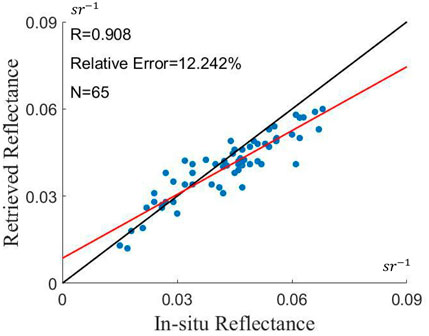
FIGURE 3. Comparison of in situ measurements and the retrieved reflectance at nadir view of MISR with the ASRVN method.

Water Types

Because bottom reflectance can significantly affect the bidirectional water-leaving radiance (Mobley et al., 2003), this study focused on optically deep waters where bottom reflectance is not an important factor. The first data processing step was to obtain the area of optically deep water. The extracted water areas were intersected with data contained in the Global Lakes and Wetland Database (GLWD) (Lehner and Döll, 2004). The reflectance of optically shallow water with a grass bottom is obviously higher than that of optically deep water in the SWIR band, and the sandy bottom will cause high reflectance in the Blue Band (Mobley–Curtis and Lydia, 2003). Therefore, to eliminate data on optically shallow waters, the MODIS SWIR and Blue bands were used to determine the threshold of the water-leaving radiance (Wang et al., 2018).

Studies have shown that the accuracy of the BRDF model is essentially related to the shape of the actual phase function of the water (Xiong et al., 2017). However, the phase function is scarcely measured because it is too complex for routine observations (Kirk, 1991). The absorption ($a$) and backscattering ($b_b$) coefficients are also widely used in the analysis and processing of water color data (Gordon, 1989b). In this article, we select IOPs of $a$ and $b_b$ as the main parameters to represent the water quality.

In order to compare the performance levels of models in different water types, we calculated the statistical numbers of sampled points with various IOPs. Based on the analysis of the IOPs and the previous research on long-term observations of Taihu Lake (Shi et al., 2019), we divided the data from Taihu Lake into five types. The range of IOPs and the statistical numbers of the sampled points in five water types are presented in Table 2.

TABLE 2

TABLE 2. Taihu Lake water types based on the IOPs at 558 nm (Green Band).

Data Experiments and Adaptive Algorithm

In our study, we conducted experiments based on Taihu Lake as a whole, as well as five different water types. We obtained bidirectional reflectance from MISR’s TOA measurements by atmospheric correction. The bidirectional data were used to compare the performance of five semi-empirical models. The method used for the comparison contained four parts: model fitting, modeling with prior parameters, difference comparison on scattering angles, and an adaptive algorithm.

For model fitting, the bidirectional reflectance is known, and models are inverted against the data for each target independently. Free parameters in this study are $Q$ in MAG2002, $g_{\text{w}}$ and $g_{\text{p}}$ in Lee 2004, $g_{\text{i}}$ (i = 1–4) in Park-Ruddick2005, $P_{\text{ij}}$ (i = 0–3, j = 0–3) in Woerd-Pasterkamp2008, and $G_0^{\text{w}}$, $G_1^{\text{w}}$, $G_0^{\text{p}}$, and $G_1^{\text{p}}$ in Lee 2011, respectively. For MAG2002, $Q$ is retrieved per water type and per sun-senor geometries. And for the other models, parameters are retrieved for every sun-senor geometry. Then these sets of free parameters are used to predict bidirectional reflectance. The optimization strategy for all the model fitting is least square minimization.

In most cases, however, bidirectional reflectance data are not available. Modeling with precomputed information is the usual way to figure out the accuracy of models and referred as prior parameters in our study. We selected data from 2015 as training data to obtain the parameters mentioned above. Then, we calculated the values of bidirectional reflectance based on the sun-view geometric data from 2016 and compared the simulations with the measurements.

The evaluation methods were the Pearson correlation coefficient (R), the root-mean-square error (RMSE), and the absolute relative error (ARE), which were calculated as follows:

$R=\frac{{\displaystyle {\sum }_{i=1}^n(xi-x)(yi-y)}}{\sqrt{{\displaystyle {\sum }_{i=1}^n{(xi-x)}^2{\displaystyle {\sum }_{i=1}^n{(yi-y)}^2}}}},(12)$

$RMSE=\sqrt{\frac{1}{\text{n}}{\displaystyle {\sum }_{i=1}^n{(R_{\text{rs}-\text{simulation}}-R_{\text{rs}-\text{measurement}})}^2}},(13)$

$ARE=\left|\frac{R_{\text{rs}-\text{simulation}}-R_{\text{rs}-\text{measurement}}}{R_{\text{rs}-\text{measurement}}}\times 100\%\right|,(14)$

Finally, we were trying to propose an adaptive algorithm for models to improve the accuracy in simulation. It was necessary to analyze the relationship between the models and the IOPs of $a$ and $b_{\text{b}}$. We took $b_{\text{b}}/a$ as the factor to represent the differences in water types in this study, because $b_{\text{b}}/a$ is a common ratio used in IOP studies of water color (Jerome et al., 1996; Twardowski and Tonizzo, 2018a). By analyzing the model’s performance against$b_{\text{b}}/a$, we figured a threshold to identify models’ performance. The adaptive algorithm was a modification of models. This algorithm could be applied for quantitative remote sensing over Taihu Lake, and its application could be expanded to other, similarly turbid lakes.

The flowchart is shown in Figure 4. The flowchart illustrates the four parts of our study.

FIGURE 4

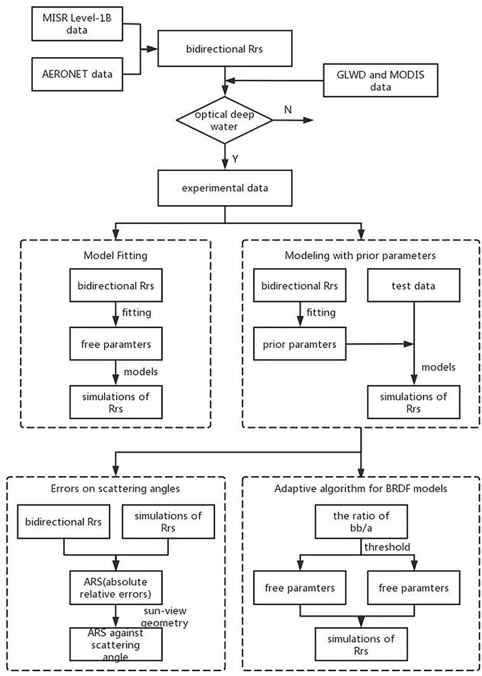
FIGURE 4. Flowchart of this study.

Results

Comparison for Model Fitting

The free parameters of the models were fitted from the retrieved bidirectional MISR data and then used to predict the $R_{\text{rs}}$. The scatter density plots were drawn from model simulations and measurements.

The scatter density plots in Figure 5 show the example of model simulations at the Green Band against measurements for the total lake. Accordingly, the plots in Figure 6 present the performances at the Green Band of the five types of water. Table 3 presents the detailed fitting result statistics for five models of four bands.

FIGURE 5

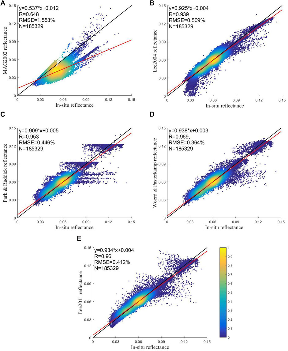
FIGURE 5. Scatter density plots of model simulations and measurements at the Green Band for Taihu Lake as a whole. The values are presented at linear scales. The solid red color lines in the figures are the fitting lines. The solid black lines are the reference lines of 1:1. The colors indicate the proportional number against the maximum of observations on the scale. The linear fitting formula (y), the correlation coefficient (R), the root-mean-square error (RMSE), and the number of measurements (N) are displayed on the upper left section of each plot.

FIGURE 6

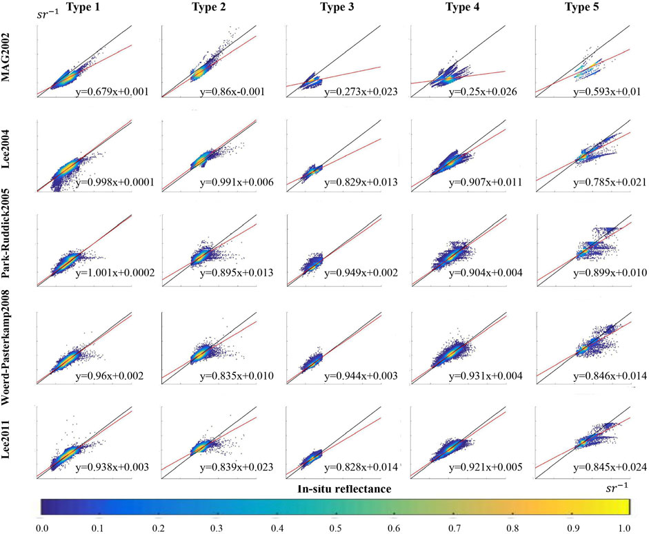
FIGURE 6. Scatter density plots of five model simulations and measurements conducted at the Green Band for five water types. The values are presented at linear scales. The solid red color lines in the figures are the fitting lines. The solid black lines are the reference lines of 1:1. The ranges of x-axis and y-axis are both 0–0.15.

TABLE 3

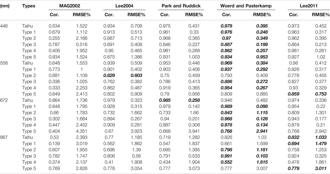
TABLE 3. Fitting result statistics for five models for Taihu Lake as a whole and for five water types. The bold-italic values mean the best results in every case.

Figures 5, 6 show a discontinuous distribution with some point split. For Taihu Lake as a whole, the performance of the models varied among bands. At the Blue Band (446 nm), the top models were Woerd-Pasterkamp2008, Park-Ruddick2005, and Lee2011. At the Green Band (558 nm), the best models were Woerd-Pasterkamp2008 and Lee2011. At the Red Band (672 nm), the Park-Ruddick2005 and Lee2011 models provided the best fits. The accuracy level for the NIR Band (867 nm) was lower than that for the other bands. MAG2002 was identified as the worst model for all bands, with simulated values being lower than the measured ones.

As for the various types of water, Woerd-Pasterkamp2008 was the model that provided the best fit for the Blue and Red Bands. It was the best for three types of water at the Green and NIR Bands. The Lee2011 model was the most successful for use in Type 1 waters at 872 nm and Type 5 waters at Green and NIR Bands. Lee2004 fit best in Type 2 waters at the Green Band.

Comparison for Modeling With Prior Parameters

The scatter density plots presented in Figure 7 show model simulations with prior modeling parameters at the Green Band versus measurements obtained for the lake as a whole. Detailed statistical data from all bands are listed in Table 4.

FIGURE 7

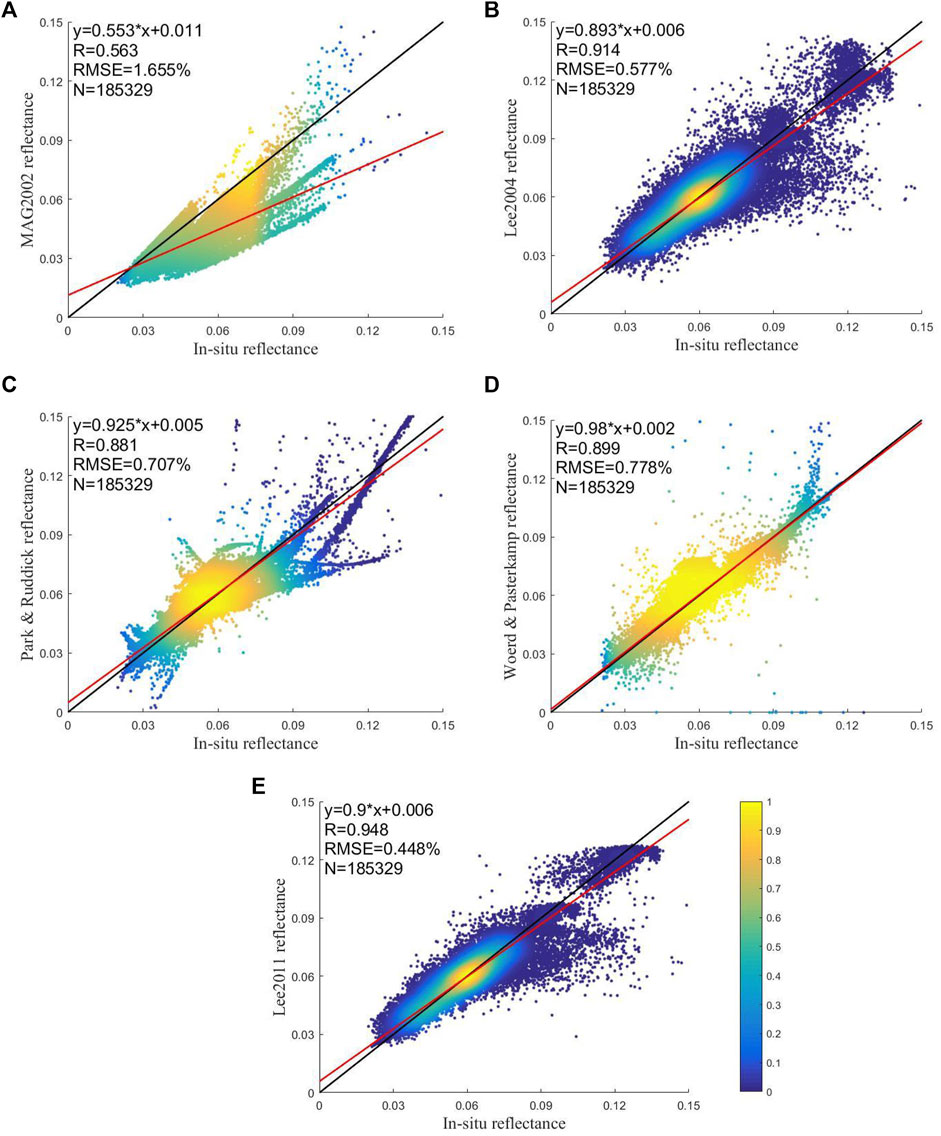
FIGURE 7. Scatter density plots to compare model simulations and measurements at the Green Band for Taihu Lake as a whole. The values are presented at linear scales. The solid red color lines in the figures are the fitting lines. The solid black lines are the reference lines of 1:1. The colors indicate the proportional number against the maximum of observations on the scale. The linear fitting formula (y), the correlation coefficient (R), the root-mean-square error (RMSE), and the number of measurements (N) are displayed on the upper left section of each plot.

TABLE 4

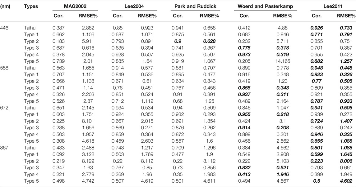
TABLE 4. Statistical data for the five models with prior parameters for Taihu Lake as a whole and for the five water types. The bold-italic values mean the best results in every case.

For Taihu Lake as a whole, the model performance varied among bands. At the Blue Band (446 nm), the top models were Park-Ruddick2005 and Lee2011. At the Green Band (558 nm), the best model was Lee2011. At the Red Band (672 nm), the Lee2011 and Park-Ruddick2005 models had the best fits. At the NIR Band (867 nm), Lee2011 was the most precise model. MAG2002 was the worst model for all bands. As for the various types of water, Lee2011 was the most accurate 11 times, followed by Woerd-Pasterkamp2008 with 8 times and Park-Ruddick2005 with 1 time.

Difference Comparison on Scattering Angles

To evaluate the overall performance of these BRDF models in the remote sensing domain (${\theta }_v$ = 0–71°) (Lee et al., 2011), we compared the accuracy with various sun-view geometries of MISR to show the angular deviations. According to the Comparison for Model Fitting and Comparison for Modeling With Prior Parameters, MAG2002 is not suitable for the inland lake, and error analysis of angular effects is focused on the inherent-optical-property-centered models (Lee2004, Park-Ruddick2005, Woerd-Pasterkamp2008, and Lee2011). Precomputed parameters are much useful in simulation and angular correction when the bidirectional measurements available are not sufficient. We applied these prior parameters to simulate bidirectional reflectance in many cases. Thus, we present the results of the models in Comparison for Modeling With Prior Parameters against scattering angles. The absolute relative differences are calculated based on ARE in Eq. 14. Figure 8 shows the scatter density plots of the absolute relative difference of five models against scattering angles.

FIGURE 8

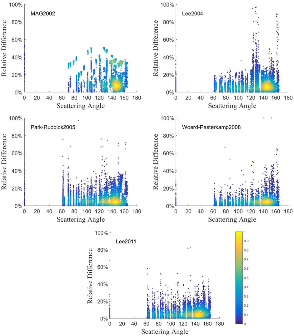
FIGURE 8. Scatter density plots of the absolute relative difference of five models against scattering angles.

As shown in Figure 8, Woerd-Pasterkamp2008 and Lee2011 are better than Lee2004 and Park-Ruddick2005. Woerd-Pasterkamp2008 is best when the scattering angle is less than 130°, but the absolute relative difference increases at large scattering angle. Lee2011 is excellent in the domain of scattering angle. The relative difference is less than 20% in most cases.

Adaptive Algorithm for BRDF Models

To illustrate the IOP effects explicitly, $R_{\text{rs}}$ of five water types at AN view (the nadir camera of MISR) was presented. The average of $R_{\text{rs}}$ at AN view is denoted as ${\left[R_{\text{rs}}\right]}_{\text{AN}}$ and shown in Figure 9.

FIGURE 9

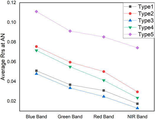
FIGURE 9. Average of $R_{\text{rs}}$ values at AN view of five water types drawn with four bands of MISR.

The various values of ${\left[R_{\text{rs}}\right]}_{\text{AN}}$ in five water types show that the backscattering coefficient has a greater influence than absorption coefficient. In addition to Woerd-Pasterkamp2008’s typical performance related to water types in Comparison for Modeling with Prior Parameters, we selected $b_{\text{b}}/a$ as a factor to compare models. Lee2011 was the best model according to the results. We compare Lee2011 and Woerd-Pasterkamp2008 against $b_{\text{b}}/a$ here to develop our adaptive algorithm.

Figure 10 illustrates that the correlation coefficient and RMSE of the two models when the $b_{\text{b}}/a$ of 1.1 at the Green Band were set as the threshold. When $b_{\text{b}}/a$ < 1.1 at the Green Band, the two models performed well. Woerd-Pasterkamp2008 was found to have a slight advantage and was more stable than Lee2011. When $b_{\text{b}}/a$ > 1.1 at the Green Band, however, the accuracy of Lee2011 was much better than that of Woerd-Pasterkamp2008.

FIGURE 10

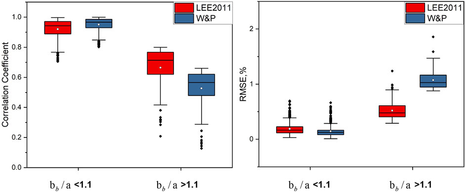
FIGURE 10. Boxplots of the correlation coefficient and RMSE values at the Green Band for Lee2011 and Woerd-Pasterkamp2008 in two groups of water.

Then we can manage a crossover method as the adaptive algorithm. The threshold of $b_{\text{b}}/a$ was set as 1.1, and the corresponding model was conducted. The results for the adaptive algorithm compared to Woerd-Pasterkamp2008 and Lee2011 models are shown in Figure 11.

FIGURE 11

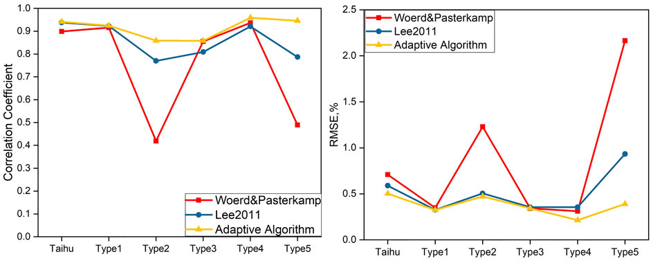
FIGURE 11. RMSE values and correlation coefficients of measurements and simulations conducted at the Green Band.

For the adaptive algorithm, the correlation coefficients were greater than 0.85 for all water types, while the RMSE values were lower than 0.5. Compared with the original models, the adaptive algorithm was found to be unquestionably more robust for simulating water-leaving radiance, especially in Type 2 and Type 5 waters. The adaptive algorithm is a modification of the top two models.

Discussion

Discussion of the Results

For the results presented in Results, one of the most obvious characteristics shown in the figures is that the plotted points are not continuous. This discontinuity is related to the discrete parameters based on the grid of sun-sensor geometries. The view zenith angles of MISR are quite sparse. The relative azimuth angles are not as different as the zenith angles over Taihu Lake. Thus, the sun-sensor angular geometries gather in clusters. The model parameters are fitted to the nearest geometry, and the sun-sensor geometries are not continuous. Thus, they are not as smooth as in the simulation based on a continuous sun-sensor geometry.

The model fitting comparison allowed us to determine the models with the best fit. Woerd-Pasterkamp2008 and Lee2011 had correlation coefficients greater than 0.8, showing almost unbiased comparisons and indicating that they are good fits for the shape of BRDF. For Taihu Lake as a whole, Woerd-Pasterkamp2008 provided the smallest RMSE values and the largest correlation coefficients at the Blue and Green Bands, while it was the second best model at the NIR Band and the third best model at the Red Band. Lee2011 was consistently one of the top models for all bands. The next best models were Park-Ruddick2005 and Lee2004. As for the various types of water, Woerd-Pasterkamp2008 was the best fitting model. It had the smallest RMSE value and the largest correlation coefficient in most situations. The Lee2011 model was the second best followed by Park-Ruddick2005 and Lee2004. MAG2002 was the worst model for all water types. These results are consistent with those obtained for Taihu Lake as a whole. The MAG2002 was identified as the worst model in all situations.

In the comparison with modeling using prior parameters, the rank of models changed. The accuracy of the models when a priori knowledge was used was lower than that obtained with model fitting. For Taihu Lake, as a whole, the best model was obviously Lee2011, which was identified as one of the top models for all bands. The next best model was Park-Ruddick2005, which was one of the best at the Blue and Red Bands. For the various types of waters, Lee2011 was the best overall. The next best models were Park-Ruddick2005 and Lee2004. Woerd-Pasterkamp2008 was less stable in terms of its precision and accuracy than the other models. MAG2002 was still the worst.

As for the various water types, the accuracy of model fitting varied widely. For example, the difference in correlation coefficients reached 0.6 for the MAG2002 model. However, clearly, all models except MAG2002 were more successful in water types where the effects of absorption and backscattering were similar. There were great differences in Woerd-Pasterkamp2008’s performance among the various water types. Woerd-Pasterkamp2008 performed the best for two water types (Types 3 and 4) and the worst for two water types (Types 2 and 5).

Apart from MAG2002, the main structure of the models had an inherent optical property center and parameters with a sun-view geometry. IOPs are the center of these four models, and they have various levels of sensitivity on the scattering angle.

Combined with the relative errors against scattering angle presented in Difference Comparison on Scattering Angles, the relative errors of four models are mainly less than 40%. Moreover, Lee2011 is stable in all the geometries, while Woerd-Pasterkamp2008’s errors increase at large scattering angles. Woerd-Pasterkamp2008 and Lee2011 are better, with relative errors less than 20%. These two models are suitable for all the remote sensing domains.

In a theoretical sensitivity study, Lee2011 proves its robustness with outstanding relative errors. Lee2004 is not sensitive to the absorption coefficient, but it is less robust to the backscattering coefficient. Park-Ruddick2005 is affected by IOPs. Woerd-Pasterkamp2008 is largely sensitive to IOPs, especially backscattering coefficients. Besides, the average ${\left[R_{\text{rs}}\right]}_{\text{AN}}$ in five water types shows that the backscattering coefficient has a greater influence than the absorption coefficient. Thus, an adaptive algorithm was proposed based on $b_{\text{b}}/a$ by applying various models in water. Lee2011 and Woerd and Pasterkamp are the top two models mentioned in previous results. In Type 3, where the effects of absorption are larger than those of backscattering, Woerd and Pasterkamp behave better than Lee2011. In Types 2 and 5, however, where the effects of absorption are less than those of backscattering, Lee2011 is more accurate than Woerd and Pasterkamp. Meanwhile, in Types 1 and 4, where the effects of absorption and backscattering are similar, the two models perform similarly. The adaptive algorithm improves the accuracy of BRDF simulations and expands the applicability of the models. When the uncertainty of the model is less than 10%, the model is acceptable for use in BRDF modeling and for the correction of bidirectional variation (Loisel and Morel, 2001).

Advantages and Limitations of the Models

MAG2002 is the standard oceanic BRDF model, but it performed badly in the Taihu Lake simulation. There are at least three reasons for this. First, because the model is based on Case I assumptions (Morel and Prieur, 1977), it requires the absorption contribution to co-vary with the concentration of chlorophyll-a (Morel and Maritorena, 2001) and ignores the other optically active factors in Case II waters, such as CDOM, SPM, and higher chlorophyll concentrations (Gleason et al., 2012). The second reason is the form of the model itself. Morel and Gentili parameterized $f$ and $Q$ as the function of the chlorophyll concentration in Case I waters. These parameters can be obtained from the previous LUT (Morel and Gentili, 1996) or calculated based on sun-sensor geometry, causing errors to accumulate. Another possible reason is the QAA-V process in this study. The structure of QAA-V is similar to the other models, and that might reduce the errors for the others. But we think the effects relating to the difference are less than the quality of models in turbid lakes. In fact, Park-Ruddick2005 is the most similar model to the structure of the QAA-V, but it is not the best model in our study. Thus, both theoretically and empirically, the MAG2002 model is not suitable for the quantitative analysis of inland Case II waters.

As for the other four models, one of the common characteristics is that they are inherent-optical-property-centered models and ignore inelastic scattering [like Raman scattering (Stavn and Weidemann, 1988; Hu and Voss, 1997) and chlorophyll-a fluorescence, which has an isotropic angular distribution (Gordon et al., 1993)]. This differs from MAG2002. Thus, all of these models can be applied for the analysis of the turbid inland waters. However, they vary in terms of their complexity and accuracy.

Park-Ruddick2005 performs well according to our results, but its level of uncertainty is much larger than that presented in Park and Ruddick’s experiments. According to Park and Ruddick’s research, the model’s uncertainty arises mainly from the phase function uncertainty and is generally less than 2%. This function can be applied to a wide range of $b_{\text{b}}/�a+b_{\text{b}}�$ values, but it is sensitive to the backscattering coefficient. In extremely turbid water, variations in the sensor zenith angle are significant (Park and Ruddick, 2005). In simulations, the sensor zenith angle is approximated to the nearest angle. This might be the main limitation of Park-Ruddick2005.

The fundamental difference between Lee’s models (Lee2004 and Lee2011) and the other models is that they account for molecular and particle backscattering separately. This feature works well in our simulation. We observed that Lee’s models were more stable in various water types than the Park-Ruddick2005 and Woerd-Pasterkamp2008 models. For Lee2011, another notable improvement is that the water-leaving radiance is simulated using linear mixing of the Petzold average particle phase function (Mobley, 1994), where mineral particles and the Fournier-Forand phase function (Fournier and Forand, 1994) are represented with a backscattering ratio of 1% (Mobley et al., 2002) to represent phytoplankton particles. The model is more robust and precise when used to assess turbid lakes than Lee2004 due to the new form of the model and the modified phase function.

The Woerd-Pasterkamp2008 model has the most free parameters and the highest order polynomial of natural logarithm. Its structure resulted in an exponential relative error in the sensitivity study. It was found to be the best model for model fitting. However, it performed badly when modeling with prior parameters. Notably, the model’s performance varied among water types. Woerd-Pasterkamp2008 had the worst performance for two water types (Types 2 and 5) where the effect of backscattering was larger than that of absorption. Conversely, it performed the best in the two water types (Type 3 and 4), where the effects of backscattering and absorption were similar. We will discuss this further in the following section.

We used Taihu Lake as an example of a turbid inland lake. In order to enhance the results for various water qualities, we divided the lake into five types (presented in Data Preprocessing) and applied the algorithm for their analysis. This algorithm can be applied for quantitative remote sensing over Taihu Lake, and its application can be expanded to other, similarly turbid inland waters.

Conclusion

In previous years, several BRDF models have been developed to parameterize the bidirectional water-leaving radiance of water surfaces. Although some achievements have been made through the comparison and validation of some of these models over clear oceanic Case I waters and coastal Case II waters, studies on turbid inland waters are lacking. We quantitatively compared the five popular models using a typical turbid inland lake, Taihu Lake, China, in this study.

Using a bidirectional reflectance database generated from space-borne MISR measurements, the model fitting accuracy of five models and the accuracy when prior modeling parameters were used were analyzed over Taihu Lake. The water was divided into five types based on IOPs in order to more accurately assess the performance of the models at various levels of water quality. The results suggest that Woerd-Pasterkamp2008 has the best fitting effects, followed by Lee2011. Based on the inappropriate hypothesis of the algorithm and phase function, MAG2002 was found to be unsuitable. On the other hand, when the prior parameters were used, Lee2011 was the most accurate and robust model for most water types. Woerd-Pasterkamp2008 behaved differently in terms of the ratio of IOPs $b_{\text{b}}/a$. Furthermore, the error comparison on scattering angles showed that Lee2011 and Woerd-Pasterkamp2008 were robust in the remote sensing domain. We identified a certain rule governing the relationship between model simulations and the ${\text{b}}_{\text{b}}/a$ ratio, which could be applied to obtain an adaptive algorithm. Based on this rule, we proposed an adaptive algorithm using the top two models to enhance their applicability. The algorithm improves the robustness and accuracy of bidirectional water-leaving radiance simulations.

In this article, we carried out a bidirectional reflectance model analysis of a typical turbid inland lake, Taihu Lake, in China. These results are important for the application of multi-angle remote sensing data and the correction of the BRDF effect of radiance. This research also provides a theoretical basis for future studies on the quantitative inversion of water constituents and surface atmospheric parameters over turbid lakes.

Data Availability Statement

The original contributions presented in the study are included in the article/Supplementary Material; further inquiries can be directed to the corresponding author.

Author Contributions

ZH and KB contributed to conceptualization; ZH and SS contributed to methodology; ZH and XZ contributed to software; ZH contributed to validation, formal analysis, investigation, data curation, writing—original draft preparation, visualization, and supervision; ZH and XG contributed to resources; ZH and SS contributed to writing—review and editing; ZH and XG contributed to project administration; SS and XG contributed to funding acquisition.

Funding

This research was funded by the National Key Research and Development Program of China (Grant Number: 2020YFE0200700) and the Natural Science Foundation of China (Grant Number: 42005104).

Conflict of Interest

The authors declare that the research was conducted in the absence of any commercial or financial relationships that could be construed as a potential conflict of interest.

Publisher’s Note

All claims expressed in this article are solely those of the authors and do not necessarily represent those of their affiliated organizations, or those of the publisher, the editors, and the reviewers. Any product that may be evaluated in this article, or claim that may be made by its manufacturer, is not guaranteed or endorsed by the publisher.

Acknowledgments

We would like to thank NASA for processing the MISR data and MODIS data, and we also thank NCEP for providing global atmospheric reanalysis products. We appreciate the PI investigators from the AERONET site, whose data were used in this article.

References

Albert, A., and Mobley, C. (2003). An Analytical Model for Subsurface Irradiance and Remote Sensing Reflectance in Deep and Shallow Case-2 Waters. Opt. Express 11, 2873–2890. doi:10.1364/oe.11.002873

PubMed Abstract | CrossRef Full Text | Google Scholar

Chen, S., and Zhang, T. (2015). Evaluation of a QAA-Based Algorithm Using MODIS Land Bands Data for Retrieval of IOPs in the Eastern China Seas. Opt. Express 23, 13953–13971. doi:10.1364/oe.23.013953

PubMed Abstract | CrossRef Full Text | Google Scholar

Fell, F., and Fischer, J. (2001). Numerical Simulation of the Light Field in the Atmosphere-Ocean System Using the Matrix-Operator Method. J. Quantitative Spectrosc. Radiative Transfer 69, 351–388. doi:10.1016/s0022-4073(00)00089-3

CrossRef Full Text | Google Scholar

Fournier, G., and Forand, J. L. (1994). Analytic Phase Function for Ocean Water. In Other Conferences.

Google Scholar

Gatebe, C. K., and King, M. D. (2016). Airborne Spectral BRDF of Various Surface Types (Ocean, Vegetation, Snow, Desert, Wetlands, Cloud Decks, Smoke Layers) for Remote Sensing Applications. Remote Sensing Environ. 179, 131–148. doi:10.1016/j.rse.2016.03.029

CrossRef Full Text | Google Scholar

Gege, P. (2004). The Water Color Simulator WASI: an Integrating Software Tool for Analysis and Simulation of Optical In Situ Spectra. Comput. Geosciences 30, 523–532. doi:10.1016/j.cageo.2004.03.005

CrossRef Full Text | Google Scholar

Gleason, A. C. R., Voss, K. J., Gordon, H. R., Twardowski, M., Sullivan, J., Trees, C., et al. (2012). Detailed Validation of the Bidirectional Effect in Various Case I and Case II Waters. Opt. Express 20, 7630–7645. doi:10.1364/oe.20.007630

PubMed Abstract | CrossRef Full Text | Google Scholar

Gordon, H. R. (1989). Can the Lambert-Beer Law Be Applied to the Diffuse Attenuation Coefficient of Ocean Water? Limnol. Oceanogr. 34, 1389–1409. doi:10.4319/lo.1989.34.8.1389

CrossRef Full Text | Google Scholar

Gordon, H. R. (1989). Dependence of the Diffuse Reflectance of Natural Waters on the Sun Angle. Limnol. Oceanogr. 34, 1484–1489. doi:10.4319/lo.1989.34.8.1484

CrossRef Full Text | Google Scholar

Gordon, H. R., Du, T., and Zhang, T. (1997). Atmospheric Correction of Ocean Color Sensors: Analysis of the Effects of Residual Instrument Polarization Sensitivity. Appl. Opt. 36, 6938–6948. doi:10.1364/ao.36.006938

PubMed Abstract | CrossRef Full Text | Google Scholar

Gordon, H. R., and Morel, A. Y. (1983). Remote Assessment of Ocean Color for Interpretation of Satellite Visible Imagery: A Review. Elsevier B.V.

Google Scholar

Gordon, H. R. (2005). Normalized Water-Leaving Radiance: Revisiting the Influence of Surface Roughness. Appl. Opt. 44, 241–248. doi:10.1364/ao.44.000241

PubMed Abstract | CrossRef Full Text | Google Scholar

Gordon, H. R., Voss, K. J., and Kilpatrick, K. A. (1993). Angular Distribution of Fluorescence from Phytoplankton. Limnol. Oceanogr. 38, 1582–1586. doi:10.4319/lo.1993.38.7.1582

CrossRef Full Text | Google Scholar

He, S., Zhang, X., Xiong, Y., and Gray, D. (2017). A Bidirectional Subsurface Remote Sensing Reflectance Model Explicitly Accounting for Particle Backscattering Shapes. J. Geophys. Res. 122. doi:10.1002/2017jc013313

CrossRef Full Text | Google Scholar

Hirata, T., Hardman-Mountford, N., Aiken, J., and Fishwick, J. (2009). Relationship between the Distribution Function of Ocean Nadir Radiance and Inherent Optical Properties for Oceanic Waters. Appl. Opt. 48, 3129–3138. doi:10.1364/ao.48.003129

PubMed Abstract | CrossRef Full Text | Google Scholar

Hlaing, S., Gilerson, A., Harmel, T., Tonizzo, A., Weidemann, A., Arnone, R., et al. (2012). Assessment of a Bidirectional Reflectance Distribution Correction of Above-Water and Satellite Water-Leaving Radiance in Coastal Waters. Appl. Opt. 51, 220–237. doi:10.1364/ao.51.000220

PubMed Abstract | CrossRef Full Text | Google Scholar

Hu, C., and Voss, K. J. (1997). In Situ measurements of Raman Scattering in clear Ocean Water. Appl. Opt. 36, 6962–6967. doi:10.1364/ao.36.006962

PubMed Abstract | CrossRef Full Text | Google Scholar

Jerlov, N. G., and Fukuda, M. (1960). Radiance Distribution in the Upper Layers of the Sea. Tellus 12, 348–355. doi:10.3402/tellusa.v12i3.9393

CrossRef Full Text | Google Scholar

Jerome, J. H., Bukata, R. P., and Miller, J. R. (1996). Remote Sensing Reflectance and its Relationship to Optical Properties of Natural Waters. Int. J. Remote Sensing 17, 3135–3155. doi:10.1080/01431169608949135

CrossRef Full Text | Google Scholar

Jin, Z., and Stamnes, K. (1994). Radiative Transfer in Nonuniformly Refracting Layered media: Atmosphere-Ocean System. Appl. Opt. 33, 431–442. doi:10.1364/ao.33.000431

PubMed Abstract | CrossRef Full Text | Google Scholar

Joshi, I. D., and D'Sa, E. J. (2018). An Estuarine Tuned Quasi-Analytical Algorithm for VIIRS (QAA-V): Assessment and Application to Satellite Estimates of SPM in Galveston Bay Following Hurricane Harvey. Biogeosciences Discuss., 1–39.

Google Scholar

Kirk, J. T. O. (1991). Volume Scattering Function, Average Cosines, and the Underwater Light Field. Limnol. Oceanogr. 36, 455–467. doi:10.4319/lo.1991.36.3.0455

CrossRef Full Text | Google Scholar

Kwiatkowska, E. J., Franz, B. A., Meister, G., Mcclain, C. R., and Xiong, X. (2008). Cross Calibration of Ocean-Color Bands from Moderate Resolution Imaging Spectroradiometer on Terra Platform. Appl. Opt. 47, 6796–6810. doi:10.1364/ao.47.006796

PubMed Abstract | CrossRef Full Text | Google Scholar

Lee, Z., Carder, K. L., and Arnone, R. A. (2002). Deriving Inherent Optical Properties from Water Color: a Multiband Quasi-Analytical Algorithm for Optically Deep Waters. Appl. Opt. 41, 5755–5772. doi:10.1364/ao.41.005755

PubMed Abstract | CrossRef Full Text | Google Scholar

Lee, Z., Carder, K. L., and Du, K. (2004). Effects of Molecular and Particle Scatterings on the Model Parameter for Remote-Sensing Reflectance. Appl. Opt. 43, 4957–4964. doi:10.1364/ao.43.004957

PubMed Abstract | CrossRef Full Text | Google Scholar

Lee, Z. P., Du, K., Voss, K. J., Zibordi, G., Lubac, B., Arnone, R., et al. (2011). An Inherent-Optical-Property-Centered Approach to Correct the Angular Effects in Water-Leaving Radiance. Appl. Opt. 50, 3155–3167. doi:10.1364/ao.50.003155

PubMed Abstract | CrossRef Full Text | Google Scholar

Lehner, B., and Döll, P. (2004). Development and Validation of a Global Database of Lakes, Reservoirs and Wetlands. J. Hydrol. 296, 1–22. doi:10.1016/j.jhydrol.2004.03.028

CrossRef Full Text | Google Scholar

Li, J., Shen, Q., Zhang, B., Zhang, F., and Zhang, H. (2014). Measurements and Analysis of In Situ Multi-Angle Reflectance of Turbid Inland Water: A Case Study in Meiliang Bay, Taihu Lake, China. Int. J. Remote Sensing 35, 5167–5185. doi:10.1080/01431161.2014.935832

CrossRef Full Text | Google Scholar

Limbacher, J. A., and Kahn, R. A. (2017). Updated MISR Dark Water Research Aerosol Retrieval Algorithm - Part 1: Coupled 1.1 Km Ocean Surface Chlorophyll a Retrievals with Empirical Calibration Corrections. Atmos. Meas. Tech. 10, 1–29. doi:10.5194/amt-10-1539-2017

CrossRef Full Text | Google Scholar

Loisel, H., and Morel, A. (2001). Non-isotropy of the Upward Radiance Field in Typical Coastal (Case 2) Waters. Int. J. Remote Sensing 22, 275–295. doi:10.1080/014311601449934

CrossRef Full Text | Google Scholar

Mobley, C. D., Sundman, L. K., and Boss, E. (2002). Phase Function Effects on Oceanic Light fields. Appl. Opt. 41, 1035–1050. doi:10.1364/ao.41.001035

PubMed Abstract | CrossRef Full Text | Google Scholar

Mobley, C. D., Zhang, H., and Voss, K. J. (2003). Effects of Optically Shallow Bottoms on Upwelling Radiances: Bidirectional Reflectance Distribution Function Effects. Limnol. Oceanogr. 48, 337–345. doi:10.4319/lo.2003.48.1_part_2.0337

CrossRef Full Text | Google Scholar

Mobley, C. (1994). Light and Water: Radiative Transfer in Natural Waters.

Google Scholar

Mobley, C. D., and Sundman, L. K. (2003). Effects of Optically Shallow Bottoms on Upwelling Radiances: Inhomogeneous and Sloping Bottoms. Limnol. Oceanogr. 48, 329–336. doi:10.4319/lo.2003.48.1_part_2.0329

CrossRef Full Text | Google Scholar

Morel, A., Antoine, D., and Gentili, B. (2002). Bidirectional Reflectance of Oceanic Waters: Accounting for Raman Emission and Varying Particle Scattering Phase Function. Appl. Opt. 41, 6289–6306. doi:10.1364/ao.41.006289

PubMed Abstract | CrossRef Full Text | Google Scholar

Morel, A. (2009). Are the Empirical Relationships Describing the Bio-Optical Properties of Case 1 Waters Consistent and Internally Compatible? J. Geophys. Res. 114. doi:10.1029/2008jc004803

CrossRef Full Text | Google Scholar

Morel, A., and Gentili, B. (1993). Diffuse Reflectance of Oceanic Waters II Bidirectional Aspects. Appl. Opt. 32, 6864–6879. doi:10.1364/ao.32.006864

PubMed Abstract | CrossRef Full Text | Google Scholar

Morel, A., and Gentili, B. (1996). Diffuse Reflectance of Oceanic Waters III Implication of Bidirectionality for the Remote-Sensing Problem. Appl. Opt. 35, 4850. doi:10.1364/ao.35.004850

PubMed Abstract | CrossRef Full Text | Google Scholar

Morel, A., and Gentili, B. (1991). Diffuse Reflectance of Oceanic Waters: its Dependence on Sun Angle as Influenced by the Molecular Scattering Contribution. Appl. Opt. 30, 4427–4438. doi:10.1364/ao.30.004427

PubMed Abstract | CrossRef Full Text | Google Scholar

Morel, A., and Maritorena, S. (2001). Bio-optical Properties of Oceanic Waters: A Reappraisal. J. Geophys. Res. 106, 7163–7180. doi:10.1029/2000jc000319

CrossRef Full Text | Google Scholar

Morel, A. (1974). Optical Properties of Pure Water and Pure Sea Water.

Google Scholar

Morel, A., and Prieur, L. (1977). Analysis of Variations in Ocean Color1. Limnol. Oceanogr. 22, 709–722. doi:10.4319/lo.1977.22.4.0709

CrossRef Full Text | Google Scholar

Morel, A., Voss, K. J., and Gentili, B. (1995). Bidirectional Reflectance of Oceanic Waters: a Comparison of Modeled and Measured Upward Radiance fields. J. Geophys. Res. 100, 13143–13150. doi:10.1029/95jc00531

CrossRef Full Text | Google Scholar

Pahlevan, N., Mangin, A., Balasubramanian, S. V., Smith, B., Alikas, K., Arai, K., et al. (2021). ACIX-aqua: A Global Assessment of Atmospheric Correction Methods for Landsat-8 and Sentinel-2 over Lakes, Rivers, and Coastal Waters. Remote Sensing Environ. 258, 112366. doi:10.1016/j.rse.2021.112366

CrossRef Full Text | Google Scholar

Park, Y.-J., and Ruddick, K. (2005). Model of Remote-Sensing Reflectance Including Bidirectional Effects for Case 1 and Case 2 Waters. Appl. Opt. 44, 1236–1249. doi:10.1364/ao.44.001236

PubMed Abstract | CrossRef Full Text | Google Scholar

Pope, R. M., and Fry, E. S. (1997). Absorption Spectrum (380-700 Nm) of Pure Water II Integrating Cavity Measurements. Appl. Opt. 36, 8710–8723. doi:10.1364/ao.36.008710

PubMed Abstract | CrossRef Full Text | Google Scholar

Shi, K., Zhang, Y., Zhu, G., Qin, B., and Pan, D. (2018). Deteriorating Water Clarity in Shallow Waters: Evidence from Long Term MODIS and In-Situ Observations. Int. J. Appl. Earth Observation Geoinformation, S0303243417303355. doi:10.1016/j.jag.2017.12.015

CrossRef Full Text | Google Scholar

Shi, W., Wang, M., and Zhang, Y. (2019). Inherent Optical Properties in Lake Taihu Derived from VIIRS Satellite Observations. Remote Sensing 11, 1426. doi:10.3390/rs11121426

CrossRef Full Text | Google Scholar

Si, Y., Lu, Q., Zhang, X., Hu, X., Wang, F., Li, L., et al. (2021). A Review of Advances in the Retrieval of Aerosol Properties by Remote Sensing Multi-Angle Technology. Atmos. Environ. 244, 117928. doi:10.1016/j.atmosenv.2020.117928

CrossRef Full Text | Google Scholar

Sokoletsky, L. G., and Shen, F. (2014). Optical Closure for Remote-Sensing Reflectance Based on Accurate Radiative Transfer Approximations: the Case of the Changjiang (Yangtze) River Estuary and its Adjacent Coastal Area, China. Int. J. Remote Sensing 35, 4193–4224. doi:10.1080/01431161.2014.916048

CrossRef Full Text | Google Scholar

Stavn, R. H., and Weidemann, A. D. (1988). Optical Modeling of clear Ocean Light fields: Raman Scattering Effects. Appl. Opt. 27, 4002–4011. doi:10.1364/ao.27.004002

PubMed Abstract | CrossRef Full Text | Google Scholar

Tanre, D., Herman, M., and Deschamps, P. Y. (1983). Influence of the Atmosphere on Space Measurements of Directional Properties. Appl. Opt. 22, 733–741. doi:10.1364/ao.22.000733

PubMed Abstract | CrossRef Full Text | Google Scholar

Twardowski, M., and Tonizzo, A. (2018). Ocean Color Analytical Model Explicitly Dependent on the Volume Scattering Function. Appl. Sci. 8, 2684. doi:10.3390/app8122684

CrossRef Full Text | Google Scholar

Twardowski, M., and Tonizzo, A. (2018). “Progress on a New Analytical Algorithm to Retrieve Inherent Optical Properties from Ocean Color Remote Sensing,” in IGARSS 2018-2018 IEEE International Geoscience and Remote Sensing Symposium (IEEE), 7994–7997.

CrossRef Full Text | Google Scholar

Vanderwoerd, H., and Pasterkamp, R. (2008). HYDROPT: A Fast and Flexible Method to Retrieve Chlorophyll-A from Multispectral Satellite Observations of Optically Complex Coastal Waters. Remote Sensing Environ. 112, 1795–1807. doi:10.1016/j.rse.2007.09.001

CrossRef Full Text | Google Scholar

Voss, K. J., Morel, A., and Antoine, D. (2007). Detailed Validation of the Bidirectional Effect in Various Case 1 Waters for Application to Ocean Color Imagery. Biogeosciences 4, 781–789. doi:10.5194/bg-4-781-2007

CrossRef Full Text | Google Scholar

Wang, S., Li, J., Zhang, B., Spyrakos, E., Tyler, A. N., Shen, Q., et al. (2018). Trophic State Assessment of Global Inland Waters Using a MODIS-Derived Forel-Ule index. Remote Sensing Environ. 217, 444–460. doi:10.1016/j.rse.2018.08.026

CrossRef Full Text | Google Scholar

Xiong, Y., Zhang, X., He, S., and Gray, D. J. (2017). Re-examining the Effect of Particle Phase Functions on the Remote-Sensing Reflectance. Appl. Opt. 56, 6881–6888. doi:10.1364/AO.56.006881

PubMed Abstract | CrossRef Full Text | Google Scholar

Yujie Wang, Y., Lyapustin, A. I., Privette, J. L., Morisette, J. T., and Holben, B. (2009). Atmospheric Correction at AERONET Locations: A New Science and Validation Data Set. IEEE Trans. Geosci. Remote Sensing 47, 2450–2466. doi:10.1109/tgrs.2009.2016334

CrossRef Full Text | Google Scholar

Zhai, P.-W., Hu, Y., Trepte, C. R., Winker, D. M., Lucker, P. L., Lee, Z., et al. (2015). Uncertainty in the Bidirectional Reflectance Model for Oceanic Waters. Appl. Opt. 54, 4061–4069. doi:10.1364/ao.54.004061

CrossRef Full Text | Google Scholar

Zhang, F., Li, J., Shen, Q., Zhang, B., Tian, L., Ye, H., et al. (2019). A Soft-Classification-Based Chlorophyll-A Estimation Method Using MERIS Data in the Highly Turbid and Eutrophic Taihu Lake. Int. J. Appl. Earth Observation Geoinformation 74, 138–149. doi:10.1016/j.jag.2018.07.018

CrossRef Full Text | Google Scholar