Remote Sensing and Hydrologic-Hydrodynamic Modeling Integrated Approach for Rainfall-Runoff Simulation in Farm Dam Dominated Basin

Farm dams may exert various pressures on the flow network depending on the position and scale, which may influence the magnitude, timing, and duration of the flow in the basin. Considering the cumulative effects of farm dams is important for understanding their spatial impacts on the rainfall-runoff process. However, a few studies have been able to reckon the temporal and spatial variation in the flow. In this study, we developed an integrated approach based on remote sensing and hydrologic–hydrodynamic modeling to simulate the rainfall-runoff process in a farm dam-dominated basin. Compared with the classical Xinanjiang model (XAJ), the developed coupled hydrological–hydrodynamic model (coupled-XAJ) shows improved performance in the simulation of the no-linear confluence process in terms of flood flow and peak appearance time. It demonstrates that water retention of multiple farm dams is eminent and that the developed model is effective and feasible in farm dam-dominated basins. Furthermore, the integrated approach enables to control and utilize the rain and flood resources with the safety of arm dams guaranteed. This study provides an innovative method for the scientific management of water resources under the influence of human activities and environmental changes.

1 Introduction

Globally, irrigation water allocation, which took on the largest proportion (66%) of agricultural water, has been the hardest hit by the rapid growth of water demand for non-agricultural sectors (Tingey-Holyoak, 2014). To address reliable supplies of water all year for irrigation and to maximize the utilization of rainwater resources, farm dams have been constructed continuously during the last few decades (Krol et al., 2011; Malveira et al., 2012; de Araujo and Medeiros, 2013). The Department of Sustainability and Environment (2007) defined a farm dam as a private water harvesting structure that is usually excavated. Its basic purpose is to capture runoff by the bank and barrier when it is available and store it for later use (Nathan and Lowe, 2012). They play an important role in the rural areas, especially those dominated by dryland agriculture (Sinclair, 2000; Teoh, 2002; Ashraf et al., 2007; Nathan and Lowe, 2012). Farm dams are common in many countries including the US (Ignatius and Stallins, 2011; Ignatius and Rasmussen, 2015; Ignatius and Jones, 2017), France (George, 2011; Habets et al., 2014; Habets et al., 2018), New Zealand (Kizenzle and Schmidt, 2008; Thompson, 2012), African countries (Hughes and Mantel, 2010; Mantel et al., 2010; Legese et al., 2018; Tsoka, 2018), and Australia (Braccia and Hall, 2014; Sadeghi, 2015; Pisaniello and Tingey-Holyyoak, 2016; Cescato, 2018; Jordan et al., 2018; Morris et al., 2019).

Although they provide farmers with great convenience and flexibility in water resource systems, farm dams are seldom included in catchment management plans; consequently, the stored water is barely considered as part of the water resources of a river basin. Farm dams have significant effects on the hydrological cycle and environment. Due to the lack of actual number and size information, these effects cannot be ignored (S Sawunyama et al., 2006; Matteau et al., 2009; Bocchiola and Rosso, 2014). The impacts on the hydrological process of farm dams are mainly reflected in the scale effect (Figure 1). Meigh (1995) showed that the impact of a large number of small dams is relatively greater than that of a small number of large dams with the same total capacity. The responses of the environment to farm dams show in long-term continuous changes and short-term mutation (Lewis and Harrison, 2002; Morris et al., 2019). In terms of long-term behavior, related researches focused on changes in the mean of inter-annual or seasonal runoff (Neal et al., 2002; Evrard et al., 2007). Merz (2000) stated that it has a direct relationship between the exploitation quantity of farm dams and the reduction of the streamflow. The relatively accurate reduction is at least 10% and even more (Ramireddygari et al., 2000; Nathan et al., 2005a; Cetin et al., 2009; Nathan and Lowe, 2012). It is also presented that farm dams reduce the water output of big reservoirs, which affects the reallocation of water (Malveira et al.,.2012). In terms of short-term change, they bite in the discharge of flood and the peak appearance time after prolonged drought or at the beginning of rainfall, which added to the headwind for simulation by the traditional unit hydrograph as the core for lumped models. Using the original forecast value for decisions would make reservoir discharge water in advance. Kazarovski (1996) found that the peak flow would increase fourfold if all the small dams failed at the same time, compared with the flow if the dams remained intact. Although the impact of an individual farm dam is relatively small, the cumulative impact of a great many farm dams could dramatically alter the natural hydrological processes, which increased the complexity of understanding the hydrological cycle.

FIGURE 1

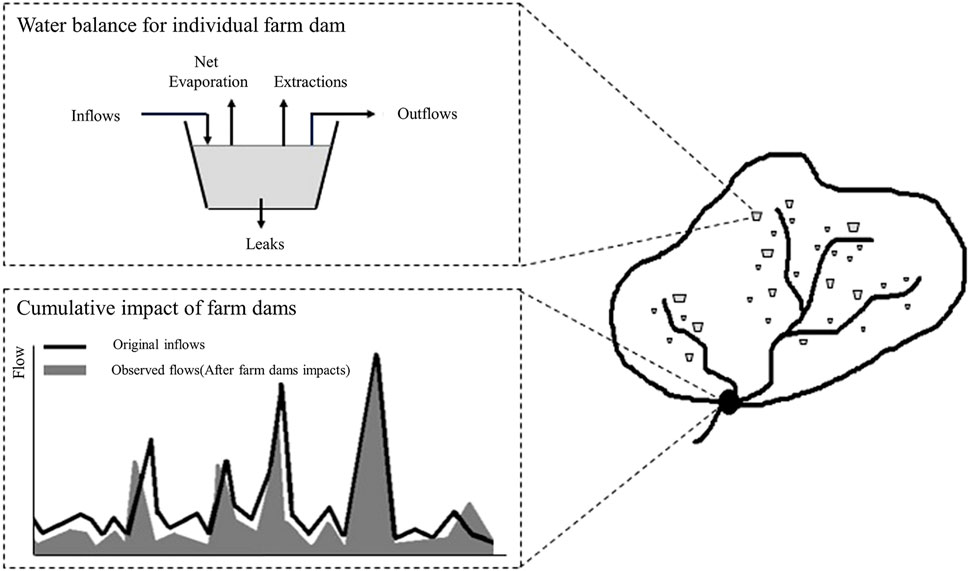
FIGURE 1. The impact of farm dams.

To better understand how hydrological processes respond to environmental changes, accurately recognizing the impact of farm dams on hydrological is essential. Hydrological models are generally used to simulate the rainfall-runoff process (Sivakumar and Berndtsson, 2010; Zainudin et al., 2012). Lumped hydrological models are widely used for the benefit of simple parameters and overall analysis of the hydrological process, although they relatively desalinate the internal differences of the basin. By measuring the storage and drainage volume of small dams, the modified flow curve could be obtained (Magilligan and Nislow, 2005). Remote sensing has been proven to be an effective tool because of its increased spatial and temporal resolution (Giri, 2012; Chen, 2018). In the past few decades, many land use product data, including Moderate Resolution Imaging Spectroradiometer (MODIS) and Advanced Very High Resolution (AVHRR), are the most widely used spatial data. However, due to the uncertainties of mixed types of land cover classification on highly dispersed areas (Zhong et al., 2016), there are some higher spatial resolution remote sensing data, e.g., Landsat TM/ETM+, and SPOT, which can clearly capture the spatial distribution of farm dams. With the development of GIS and RS, the distribution and volume of farm dams could be recognized. The distributed and semi-distributed models are widely used to reckon the effects of farm dams (Meigh, 1995; McMurray, 2006; Evrard et al., 2007; Callow and Smettem, 2009; Hughes and Mantel, 2010; Deitch et al., 2013; Ignatius and Jones, 2017). Furthermore, some researchers attached small dams to the big dam in the hydrological model to form interconnected reservoirs (Fleury et al., 2007; Fleury et al., 2009; Hughes and Mantel, 2010). However, the hydrological impacts of farm dams are different depending on their size and location, which exert varying pressures in the drainage network. If a farm dam gradually fills over time, it may no longer hinder surface runoff and even increase generation until it is drawn down again. The complexity of interactions between farm dams and river puts a damper on the combined spatial and temporal impacts of farm dams on the rainfall-runoff process (Srikanthan and Neil, 1989; Tollan, 2002).

Hydrodynamics opened a gate to better simulate the whole rainfall-runoff process at fine spatial and temporal scales in river networks (Andreadis et al., 2007; Biancamaria et al., 2009; Biancamaria et al., 2011; Durand et al., 2008; Neal et al., 2010; Neal et al., 2012). Considering inertia, pressure, gravity, friction, and momentum, it provides a detailed description of the dynamic flow movement and flood inundation areas in the drainage network. It provides a new method for simulating the hydrological process under the influence of farm dams. This model requires high-quality input data, especially topographic data (Tarekegn et al., 2010; Jarihani et al., 2015; Fernández et al., 2016). Hydrological and hydrodynamic models have their characteristics and complete each other in the details including rainfall transformation, tributary inflow. The influence of farm dams on flood wave motion could be considered by the hydrological–hydrodynamic coupled models. Advanced remote sensing technology can provide high-resolution data for the dynamic movement of water flow.

In order to make reasonable decisions in water resources management, an integrated understanding of how impacts of farm dams vary in time and space on the rainfall-runoff process is needed. The natural effects of farm dams, which influence peak discharge and peak appearance time of floods, are the direct effect of the network on the flood routing. Therefore, the motivation for this study is to apply a suitable tool to reckon the impact of farm dams on the rainfall-runoff process. The Xinlicheng Reservoir Basin with numerous farm dams is taken as the study area. The feasibility and effect of the coupled model were verified based on the probability of occurrence at a given time or exceeding a certain threshold against typical floods. The paper is structured as follows: The Methodology section presents the methodology, the Study area and data processing section depicts the study area and dataset, the Results section casts light on discussions, and the Discussion section gives out the conclusion.

2 Methodology

Ideally, a rainfall-runoff model is trying its best to fit the observed data, with parameters being calibrated jointly with the impact of farm dams. Except for magnitude, the timing, frequency, and distribution of flow are critical to simulate accurately.

2.1 Hydrological Model

Considering as a mature conceptual model, the three-source XAJ model is widely used in humid and semi-humid areas, which is good at simulating the rainfall-runoff process for a basin at a large scale (Zhao, 1992; Jayawardena and Zhou, 2000; Cheng et al., 2002; Li et al., 2009; Ju et al., 2009). The model has a total of 16 parameters and the input of the model is rainfall and evaporation. The soil structure is divided into three layers: loose layer, compact layer, and groundwater aquifer. The underlying surface of the basin is divided into permeable areas and impermeable areas. The runoff composed of surface runoff, interflow, and underground runoff in underlying surface is developed by the runoff yield under excess infiltration theory. The runoff is developed by the runoff yield under excess infiltration theory, and the runoff is composed of surface runoff, interflow, and underground runoff. The surface runoff is calculated by the unit hydrograph. The interflow and groundwater flow are routed by the linear reservoir method. The flowchart is presented in Figure 2. For more information about the XAJ model and the detailed equations used in the model, please refer to Zhao (1992).

FIGURE 2

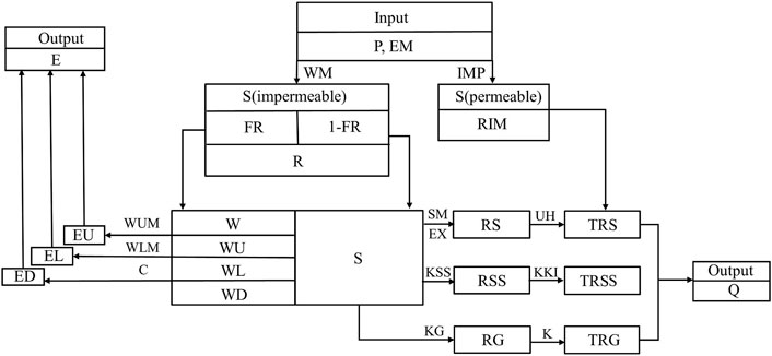
FIGURE 2. Flow chart for the Xinanjiang model (XAJ) model (Zhao, 1992). Note: P, precipitation; EM, potential evaporation; S, free water storage; FR, area ratio with runoff generation; W, total soil moisture; WU, upper layer soil moisture; WL, lower layer soil moisture; WD, deeper layer soil moisture; EU, upper layer soil evaporation; EL, lower layer soil evaporation; ED, deeper layer soil evaporation; E, actual evaporation; WUM, the soil water storage capacity of upper layer; WLM, the soil water storage capacity of lower layer;, C, coefficient of deep evapotranspiration; SM, areal mean of the free water capacity of the surface soil layer; EX, exponent of the free water capacity curve; KSS, outflow coefficients of the free water storage to interflow; KG, outflow coefficients of the free water storage to groundwater; KKI, recession constant of the lower interflow storage; K, recession constant of groundwater storage; UH, unit hydrograph; KG, coefficient of groundwater runoff; R, runoff generation; RS, surface runoff; RSS, interflow runoff; RG, groundwater runoff; TRS, surface discharge; TRSS, interflow discharge; TRG, groundwater discharge; Q, basin discharge.

2.2 Hydrodynamic Model

The conservation form of the governing equation of the two-dimensional shallow water equations are as follows:

$\frac{\mathbf{\partial }\mathbf{q}}{\mathbf{\partial }\mathbf{t}}+\frac{\mathbf{\partial }\mathbf{f}}{\mathbf{\partial }\mathbf{x}}+\frac{\mathbf{\partial }\mathbf{g}}{\mathbf{\partial }\mathbf{y}}=\mathbf{s}(1)$

where $\text{q}$ is the vector of conserved flow variables, f and g are the flux vectors in the x and y Cartesian directions, $t$ is the time, and $\text{s }$ is the source terms.

$\text{q}=\left[\begin{array}{c}\mathit{h}\\ \mathit{hu}\\ \mathit{hv}\end{array}\right],\text{f}=\left[\begin{array}{c}\mathit{hu}\\ {\mathit{u}}^2\mathit{h}+\frac{1}{2}\\ \mathit{uvh}\end{array}\mathit{g}{\mathit{h}}^2\right],\text{g}=\left[\begin{array}{c}\mathit{hv}\\ \mathit{hvu}\\ \mathit{h}{\mathit{v}}^2+\frac{1}{2}\mathit{g}{\mathit{h}}^2\end{array}\right](2)$

$\text{S}=S_0+S_f+R=\left[\begin{array}{c}\begin{array}{c}\mathit{r}\\ -\frac{{\mathit{\tau }}_{\mathit{mx}}}{\mathit{\rho }}-\mathit{gh}{\mathit{S}}_{\mathit{fx}}\end{array}\\ -\frac{{\mathit{\tau }}_{\mathit{my}}}{\mathit{\rho }}-\mathit{gh}{\mathit{S}}_{\mathit{fy}}\end{array}\right](3)$

${\mathit{S}}_{\mathit{fx}}=-\frac{\partial {\mathit{n}}_{\mathit{m}}}{{\partial }_{\mathit{x}}},{\mathit{S}}_{\mathit{fy}}=-\frac{\partial {\mathit{n}}_{\mathit{m}}}{{\partial }_{\mathit{y}}}(4)$

${\mathit{\tau }}_{\mathit{mx}}=\rho C_{\mathbf{f}}u\sqrt{u^2+v^2},{\mathit{\tau }}_{\mathit{my}}=\rho C_{\mathbf{f}}v\sqrt{u^2+v^2}(5)$

where $g$ is the gravitational acceleration; $h$ is the water depth ($h=\eta -Z_b$ , where $\eta$ is the water surface elevation and $Z_b$ is the bed elevation); $\rho$ is the water density; $u$ and $v$ are the depth-averaged flow velocities in the $x$ and $y$ Cartesian directions; $n_m$ is the river bottom elevation; $S_0$, $S_f$, and $R$ are the source terms of bed slope, friction, and rainfall; $S_{fx}$ and $S_{fy}$ are the bottom friction in the $x$ and $y$ Cartesian directions; ${\mathit{\tau }}_{\mathit{mx}}$ and ${\mathit{\tau }}_{\mathit{my}}$ are the bed friction stresses; $C_f$ is the bed roughness coefficient ($C_f=g{n}^2/h^{\frac{1}{3}}$); and n is the Manning’s coefficient.

For the implementation of the numerical scheme, the calculation results of velocity, direction, and water depth from the upstream grid are transmitted to the downstream adjacent grid by using a finite volume shock-capturing Godunov-type scheme incorporated with the HLLC approximate Riemann solver. At the same time, aiming at the problem that is difficult to get the calculation results quickly, the parallel algorithm is designed based on the high-performance computing technology of GPU in the CUDA development platform. So far, a coupled hydrological and hydrodynamic model can be established, which can seamlessly integrate the water from the upstream in the horizontal direction and the surface runoff falling vertically to simulate the surface process of a flood, compared with the observed runoff data to verify the effect of the coupled model.

2.3 Coupled -XAJ Model

Owing to the existence of multiply farm dams and other spatial projects, the original continuous process of surface runoff calculated by unit hydrography may appear large mutation or no response. Remote sensing could provide continuous observation with high temporal and spatial resolution in the whole basin. The coupled XAJ model adapts hydrodynamics with remote sensing data to replace the confluence part. The storage capacity curve is the core of the XAJ model. By using the XAJ model, the tension water storage capacity curve and the free water storage capacity curve can be obtained. In terms of the runoff yield of different land types, the above curves are discretized to obtain the surface runoff on different grids. The amount of water from the upstream, the vertical surface runoff from the hydrological model, and different remote sensing datasets including DEM, land use, and Manning coefficient are input into the hydrodynamic model.

By the conservation of mass and momentum, the calculation results of velocity, direction, and water depth from the upstream grid are transmitted to the downstream adjacent grid, so as to obtain the dynamic process. The relationship between incoming and outgoing water in the farm dams of the whole basin is mainly dependent on its drainage area and the actual water surface so that the hydro-hydrodynamic model can solve the problem brought by farm dams. The output surface runoff of the hydrodynamic model, with the interflow and groundwater flow of the XAJ model, constructed the total runoff (Figure 3), which is compared with the observed runoff data to verify the effect of the coupled model.

FIGURE 3

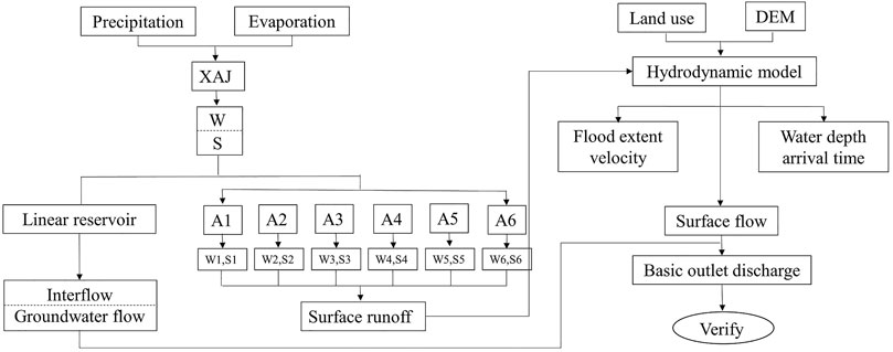
FIGURE 3. Flow chart of the coupled XAJ. Note: W, tension water storage capacity curve; S, free water storage capacity curve; W1, tension water storage capacity curve of farmland; W1, tension water storage capacity curve of farmland; W2, tension water storage capacity curve of forest land; W3, tension water storage capacity curve of grassland; W4, tension water storage capacity curve of water body; W5, tension water storage capacity curve of urban area; W6, tension water storage capacity curve of unused land; S1, free water storage capacity curve of farmland; S2, free water storage capacity curve of forest land; S3, free water storage capacity curve of grassland; S4, free water storage capacity curve of water body; S5, free water storage capacity curve of urban area; S6, free water storage capacity curve of unused land; A1, the area of farmland; A2, the area of forest land; A3, the area of grassland; A4, the area of water body; A5, the area of urban area; A6, the area of unused land.

3 Study Area and Data Processing

3.1 Study Area and Human Activities

The Xinlicheng Reservoir Basin (XLCRB) is located in the southeast of Changchun City, Jilin Province (43° 3′–43° 44′N, 125° 0'–125° 37′E) (Figure 4). Its economy is dominated by agriculture, including rainfed and some irrigated agriculture. The demand for water use, needed for irrigation, human and animal use, is mainly from precipitation. Lying in the semi-arid and semi-humid monsoon climate area, it has a high variable rainfall distribution in time and space. The rainy season is from June to October, accounting for more than 75% of the annual rainfall in total. In order to make full use of water resources during the rainy season and prevent water scarcity in the dry season, Xinlicheng Reservoir is constructed by intercepting Yitong River from Yinma River tributary of Songhua River, ensuring the production and domestic water use for Changchun City.

FIGURE 4

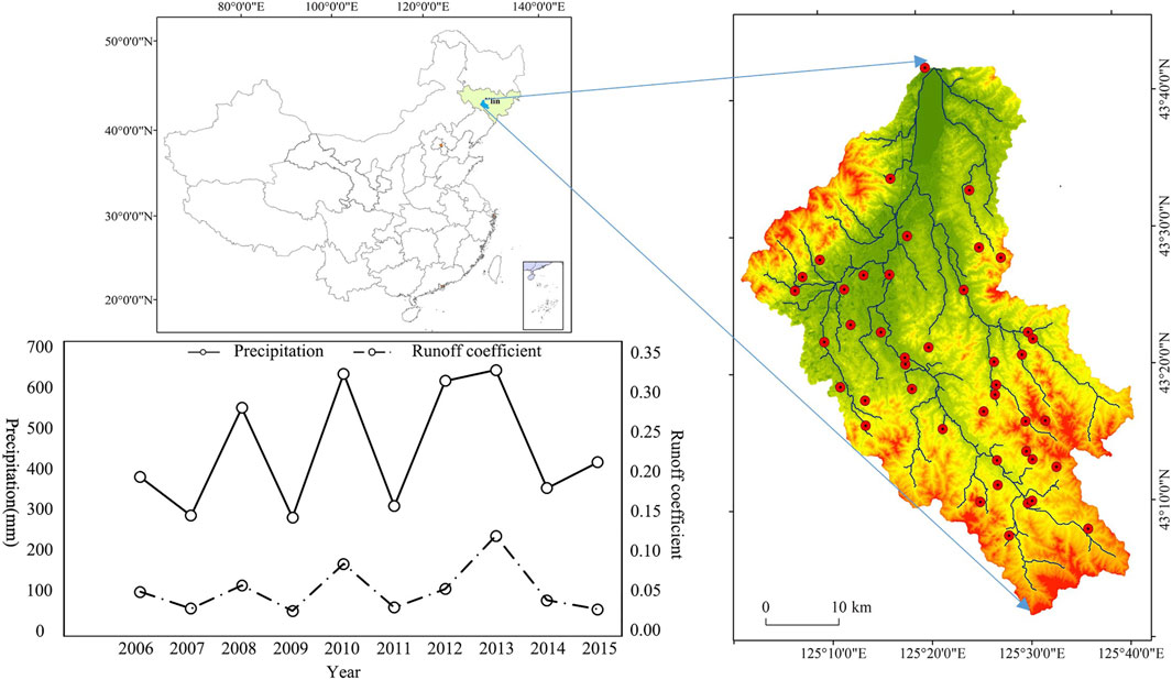
FIGURE 4. Location of the Xinlicheng Reservoir Basin (XLCRB).

In the past few decades, the runoff in XLCRB has a statistically significant downward trend (except 2013). This may be due to urbanization, increasing agricultural activity, and drought events. Farmland is the major land use form, accounting for around 60% of the area. It was found by field investigation, that farmers built lots of private farm dams in proximity to places of demand beyond government regulation, which gathered surface runoff during the rainy season to ensure water consumption. They are scattered throughout the basin. Among them, the smallest ones are full at the end of the rainy season and dry out before the end of the dry season. Although they are important for water use guarantee, it resulted in a complex and dense farm dams network for their open morphology, which was extremely difficult to manage. Therefore, it is critical to know the antecedent conditions of runoff, particularly in basins with multiple smaller on-farm dams. It will be beneficial to have efficient, small, and medium-scale flood resources management, to alleviate the conflict problem of rural water use.

3.2 Dataset

To simulate the hydrological process in the XLCRB, we need data as described below:

1) Regional map, with river network and reservoirs.

2) Hydrological data: Precipitation, potential evapotranspiration, and runoff (2006–2015) from the local administration. The data were first interpolated to grids using an angular distance weighting method since the local administration are sparse and unevenly distributed in the study area.

3) Remote sensing data: digital elevation model (DEM), land use type, and so forth.

4) In addition, Manning coefficient representing surface roughness is needed.

The DEM data were obtained from the SRTM 30 m × 30 m Digital Elevation Data.

The land use types were extracted with Landsat 8 OLI_TIRS, which was provided by the Geospatial Data Cloud site (http://www.gscloud.cn). We chose the images from 2006 to 2015 and classified the land use type by supervised method for simulation. In order to reflect the local land use change more clearly, the land use image of 2006, 2008, 2012, and 2015 were chosen to display. We chose the images of the years 2006, 2008, 2012, and 2015, and classified the land use type by the supervised method. The land use categories of XLCRB were classified into six kinds based on ground survey and land cover maps, including farmland, forest land, grassland, water, urban land, and unused land.

Surface roughness is an important index to reflect the surface condition that delays the surface runoff, which is affected by many factors such as section geometry, land-cover type, the material composition of the riverbed, terrain change, time, and so on. Surface roughness is mainly based on the land use type. Different land use types have different roughness values. The Manning coefficient adopted by the experiment of Chen (2017) is used to reflect the surface roughness in this paper (Table 1).

5) Reservoir information. There is only one large reservoir in the study area, the Xinlicheng Reservoir. The reservoir information included the reservoir name, year of completion, controlled basin area, reservoir capacity, and reservoir function.

TABLE 1

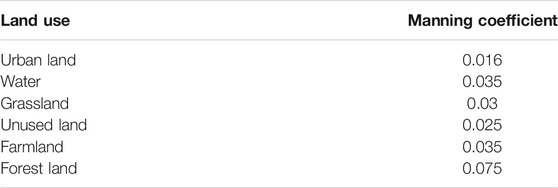
TABLE 1. Manning coefficient.

3.3 Evaluation Criteria

Several objective indicators were used to measure the results of the model: The Nash–Sutcliffe Efficiency Coefficient (NS) (Nash and Sutcliffe, 1970), Relative Error of Flood Discharge (REFD), and Difference of Peak Appearance Time (DPAT) are used to evaluate the model. When the value of REFD is between (−0.2, 0.2), it is qualified; when the value of $\text{NS}$ is over 0.5, it is considered good, and in the interval (0.36, 0.75), it can be acceptable (Motovilov and Kolganova, 1999).

The comparison criterion of Nash is defined by the following formula

$\text{NS}=1-\frac{{\displaystyle \sum {\left(Q_o-Q_c\right)}^2}}{{\displaystyle \sum {\left(Q_o-Q_o\right)}^2}}(6)$

$\text{REFD}=\frac{{\displaystyle \sum Q_c}-{\displaystyle \sum Q_o}}{{\displaystyle \sum Q_o}}(7)$

where $Q_o$ is the observed discharge (m³/s), $Q_c$ is the calculated discharge (m³/s), and $Q_o$ is the mean of observed discharge (m³/s);

$\text{DPAT}=T_{Q_{c\text{(max)}}}-T_{Q_{o\text{(max)}}}(8)$

where $T_{Q_{c\text{(max)}}}$ is the calculated flood peak appearance time, and $T_{Q_{o\text{(max)}}}$ is the observed flood peak appearance time.

3.4 Model Setup in the XLCRB

3.4.1 Hydrological Model

There are relatively complete meteorological data for 10 years (from 2006 to 2015) of the basin, and they were used for simulation. The average precipitation of the study area was 432 mm/year during the period. The XAJ model input parameters were derived via actual observed rainfall and streamflow data. The data for the first 2 years were used for preheating, the next 3 years for calibrating, and the rest of the years for verification. The results of the parameter calibration are presented in Table 2.

TABLE 2

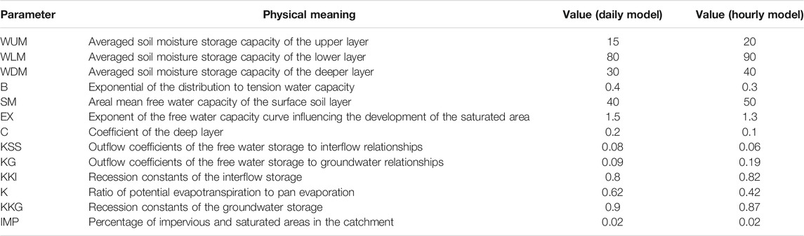
TABLE 2. The parameters of XAJ model.

Based on the existing rainfall, evaporation, and runoff data of the basin, the water storage capacity curve of the basin was obtained through parameter calibration. The water storage capacity curve was discretized for various characteristics of land-use runoff generation. The water storage capacity value on each grid was calculated to obtain the runoff yield and surface runoff of each grid in each period.

The parameters of hydrological process have spatial heterogeneity. Different underlying surface conditions (vegetation cover, land use, topography, and soil) have various parameters that are different. In order to obtain accurate model parameters, a large number of observation points must be arranged for further observation. However, the existing measurement methods at a watershed scale are not realistic.

3.4.2 Hydrodynamic Model

Hydrodynamic model is an event-based model, which is not continuous. In order to avoid the interference of artificial setting soil moisture and groundwater runoff on the calibration results, the data of daily model are used to set the soil moisture and groundwater runoff of the hourly model. During model setup, meteorological, topographic, land use, and soil data are integrated to run the hydrodynamic model. A total of 4,765,772 cells of 30 m × 30 m resolution are used to solve the shallow water equations to simulate the flooding process.

4 Results

4.1 Land Use Change

The increase or decrease in land use type is the most intuitive reflection of land use change. By analyzing various types of area change, we can understand the overall trend of regional land use. According to the interpretation results, the area of different land use types in XLCRB is counted, and the results are shown in Table 3 and Figure 5. It can be seen that farmland and forest land are the main land use types, accounting for more than 89% of the basin area. Among them, farmland is the main land use type, accounting for 59.46%, followed by forest land, which is concentrated in the southeast, with high vegetation coverage. The area of water and urban land showed a more or less similar proportion, and the area of unused land is the smallest.

TABLE 3

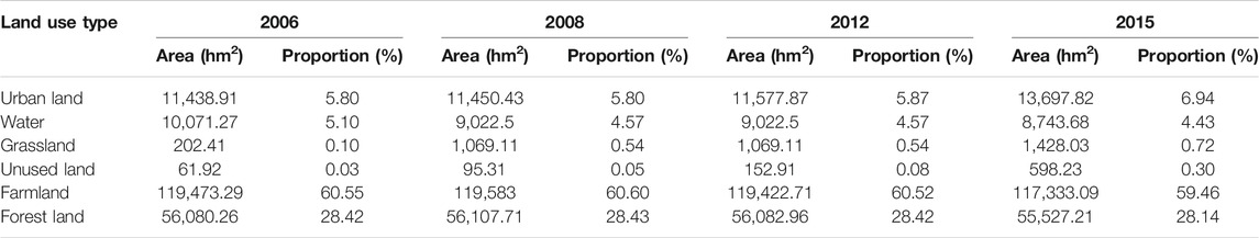
TABLE 3. Area statistics of different land types in different periods.

FIGURE 5

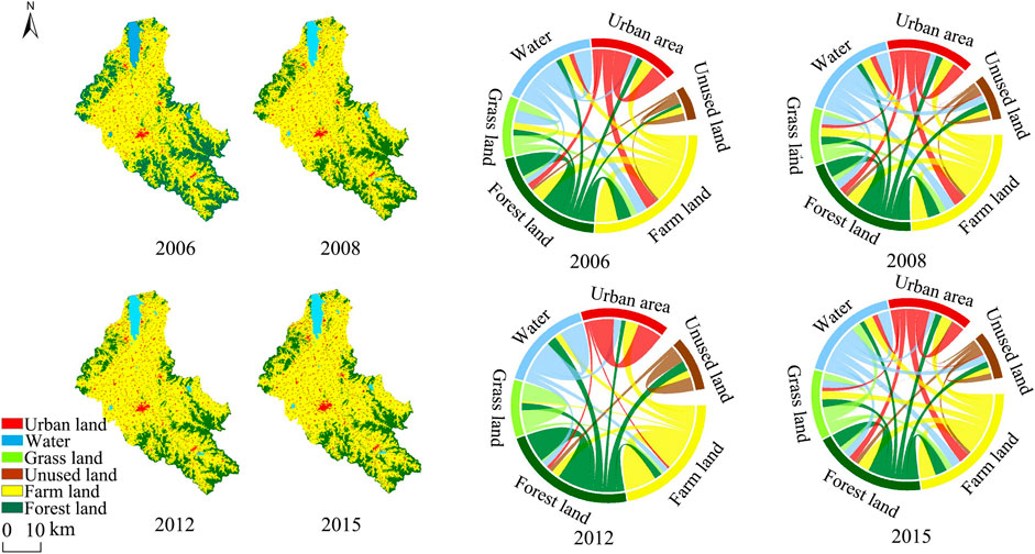
FIGURE 5. The distribution and conversion of land use in 2006, 2008, 2012, and 2015.

During these 9 years, the area of farmland decreased from 119,473.29 to 117,333.09 km². Although the total values changed a little, the inflow and outflow changed greatly. The urban land in the basin generally showed an increasing trend, and it increased significantly faster than other land types, which showed high consistency. The increased construction land was mainly transformed from farmland. At the same time, in order to ensure the “eight hundred million hectares of the arable land red line” and make up for the loss of farmland, the government reclaimed farmland in mountainous areas or unused land to achieve the cultivated land balance.

4.2 Modeling Results

4.2.1 Daily Results

By comparing the simulated and observed discharge at the catchment outlet from 2006 to 2015, the results are evaluated by charts (Figure 6) and statistics (Table 4). By satisfactory performance in visual and statistical comparisons, the calibration process was passed. During the validation, the model was processed with a defined value of calibration parameters. The fitting effect is not good on account of the incompleteness of the data in some years. The value of REFD in other years is controlled within 20%, and the value of NS is more than 0.5. It can be seen that the observed flow hydrograph is in agreement with the simulated flow hydrograph. The mean value of the NS coefficient from 2006 to 2015 is about 0.6, and the mean value of relative error is about 0.123.

FIGURE 6

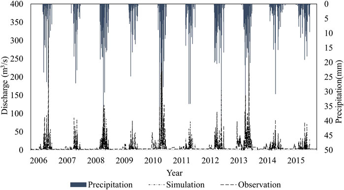
FIGURE 6. The results of the daily model for the XAJ model from 2006 to 2015.

TABLE 4

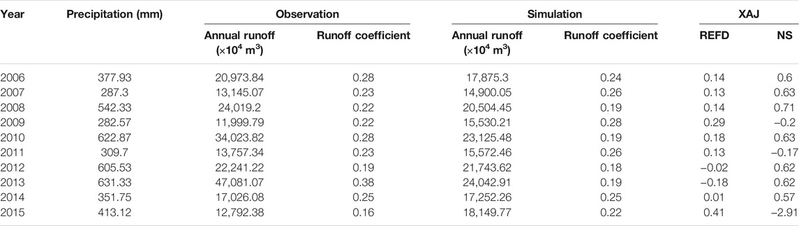
TABLE 4. The simulation of daily model for the XAJ model.

4.2.2 Hourly Results

The results of the XAJ model are presented to better verify the effect of the coupled XAJ (Table 5) (Figure 7).

TABLE 5

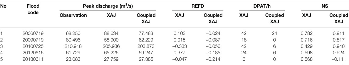
TABLE 5. The simulation of hourly model for the XAJ model and the coupled model.

FIGURE 7

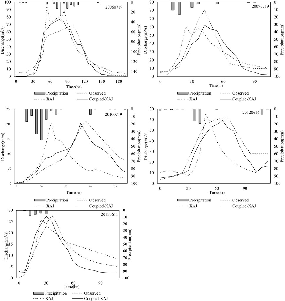
FIGURE 7. Results of the flood hydrograph.

Based on the results, for peak discharge, most peak discharges simulated by the XAJ model is larger than the observed since the retaining effect of the farm dams is not considered. Meanwhile, the peak appearance time is delayed. Among them, the simulated peak discharge of No. 20090719 is much smaller. The probable reason is that farm dams are filled with the previous flood leading to expansion of runoff area.

The developed Coupled-XAJ model shows great performance in these five typical flood events. For peak discharge and DPAT, the coupled XAJ model plays better, which is also the fundamental purpose of adding the hydrodynamic model. Hydrodynamics capture the underlying characteristics of the basins and solve the problem of nonlinearity in the confluence process. The value of NS efficiency indicates that the model could reproduce 81%–92% of the variability observed in the hydrographs as all observed flows are closely matched by the model predictions. The flood hydrographs closed to the actual situation verify that the coupled XAJ model plays an active role in simulating the effect of farm dams on flood peak.

The large number and uneven distribution of farm dams play an important role in the timing, magnitude, and frequency of flow, and affect the spatial range of flow variation. With the application of hydrodynamic model, the water depth and flow velocity in each grid and each time point of flood routing can be obtained to help comprehend the spatial distribution of flood variation under the influence of farm dams. Large floods may destroy insecure farm dams and cause cumulative effects. The special information including the maximum submergence depth, the maximum velocity, and the arrival time of the maximum submergence depth make us better estimate the flood risk and provide reliable technical support for flood forecasting.

5 Discussion

5.1 Farm Dam

Farm dam is an appropriate tool to utilize small-scale and relatively frequent floods for drought and flood mitigation. Although it reaches a wide population and facilitates its water demands, in turn, it has effects on the hydrological process.

To answer questions from a hydrologic point of view and have effective water resource management, it is necessary to quantify the spatial distribution of farm dams. The large uncertainty in farm dam development time and size on account of privacy nature is a constraint (Dare et al., 2002; Shao et al., 2012). In order to obtain information about the location and quantity of farm dams, many surveys were carried out. Many scholars used the surface area to monitor the storage capacity of small farm dams by empirical formula (Nathan et al., 2005b). With the development of GIS and RS, the National River Health Programme (2002) adapted the topographic map, and later, some scholars used the digital topographic information to count the number and extent of small farm dams (Nathan et al., 2005a; Lett et al., 2009; Martinez et al., 2010).

The Xinlicheng reservoir and the generous farm dams form open water, accounting for 4.4% of the land surface. Farm dams and water bodies were extracted from high-resolution digital elevation models. A typical rainy season when the farm dams were expected to be full is chosen, so the maximum surface areas of the farm dams could be captured. It is difficult to explain the full capacity when most farm dams were half full or less full. Maximum likelihood classification (Mather, 1999) was used to extract farm dams, and the 3D analyst module of ArcGIS is used to calculate the volume of the farm dams. The commonly used method called trigonometric grid is adopted to divide the water body into triangular prisms in terms of the actual shape of the waterbody. The volume of the whole pond is obtained by summing the volume of each prism. The mathematical model is as follows:

$\text{V}={\displaystyle \sum }_{i=1}^n{P}_i\left(H-\frac{h_i+h_{i+1}+h_{i+2}}{3}\right)(9)$

where V is the volume of the pond, $P_i$ is the area of a single triangular, H is the elevation of the specified water level, $h_i$ is the elevation of the triangular grid, and $n$ is the number of triangular grids.

The classification obtained a total of 72 farm dams with a total volume of more than 6 × 108 m³. Given the 30-m resolution of the Landsat imagery, some farm dams were deleted from the dataset because the likelihood of incorrectly identifying very small features is high. Some certain reservoirs controlled by the government were also discarded. The spatial distribution of farm dams is shown in Figure 8. Though the spatial distribution of farm dams is related to valley shape, topographic premises, and other factors, most farm dams are located in proximity to places of demand with agricultural land uses. The huge amount and uneven distribution further prove that farm dams play an important role in this area. The mapping of farm dams would help to better understand the water balance and simulate the rainfall-runoff process, thus, providing reasonable advice for effective water management planning.

FIGURE 8

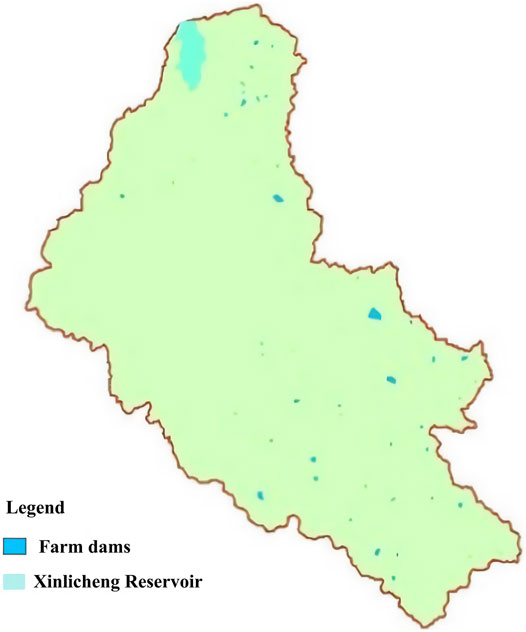
FIGURE 8. The distribution of farm dams in XLCRB.

5.2 Feasibility of Integrated Simulation

As a largely agricultural country, the small-scale farm dams in rural areas in China are widely developed. Most of them are Earth dams with a clay core. Due to the private nature and the inequity of water storage, droughts and floods may be more serious. Insecurity farm dams, especially privately-owned farm dams, may lead to cumulative failure during large floods (Lewis and Harrison, 2002; Bocchiola and Rosso, 2014), and overtopping is the major form of dam failure (Foster et al., 2011). Even small floods would cause cumulative results (Pisaniello, 2009), which is not usually considered in the typical flood study with regard to related flood damage. In China, the Shimantan and Banquia dams failed in 1975 due to the cumulative failure of 60 small upstream dams, resulting in 230,000 deaths (Si and Quing, 1998). It affects the dynamic balance of the water cycle and increases the frequency and intensity of floods. Thus, it can be seen that flood events caused by farm dams are also worthy of attention.

In recent years, with the rise of remote sensing technology, more detailed topographic data and river section data make the hydrodynamic model more applied in analyzing and evaluating flood risk. The necessary input of flow data is provided by the hydrological model. Therefore, the coupled hydro-hydrodynamic model has been gradually applied to basins with different scales at home and abroad (Table 6). The development and application of the coupled models also prove a possibility of practical application. There are different ways to realize the coupling of hydrology and hydrodynamics, including external coupling or loose coupling, internal coupling, and full coupling.

TABLE 6

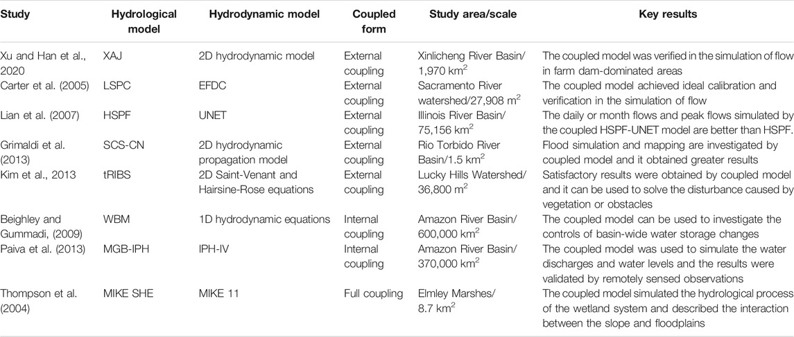
TABLE 6. Research on the coupled hydro-hydrodynamic model.

The coupled XAJ uses external coupling mode, which takes the output of one model as the input of another model, which is usually regarded as the simplest and most effective coupling mode. It does not need to modify the model code and maintain the independence and integrity of the model components, meaning that hydrodynamic effects would not affect the hydrological model. The XAJ model is proven to simulate the whole rainfall-runoff process, and the hydrodynamic model has high-speed calculation. Thus, the coupled model provides a new method to weigh the complex influence of farm dams on the hydrological process of the basin and utilize water resources in farm dam-dominated areas better.

The hydro-hydrodynamic model can be used in many other aspects. The data used in the coupled model can be obtained through measurement or remote sensing data. If the basin does not have a large number of measured flows for calibration, it can still be modeled through these physically meaningful data to calculate the runoff yield, so as to simulate the confluence process. Therefore, the approach is also applicable to other ungauged basins; this is what we will further study and verify. The quantitative relationship between land-use change factors and surface runoff can be established to provide quantitative spatial and temporal analysis for the disturbance of land-use activities on the hydrological process. It can provide technical support and a theoretical basis for the comprehensive formulation of land-use planning and flood control planning.

5.3 Limitations

The uncertainty arises from many aspects. The losses of farm dams (draft, seepage, and evaporation) are normally considered to be small, which are neglected. Other factors may influence flow variation, such as urban expansion and climate change. More importantly, due to the high degree of complexity in the interaction between farm dams and runoff, the scale of the simulated flood is relatively small, which could not tell the whole story. For larger events, it is easy to exceed the capacity of the dam, and the final impact of the dam on large-scale flood discharge may be relatively small. However, in most rainfall events of a year, they obviously have a significant impact on flow prediction. With the aggregation of farm dams in a basin, how this affects relationships between runoff, storage, spillage, and evaporation losses, and how this change in land use, surface hydrology, and atmospheric feedback, all need to be evaluated more closely. From Figure 7, we can see that the accuracy of the confluence part needs to be improved. After analysis, most of these rainfall processes occur in June and July, which is the growing season of crops. From Figure 6 and Table 4, we can also see that there is a certain simulation error in the confluence. It may be that artificial water storage is used for crop growth, resulting in interference in the confluence process and some errors.

6 Conclusion

With the increasing demand for water resources, spatially distributed projects like farm dams have been constructed around the world. The large number and uneven distribution of farm dams have a non-ignorable impact on the timing, magnitude, and frequency of flow variation. Under the impacts of growing anthropogenic activities and substantial environmental changes, how to manage water resources in a sustainable way is a crucial problem. However, accurate estimation of the rainfall-runoff process is still facing great challenges as a result of the unknown information about farm dams. In this study, hydro-hydrodynamics provides a method for this situation. In the portion of XLCRB, five real precipitation events were used to evaluate, which cast light on the coupled XAJ, which considered that the impacts of farm dams provided the improvement in the accuracy of peak discharge and peak appearance time compared with the XAJ model, which showed that the model can provide important technical support for flood control prediction and disaster assessment of the basin.

The hydro-hydrodynamics model not only explains “whether there is an overall impact” and “how is the overall impact” on the whole process but also states “where has an impact” and “how the degree of impact.” Its development is of great significance for quantifying the changes in hydrological processes under the influence of human activities, and it could enable future scenarios to be simulated from input data. The approach has been designed to be applicable to any catchment, whether gauged or ungauged.

Data Availability Statement

The original contributions presented in the study are included in the article/supplementary material, further inquiries can be directed to the corresponding author.

Author Contributions

CX, ZH, and HF contributed to the conception and design of the study. CX organized the hydrological database and ran the model. ZH performed the statistical analysis land use process. HF was responsible for the project administration. ZH wrote the first draft of the manuscript. CX, ZH, and HF wrote sections of the manuscript. All authors contributed to the manuscript revision, and read and approved the submitted version.

Funding

This research was funded by the Major Science and Technology Program for Water Pollution Control and Treatment, grant number No. 2014ZX07203-008.

Conflict of Interest

The authors declare that the research was conducted in the absence of any commercial or financial relationships that could be construed as a potential conflict of interest.

Publisher’s Note

All claims expressed in this article are solely those of the authors and do not necessarily represent those of their affiliated organizations, or those of the publisher, the editors, and the reviewers. Any product that may be evaluated in this article, or claim that may be made by its manufacturer, is not guaranteed nor endorsed by the publisher.

References

Andreadis, K. M., Clark, E. A., Lettenmaier, D. P., and Alsdorf, D. E. (2007). Prospects for River Discharge and Depth Estimation through Assimilation of Swath‐altimetry into a Raster‐based Hydrodynamics Model. Geophys. Res. Lett. 34 (10), 265–578. doi:10.1029/2007gl029721

CrossRef Full Text | Google Scholar

Ashraf, M., Kahlown, M. A., and Ashfaq, A. (2007). Impact of Small Dams on Agriculture and Groundwater Development: A Case Study from Pakistan. Agric. Water Manag. 92 (1-2), 90–98. doi:10.1016/j.agwat.2007.05.007

CrossRef Full Text | Google Scholar

Beighley, R. E., and Gummadi, V. (2011). Developing Channel and Floodplain Dimensions with Limited Data: a Case Study in the Amazon Basin. Earth Surf. Process. Landforms 36 (8), 1059–1071. doi:10.1002/esp.2132

CrossRef Full Text | Google Scholar

Biancamaria, S., Bates, P. D., Boone, A., and Mognard, N. M. (2009). Large-scale Coupled Hydrologic and Hydraulic Modelling of the Ob River in Siberia. J. Hydrol. 379 (1-2), 136–150. doi:10.1016/j.jhydrol.2009.09.054

CrossRef Full Text | Google Scholar

Biancamaria, S., and Durand, M. (2011). Assimilation of virtual wide swath altimetry to improve Arctic river modeling. Remote Sensing of Environment 115 (2), 371–381.

CrossRef Full Text | Google Scholar

Bocchiola, D., and Rosso, R. (2014). Safety of Italian Dams in the Face of Flood hazard. Adv. Water Resour. 71, 23–31. doi:10.1016/j.advwatres.2014.05.006

CrossRef Full Text | Google Scholar

Braccia, M., and Hall, J. (2014). “Localised Rainfall Runoff Modelling to Estimate Farm Dam Inflows and Reliabilities,” in Hydrology and Water Resources Symposium (Barton, ACT: Engineers Australia), 921–928.

Google Scholar

Callow, J. N., and Smettem, K. R. J. (2009). The Effect of Farm Dams and Constructed banks on Hydrologic Connectivity and Runoff Estimation in Agricultural Landscapes. Environ. Model. Softw. 24 (8), 959–968. doi:10.1016/j.envsoft.2009.02.003

CrossRef Full Text | Google Scholar

Carter, S., Denton, D., Sievers, M., Von Loewe, P., and Craig, J. (2005). Hydrologic Model Development of the Sacramento River Watershed to Support TMDL Development. Proc. Water Environ. Fed. 2005 (3), 1542–1570. doi:10.2175/193864705783966909

CrossRef Full Text | Google Scholar

Cescato, I. (2018). Modelling the Water Balance and Hydrologic Dynamics of a Farm Dam. Adelaide, Australia: Doctoral dissertation, Flinders University, College of Science and Engineering.

Google Scholar

Cetin, L. T., Mosley, L. M., Jordan, P. W., Authority, E. P., and Mertz, S. K. (2009). “January)Assessing the Impacts of Farm Dams on the Streamflow of the Mount Lofty Ranges Watershed,” in Proc. Hydrology and Water Resources Symposium (Newcastle.

Google Scholar

Chen, X., Jiang, J., and Li, H. (2018). Drought and flood monitoring of the Liao River Basin in Northeast China using extended GRACE data. Remote Sensing 10 (8), 1168.

CrossRef Full Text | Google Scholar

Cheng, C., Ou, C., and Chau, K. W. (2002). Combining a Fuzzy Optimal Model with a Genetic Algorithm to Solve Multi-Objective Rainfall-Runoff Model Calibration. J. Hydrol. 268 (1-4), 72–86. doi:10.1016/s0022-1694(02)00122-1

CrossRef Full Text | Google Scholar

Dare, P., Fraser, C., and Duthie, T. (2002). Application of Automated Remote Sensing Techniques to Dam Counting. Australas. J. Water Resour. 5 (2), 195–208. doi:10.1080/13241583.2002.11465204

CrossRef Full Text | Google Scholar

de Araújo, J. C., and Medeiros, P. H. A. (2013). Impact of Dense Reservoir Networks on Water Resources in Semiarid Environments. Australas. J. Water Resour. 17 (1), 87–100. doi:10.7158/13241583.2013.11465422

CrossRef Full Text | Google Scholar

Deitch, M. J., Merenlender, A. M., and Feirer, S. (2013). Cumulative Effects of Small Reservoirs on Streamflow in Northern Coastal California Catchments. Water Resour. Manag. 27 (15), 5101–5118. doi:10.1007/s11269-013-0455-4

CrossRef Full Text | Google Scholar

DSE (2007), Your Dam Your Responsibility, A Guide to Managing the Safety of Farm Dams. Irrigation and Commercial Farm Dams, License to Water. Victoria: Department of Sustainability and Environment, 90.

Google Scholar

Durand, M., Andreadis, K. M., Alsdorf, D. E., Lettenmaier, D. P., Moller, D., and Wilson, M. (2008). Estimation of Bathymetric Depth and Slope from Data Assimilation of Swath Altimetry into a Hydrodynamic Model. Geophys. Res. Lett. 35 (20). doi:10.1029/2008gl034150

CrossRef Full Text | Google Scholar

Evrard, O., Persoons, E., Vandaele, K., and Van Wesemael, B. (2007). Effectiveness of Erosion Mitigation Measures to Prevent Muddy Floods: a Case Study in the Belgian Loam belt. Agric. Ecosyst. Environ. 118 (1-4), 149–158. doi:10.1016/j.agee.2006.02.019

CrossRef Full Text | Google Scholar

Fernández, A., Najafi, M. R., Durand, M., Mark, B. G., Moritz, M., Jung, H. C., et al. (2016). Testing the Skill of Numerical Hydraulic Modeling to Simulate Spatiotemporal Flooding Patterns in the Logone Floodplain, Cameroon. J. Hydrol. 539, 265–280. doi:10.1016/j.jhydrol.2016.05.026

CrossRef Full Text | Google Scholar

Fleury, P., Ladouche, B., Conroux, Y., Jourde, H., and Dörfliger, N. (2009). Modelling the Hydrologic Functions of a Karst Aquifer under Active Water Management–The Lez spring. J. Hydrol. 365 (3-4), 235–243. doi:10.1016/j.jhydrol.2008.11.037

CrossRef Full Text | Google Scholar

Fleury, P., Plagnes, V., and Bakalowicz, M. (2007). Modelling of the functioning of karst aquifers with a reservoir model: application to Fontaine de Vaucluse (South of France). Journal of Hydrology 345 , 38–49.

CrossRef Full Text | Google Scholar

Foster, I. D. L., Collins, A.L., and Naden, p. S. (2011). The potential for paleolimnology to determine historic sediment delivery to rivers. J. Paleolimnol 45, 287–306. doi:10.1007/s10933-011-9498-9

CrossRef Full Text | Google Scholar

Gaiser, T., Krol, M., Frischkorn, H., and de Araújo, J. C. (2003). Global Change and Regional Impacts.

Google Scholar

George, D. L. (2011). Adaptive Finite Volume Methods with Well-Balanced Riemann Solvers for Modeling Floods in Rugged Terrain: Application to the Malpasset Dam-Break Flood (France, 1959). Int. J. Numer. Meth. Fluids 66 (8), 1000–1018. doi:10.1002/fld.2298

CrossRef Full Text | Google Scholar

Giri, C. P. (2012). Remote Sensing of Land Use and Land Cover: Principles and Applications. Boca Raton, FL: CRC Press.

Google Scholar

Grimaldi, S., Petroselli, A., Arcangeletti, E., and Nardi, F. (2013). Flood Mapping in Ungauged Basins Using Fully Continuous Hydrologic-Hydraulic Modeling. J. Hydrol. 487, 39–47. doi:10.1016/j.jhydrol.2013.02.023

CrossRef Full Text | Google Scholar

Habets, F., Molénat, J., Carluer, N., Douez, O., and Leenhardt, D. (2018). The Cumulative Impacts of Small Reservoirs on Hydrology: A Review. Sci. Total Environ. 643, 850–867. doi:10.1016/j.scitotenv.2018.06.188

PubMed Abstract | CrossRef Full Text | Google Scholar

Habets, F., Philippe, E., Martin, E., David, C. H., and Leseur, F. (2014). Small Farm Dams: Impact on River Flows and Sustainability in a Context of Climate Change. Hydrol. Earth Syst. Sci. 18 (10), 4207–4222. doi:10.5194/hess-18-4207-2014

CrossRef Full Text | Google Scholar

Hughes, D. A., and Mantel, S. K. (2010). Estimating the Uncertainty in Simulating the Impacts of Small Farm Dams on Streamflow Regimes in South Africa. Hydrological Sci. J. 55 (4), 578–592. doi:10.1080/02626667.2010.484903

CrossRef Full Text | Google Scholar

Ignatius, A. R., and Jones, J. W. (2017). High Resolution Water Body Mapping for SWAT Evaporative Modeling in the Upper Oconee Watershed of Georgia. USA. Hydrological Processes.

Google Scholar

Ignatius, A. R., and Rasmussen, T. C. (2015). Small Reservoir Impacts on Stream Water Quality in Agricultural, Developed, and Forested Watersheds: Georgia Piedmont, USA. Athens, Georgia: Georgia Water Resources Conference.

Google Scholar

Ignatius, A., and Stallins, J. A. (2011). Assessing Spatial Hydrological Data Integration to Characterize Geographic Trends in Small Reservoirs in the Apalachicola-Chattahoochee-Flint River Basin. southeastern geographer 51 (3), 371–393. doi:10.1353/sgo.2011.0028

CrossRef Full Text | Google Scholar

Jarihani, A. A., Callow, J. N., McVicar, T. R., Van Niel, T. G, and Larsen, J. R. (2015). Satellite-derived Digital Elevation Model (DEM) selection, preparation and correction for hydrodynamic modelling in large, low-gradient and data-sparse catchments. Journal of Hydrology 524, 489–506.

CrossRef Full Text | Google Scholar

Jayawardena, A. W., and Zhou, M. C. (2000). A Modified Spatial Soil Moisture Storage Capacity Distribution Curve for the Xinanjiang Model. J. Hydrol. 227 (1-4), 93–113. doi:10.1016/s0022-1694(99)00173-0

CrossRef Full Text | Google Scholar

Jordan, P., Race, G., Morden, R., Shepherd, D., Lang, S., and Nathan, R. (2018). “Trends in Farm Dam Development over Time in Victoria, 2000-2015,” in Hydrology and Water Resources Symposium (HWRS 2018): Water and Communities (Melbourne: Engineers Australia), 380–392.

Google Scholar

Ju, Q., Yu, Z., Hao, Z., Ou, G., Zhao, J., and Liu, D. (2009). Division-based Rainfall-Runoff Simulations with BP Neural Networks and Xinanjiang Model. Neurocomputing 72 (13-15), 2873–2883. doi:10.1016/j.neucom.2008.12.032

CrossRef Full Text | Google Scholar

Karr, J. R. (1991). Biological Integrity: A Long-Neglected Aspect of Water Resource Management. Ecol. Appl. 1 (1), 66–84. doi:10.2307/1941848

PubMed Abstract | CrossRef Full Text | Google Scholar

Kienzle, S. W., and Schmidt, J. (2008). Hydrological Impacts of Irrigated Agriculture in the Manuherikia Catchment, Otago, New Zealand. J. Hydrol. (New Zealand), 67–84.

Google Scholar

Kim, J., Warnock, A., Ivanov, V. Y., and Katopodes, N. D. (2012). Coupled Modeling of Hydrologic and Hydrodynamic Processes Including Overland and Channel Flow. Adv. Water Resour. 37 (3), 104–126. doi:10.1016/j.advwatres.2011.11.009

CrossRef Full Text | Google Scholar

Kozarovski, P. (1996). Farm Dams Do Not Have Impact on Large Floods or Do They? Australia: Institution of Engineers.

Google Scholar

Krol, M. S., de Vries, M. J., van Oel, P. R., and de Araújo, J. C. (2011). Sustainability of Small Reservoirs and Large Scale Water Availability under Current Conditions and Climate Change. Water Resour. Manage. 25 (12), 3017–3026. doi:10.1007/s11269-011-9787-0

CrossRef Full Text | Google Scholar

Legese, G., Van Assche, K., Stellmacher, T., Tekleworld, H., and Kelboro, G. (2018). Land for Food or Power? Risk Governance of Dams and Family Farms in Southwest ethiopia. Land Use Policy 75, 50–59. doi:10.1016/j.landusepol.2018.03.027

CrossRef Full Text | Google Scholar

Lett, R., Morden, R., Mckay, C., Sheedy, T., Burns, M., and Brown, D. (2009). Farm Dam Interception in the Campaspe Basin under Climate Change. Engineers Australia: Engineers Australia.

Google Scholar

Lewis, B., and Harrison, J. (2002). Risk and Consequences of Farm Dam Failure. Australia: Institution of Engineers.

Google Scholar

Li, H., Zhang, Y., Chiew, F., and Xu, S. (2009). Predicting Runoff in Ungauged Catchments by Using Xinanjiang Model with Modis Leaf Area index. J. Hydrol. 370 (1-4), 155–162. doi:10.1016/j.jhydrol.2009.03.003

CrossRef Full Text | Google Scholar

Lian, Y., Chan, I. C., Singh, J., Demissie, M., Knapp, V., and Xie, H. (2007). Coupling of Hydrologic and Hydraulic Models for the Illinois River Basin. J. Hydrol. 344 (3-4), 210–222. doi:10.1016/j.jhydrol.2007.08.004

CrossRef Full Text | Google Scholar

Liping, C., Yujun, S., and Saeed, S. (2018). Monitoring and Predicting Land Use and Land Cover Changes Using Remote Sensing and GIS Techniques-A Case Study of a Hilly Area, Jiangle, China. PloS one 13 (7), e0200493. doi:10.1371/journal.pone.0200493

PubMed Abstract | CrossRef Full Text | Google Scholar

Magilligan, F. J., and Nislow, K. H. (2005). Changes in Hydrologic Regime by Dams. Geomorphology 71 (1-2), 61–78. doi:10.1016/j.geomorph.2004.08.017

CrossRef Full Text | Google Scholar

Malveira, V. T. C., Araújo, J. C. D., and Güntner, A. (2012). Hydrological Impact of a High-Density Reservoir Network in Semiarid Northeastern brazil. J. Hydrol. Eng. 17 (1), 109–117. doi:10.1061/(asce)he.1943-5584.0000404

CrossRef Full Text | Google Scholar

Mantel, S. K., Hughes, D. A., and Muller, N. W. (2010). Ecological Impacts of Small Dams on South African Rivers Part 1: Drivers of Change–Water Quantity and Quality. SA J. Radiol. 36 (3).

Google Scholar

Martinez, C., Hancock, G. R., Kalma, J. D., Wells, T., and Boland, L. (2010). An Assessment of Digital Elevation Models and Their Ability to Capture Geomorphic and Hydrologic Properties at the Catchment Scale. Int. J. Remote Sensing 31 (23). doi:10.1080/01431160903403060

CrossRef Full Text | Google Scholar

Mather, P. M. (1999). Computer Processing of Remotely-Sensed Images: An Introduction. Chichester, UK: John Wiley

Google Scholar

Mathur, H. M. (2008). The Future of Large Dams: Dealing with Social, Environmental, Institutional and Political Costs. Hydro Nepal J. Water Energ. Environ. 2 (4), 1117–1119. doi:10.1177/004908570803800412

CrossRef Full Text | Google Scholar

Matteau, M., Assani, A. A., and Mesfioui, M. (2009). Application of Multivariate Statistical Analysis Methods to the Dam Hydrologic Impact Studies. J. Hydrol. 371 (1-4), 120–128. doi:10.1016/j.jhydrol.2009.03.022

CrossRef Full Text | Google Scholar

McMurray, D. (2006). Impact of Farm Dams on Streamflow in the Tod River Catchment, Eyre Peninsula, South Australia. Adelaide: Department of Water. Land and Biodiversity Conservation.

Google Scholar

Meigh, J. (1995). “The Impact of Small Farm Reservoirs on Urban Water Supplies in Botswana,” in Natural Resources Forum (Oxford, UK: Blackwell Publishing Ltd), 19, 71–83. doi:10.1111/j.1477-8947.1995.tb00594.x

CrossRef Full Text | Google Scholar

Merz, S. K. (2000). The Impact of Farm Dams on Hoddles Creek and Diamond Creek Catchments, 2. Melbourne, Victoria: Final Report.

Google Scholar

Morris, C. R., Stewardson, M. J., Finlayson, B. L., and Godden, L. C. (2019). Managing Cumulative Effects of Farm Dams in southeastern australia. J. Water Resour. Plann. Manage. 145 (3), 05019003. doi:10.1061/(asce)wr.1943-5452.0001041

CrossRef Full Text | Google Scholar

Motovilov, A. K., and Kolganova, E. A. (1999). Structure of T- and S-Matrices in Unphysical Sheets and Resonances in Three-Body Systems.

Google Scholar

Nash, J. E., and Sutcliffe, J. V. (1970). River Flow Forecasting through Conceptual Models Part I - A Discussion of Principles. J. Hydrol. 10 (3), 282–290. doi:10.1016/0022-1694(70)90255-6

CrossRef Full Text | Google Scholar

Nathan, R., Jordan, P., and Morden, R. (2005a). Assessing the Impact of Farm Dams on Streamflows, Part I: Development of Simulation Tools. Australas. J. Water Resour. 9 (1), 1–12. doi:10.1080/13241583.2005.11465259

CrossRef Full Text | Google Scholar

Nathan, R., Lowe, L., Morden, R., Lett, R., and Griffith, H. (2005b). “February). Development in Techniques for the Assessment of Farm Dam Impacts on Stream Flows,” in 29th Hydrology and Water Resources Symposium, 21–23.

Google Scholar

Nathan, R., and Lowe, L. (2012). The Hydrologic Impacts of Farm Dams. Aust. J. Water Resour. 16 (1), 75–83.

Google Scholar

National River Health Program (2002). Assessment of the Impact of Private Dams on Seasonal Stream flows. Final Report: Jurisdiction Commonwealth of Australia corporate Department of the Environment, Water, Heritage and the Arts.

Google Scholar

Neal, B., Nathan, R. J., Schreider, S., and Jakeman, A. J. (2002). Identifying the Separate Impact of Farm Dams and Land Use Changes on Catchment Yield. Australas. J. Water Resour. 5 (2), 165–176. doi:10.1080/13241583.2002.11465202

CrossRef Full Text | Google Scholar

Neal, J., Schumann, G., and Bates, P. (2012). A Subgrid Channel Model for Simulating River Hydraulics and Floodplain Inundation over Large and Data Sparse Areas. Water Resour. Res. 48 (11), 11506. doi:10.1029/2012wr012514

CrossRef Full Text | Google Scholar

Neal, J., Schumann, G., Bates, P., Buytaert, W., Matgen, P., and Pappenberger, F. (2010). A Data Assimilation Approach to Discharge Estimation from Space. Hydrological Process. 23 (25), 3641–3649. doi:10.1002/hyp.7518

CrossRef Full Text | Google Scholar

Paiva, R. C. D., Collischonn, W., and Buarque, D. C. (2013). Validation of a Full Hydrodynamic Model for Large-Scale Hydrologic Modelling in the Amazon. Hydrol. Process. 27 (3), 333–346. doi:10.1002/hyp.8425

CrossRef Full Text | Google Scholar

Pisaniello, J. D. (2009). How to Manage the Cumulative Flood Safety of Catchment Dams. Water SA 35 (4). doi:10.4314/wsa.v35i4.76783

CrossRef Full Text | Google Scholar

Pisaniello, J. D., and Tingey-Holyoak, J. L. (2016). Growing Community Developments Causing 'hazard Creep' Downstream of Farm Dams – a Simple and Cost-Effective Tool to Help Land Planners Appraise Flood Safety. S0925753516301618: Safety Science.

Google Scholar

Ramireddygari, S. R., Sophocleous, M. A., Koelliker, J. K., Perkins, S. P., and Govindaraju, R. S. (2000). Development and Application of a Comprehensive Simulation Model to Evaluate Impacts of Watershed Structures and Irrigation Water Use on Streamflow and Groundwater: the Case of Wet Walnut Creek Watershed, Kansas, USA. J. Hydrol. 236 (3-4), 223–246. doi:10.1016/s0022-1694(00)00295-x

CrossRef Full Text | Google Scholar

Roohi, R., and John, W. (2012). Landsat Image Based Temporal and Spatial Analysis of Farm Dams in Western Victoria. Melbourne, Victoria: GSR.

Google Scholar

S Sawunyama, T. E. N. D. A. I., Senzanje, A., and Mhizha, A. (2006). Estimation of Small Reservoir Storage Capacities in Limpopo River Basin Using Geographical Information Systems (GIS) and Remotely Sensed Surface Areas: Case of Mzingwane Catchment. Phys. Chem. Earth, Parts A/B/C 31 (15-16), 935–943. doi:10.1016/j.pce.2006.08.008

CrossRef Full Text | Google Scholar

Sadeghi, S. (2015). Multi-criteria Spatial Evaluation and Modelling of Farm Dam Site Suitability for Water Harvesting and Conservation.

Google Scholar

Schreider, S. Y., Jakeman, A. J., Letcher, R. A., Nathan, R. J., Neal, B. P., and Beavis, S. G. (2002). Detecting Changes in Streamflow Response to Changes in Non-climatic Catchment Conditions: Farm Dam Development in the Murray–Darling basin, Australia. J. Hydrol. 262 (1-4), 84–98. doi:10.1016/s0022-1694(02)00023-9

CrossRef Full Text | Google Scholar

Shao, Q., Chan, C., Jin, H., and Barry, S. (2012). Statistical Justification of Hillside Farm Dam Distribution in Eastern Australia. Water Resour. Manage. 26 (11), 3139–3151. doi:10.1007/s11269-012-0063-8

CrossRef Full Text | Google Scholar

Si, Y., and Qing, D. (1998). “The World’s Most Catastrophic Dam Failures: the August 1975 Collapse of the Banqiao and Shimantan Dams,” in The River Dragon Has Come! the Three Gorges Dam and the Fate of China’s Yangtze River and its People. Editors J, G. Thibodeau, and P. B. Williams (Armonk: M.E.Sharpe).

Google Scholar

Sinclair, K. M. (2000). The Impact of Farm Dams on Hoddles Creek and Diamond Creek Catchments, 2. Melbourne, Victoria: Final Report.

Google Scholar

Sivakumar, B., and Berndtsson, R. (2010). Nonlinear dynamics and chaos in hydrology. Advances in data-based approaches for hydrologic modeling and forecasting, 411–461.

CrossRef Full Text | Google Scholar

Srikanthan, R., and Neil, D. T. (1989). Simulation of the effect of farm dams on sediment yield from two small rural catchments. Australian Journal of Soil and Water Conservation 2, 40–45.

Google Scholar

Tang, M., He, J. P., and Li, Z. Z. (2005). Analysis to Abnormal Values in Dam Safety Monitoring and its Module Creation. Journal of Yangtze River Scientific Research Institute.

Google Scholar

Tarekegn, T. H., Haile, A. T., Rientjes, T., Reggiani, P., and Alkema, D. (2010). Assessment of an ASTER-Generated DEM for 2D Hydrodynamic Flood Modeling. Int. J. Appl. Earth Observation Geoinformation 12 (6), 457–465. doi:10.1016/j.jag.2010.05.007

CrossRef Full Text | Google Scholar

Teoh, K. S. (2002). Estimating the Impact of Current Farm Dams Development on the Surface Water Resources of the Onkaparinga River Catchment. DWR 2002/22. South Australia: Department of Water, Land and Biodiversity Conservation.

Google Scholar

Thompson, J. R., S Renson, H. R., Gavin, H., and Refsgaard, A. (2004). Application of the Coupled MIKE SHE/MIKE 11 Modelling System to a lowland Wet Grassland in Southeast England. J. Hydrol. 293 (1-4), 0–179. doi:10.1016/j.jhydrol.2004.01.017

CrossRef Full Text | Google Scholar

Thompson, J. C. (2012). Impact and Management of Small Farm Dams in Hawke’s Bay. Ph.D. thesis. New Zealand: School of Geography, Environment and Earth Sciences, Victoria Univ. of Wellington.

Google Scholar

Tingey-Holyoak, J. L. (2014). Water Sharing Risk in Agriculture: Perceptions of Farm Dam Management Accountability in australia. Agric. Water Manag. 145, 123–133. doi:10.1016/j.agwat.2014.02.011

CrossRef Full Text | Google Scholar

Tollan, A. (2002). Land-use Change and Floods: what Do We Need Most, Research or Management? Water Sci. Tech. A J. Int. Assoc. Water Pollut. Res. 45 (8), 183–190. doi:10.2166/wst.2002.0176

CrossRef Full Text | Google Scholar

Tortajada, C., Hilmi, D., Altinbilek, D., and Biswas, A. (2012). Impacts of Large Dams: A Global Assessment.

Google Scholar

Tsoka, J. (2018). An Assessment of the Physical Drivers for Farm Dam Distribution in Midlands KwaZulu Natal, Using GIS and Remote Sensing. Diss.

Google Scholar

World Commision On Dams (2000). Dams and Development: A New Framework for Decision-Making.

Google Scholar

Zainuddin, K., Zakaria, M. P., Al-Odaini, N. A., Bakhtiari, A. R., and Latif, P. A. (2012). Perfluorooctanoic acid (PFOA) and perfluorooctane sulfonate (PFOS) in surface water from the Langat River, Peninsular Malaysia. Environmental Forensics 13 (1), 82–92.

CrossRef Full Text | Google Scholar

Zhao, R. J. (1992). The Xin’anjiang Model Applied in China. J. Hydrol. 135 (1-4), 37–38.

Google Scholar

Zhou, J., Zhou, X., Du, X., and Wang, F. (2018). Research on Design of Dam-Break Risks Control for cascade Reservoirs. Shuili Fadian Xuebao/Journal Hydroelectric Eng. 37 (1), 1–10.

Google Scholar

Zhong, L., Hu, L., Yu, L., Gong, P., and Biging, G. S. (2016). Automated Mapping of Soybean and Corn Using Phenology. Isprs J. Photogrammetry Remote Sensing 119, 151–164. doi:10.1016/j.isprsjprs.2016.05.014

CrossRef Full Text | Google Scholar