Spatial Distribution and Regional Difference of Environmental Efficiency Based on Carbon Reduction Goals: Evidence From China

China will strive to achieve carbon peak by 2030 and carbon neutralization by 2060 cooperating with the system dominated by carbon intensity control and supplemented by total carbon emission control. This paper analyzes the environmental efficiency index of China; the empirical results show that the average growth rate is 4.5% from 2006 to 2017. A further decomposition of changes on scale efficiency and pure technical efficiency indicates that the pure technical efficiency maintains a long-term growth, and scale efficiency shows a fluctuant tendency. The abovementioned changes show that various methods in China such as industrial structure adjustment and promotion of the development of high and new technologies have obtained a certain effect. From the perspectives of regional differences, the average changes of environmental efficiency in eastern, central, and western regions as well as most of provinces and cities are all on the increase. On the space layout, a trend has been presented that the average changes in central regions exceed those in eastern regions, while the average changes in western regions are comparatively lower than those in eastern regions.

Introduction

The outline of the 14th 5-year plan clearly proposes to improve the dual-control system of total energy consumption and intensity, focusing on controlling fossil energy consumption. A system dominated by carbon intensity control was implemented and supplemented by total carbon emission control. With the goal of carbon peak and carbon neutralization, the dual-energy control system is an important driving force for China’s low-carbon development. According to the outline of the 14th 5-year plan, the decrease in energy consumption per unit of GDP by 13.5% by 2025 is the carbon reduction goal. China strives to achieve carbon peak by 2030 and carbon neutralization by 2060, which is the final decision made by our leaders and government after careful consideration and consideration in all aspects. Energy saving is the key support to achieve the goal of carbon peak and carbon neutralization. The difficulty lies in the heavy industrial structure and low energy efficiency. Through the 2021 government work report, we can see the future development direction of China’s environment and energy sources.

“The 10 New Insights in Climate Science 2019” was presented to UNFCCCs on the 25th meeting in Madrid, Spain (UNFCC, CoP25, 2019). At present, developing countries lack budgeting, funding, technology, and capacity building. Development of a low-carbon economy in developing countries has become a key issue. For the rest of the regions of the world, international trade has made China a pollution haven with CO₂ emissions peaking to 1.28 Gt in 2018 (Luis et al., 2018). Many of the world's climate changes observed in the past few decades since 1950 are meaningful (Pérez et al., 2017). In April 2018, in order to integrate decentralized responsibilities of environmental protection and ensure national ecological security, China has established the Ministry of Ecological Environment (Andrew et al., 2021). The central government has continuously improved the governance methods of environmental protection, and environmental legislation has been gradually improved. At present, China has given great importance to “environmental governance.” In traditional economics, to evaluate the performance or development level of governance in a region, the main consideration is the input of production factors’ promotion to economic development such as labor, capital, and means of production (Ozgur et al., 2021). Many countries follow a pattern of “grow first, clean up later.” The restriction of pollutants was not considered during the development process, which distorted the negative impact on social welfare and the evaluation of overall regional governance performance during the development process (Xi et al., 2021). Based on this, scholars have done a lot of research. The environmental Kuznets curve (EKC) curve explains the relevance between the economic development and the environmental governance. According to the EKC curve, the economic development and environmental governance curve looks inverted U-shaped (Soumyananda, 2004; Dimitra and Efthimios, 2013). The strengthening of environmental governance will inevitably affect the current economic growth and make the local economic growth rate fall down (Jack et al., 2012; Nicholars and Ilhan, 2015; Usama and Choong, 2015; Sakiru et al., 2017). Race to bottom-a behavior among local governments to reduce the intensity of comprehensive ecological governance has existed for a long time. Based on the above, a win–win road to economic growth rate and environmental improvement must be taken in China.

Therefore, incorporating environmental factors into the regional governance performance appraisal system and the overall analytical framework of system efficiency has been a hot area of research. Environmental efficiency is a good indicator. It can be used to measure the distance between a region’s pollution emissions and the minimum pollution emissions under the same input and output conditions of equal factors. This paper uses the data envelopment analysis (DEA)-Malmquist model to measure the environmental growth efficiency of different regions in China and conducts an empirical study on the influencing factors.

The main contributions of this article are as follows: 1) using the DEA-Malmquist model, this paper makes an empirical study on the environmental efficiency of 30 regions, calculates the growth rate of environmental efficiency, and discusses the main factors affecting the change of regional environmental efficiency rate in China. 2) The method of comparative study on regional differences in environmental efficiency of different provinces is used. The innovation of this article lies in the introduction of environmental efficiency indicators, the use of the DEA-Malmquist model for empirical analysis, and the study of regional differences in environmental efficiency. Furthermore, the eastern, central, and western regions are analyzed from the perspective of spatial distribution and regional differences of environmental efficiency of carbon emission reduction targets.

Literature and Methodology

This paper selected 30 provinces (autonomous regions and municipalities) from 2006 to 2017 as sample data. The GDP of each region is selected as the “good” output. According to the “Water Environment Quality Bulletin” and the “Atmospheric Environmental Quality Bulletin” issued by the Ministry of Ecology and Environment, SO₂ dioxide is regarded as “bad” output in company with wastewater (Shan et al., 2021). With reference to the three-factor production function of energy, manpower, and capital based on Say’s Law (Say, 2013), taking into account the high-tech technologies that improve environmental efficiency, we consider the energy consumption, the research and experimental development (R&D) funding, and the number of employees of each region as input elements.

Among them, the GDP, number of employees, and R&D funding in each region originated from the “China Statistical Yearbook”; the energy consumption and carbon emissions in each region are collected and organized through the “China Energy Statistical Yearbook” and raw data from the environmental quality bulletin. Table 1 shows the data characteristics of low-carbon efficiency input–output indexes in 30 provinces from 2006 to 2017 in China.

TABLE 1

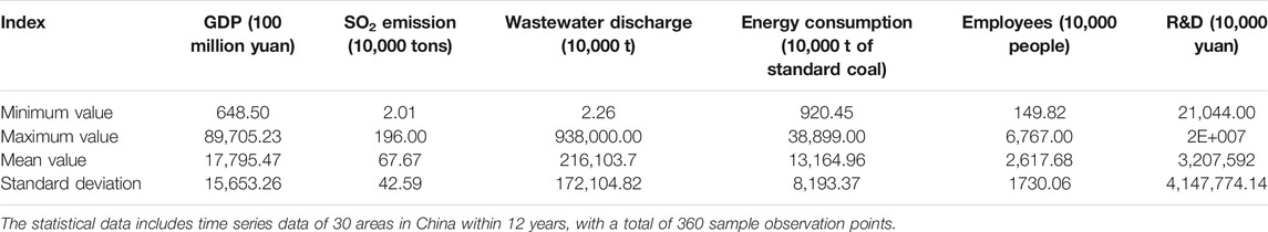
TABLE 1. Data characteristics of low-carbon efficiency input–output indexes.

In the last several years, the DEA model has been used in the research of various fields such as the following: in calculation of the degree of efficiency in productivity (Matas, 1998; Lambert, 1999; Lovell, 2003; Mussard and Peypoch, 2006; Charles et al., 2012; Fancello et al., 2014), ecological efficiency (Le Lannier and Porcher, 2014; Wang et al., 2014; Deilmann et al., 2016; Gudipudi et al., 2018), and economic efficiency (Li et al., 2017; Ruiz Estrada et al., 2018). In order to incorporate environmental pollution variables into the DEA model, it is necessary to build a production possibility set containing both “bad” and “good” outputs. Suppose N inputs per area to get M “good” output and I “bad” output. Using x, b, and y to denote input, “bad” output, and “good” output:

$x=\left(x_1,x_2,\mathrm{...},x_N\right)\in R_{+}^N$

$y=\left(y_1,y_2,\mathrm{...},y_M\right)\in R_{+}^M$

$b=\left(b_1,b_2,\mathrm{...},b_M\right)\in R_{+}^I$

P(x) represents the production feasibility set: $P\left(x\right)=\{\left(y,b\right):x$_{can produce} $\left(y,b\right)\},x\in R_{+}^M$. Assuming that P (x) is a convex and closed set, the input x and the “good” output y can be freely disposed (Fare and Primont, 1995). If P (x) satisfies the conditions Weak Disposability and Null-jointness of Outputs, P (x) can be used to represent environmental efficiency. Null-jointness is also known as Byproducts Axiom, which means that the “bad” output must appear with the “good” output; Weak Disposability of Outputs means “bad” output, and “good” outputs are concentrated in production feasibility, but the same proportion decreases. It means that the “good” output must decrease as the “bad” output decreases and increase as it increases (Fare and Grossk, 2007).

The function of the DEA-Malmquist index is to measure the growth rate of the environmental efficiency of each region. The calculation methods of total factor productivity include parametric and nonparametric methods (Banker, 1984; Arellano and Bond, 1991). In recent years, a lot of studies have used the BCC and Charnes et al. (1978) proposed Charnes Cooper and Rhodes (CCR) analysis methods of the DEA-Malmquist model to calculate the environmental efficiency (Goto et al., 2014; Sueyoshi and Goto, 2014; Lorenzo-Toja et al., 2015; Sueyoshi and Yuan, 2017; Guo et al., 2020). Scheel (2001) pointed out that in the production process, various environmental pollutants will inevitably be produced, which cannot meet the traditional DEA efficiency model’s assumption about “maximizing output,” and the undesired output needs to be considered adding into the traditional DEA model. The use of the nonparametric DEA-Malmquist index model to study the rate of rise of the environmental efficiency index is relatively lacking. In 1953, Malmquist proposed the Malmquist index method (Grifell-Tatje and Lovell, 1995). The Malmquist index has been widely used in various fields. It can measure productivity changes under dynamic settings. When using the Malmquist index to evaluate production efficiency, the factors that influence the change in production efficiency can also be discussed, such as the impact of changes in scale and technological progress. Simar and Wilson (2019) extended the previous results and developed a new central limit theorem that was used to infer the geometric mean of the subindex of the original data and the arithmetic mean of the log of the subindex. Pastor et al. (2020) said that there is no research on the traditional Malmquist index as total factor productivity (TFP) index at present. He proposed a new Malmquist exponential decomposition method based on the “scale constant return” proportional direction distance function (pDDF) and expressed the change in production efficiency as the change caused by two influencing factors, namely, the variety in production efficiency and the denominator caused by the difference in molecular output changes in production efficiency caused by input changes.

At the same time, the nonparametric linear programming method was combined with the DEA model, which resulted into the development of the DEA-Malmquist model that is used to compute the ratio between outputs and inputs at different times. In recent years, the DEA-Malmquist index method has been gradually used in the research of various fields such as in court reform (Falavigna et al., 2018), in healthcare (Prior, 2006; Fragkiadakis et al., 2016; Bastian et al., 2016), and in energy efficiency (Huang et al., 2017; Fernández et al., 2018; Mavi and Mavi, 2019). Li et al. (2017) selected data from 742 listed Chinese companies and used the cross-sectional DEA-Malmquist model to predict the financial difficulties of the listed companies. Furthermore, by using the time-varying Malmquist-DEA, the competitive position of the listed companies was dynamically predicted. The Malmquist-DEA model can intelligently adjust the efficiency boundary and make reliable predictions over time. Wang (2019) selected 40 global cities from 2012 to 2018 as samples and evaluated urban globalization performance efficiency from six aspects: economy, culture, environment, and research and development based on the DEA model. Then, he derived the DEA-Malmquist index and tracked the reasons for its performance efficiency changes. Chen et al. (2020) used the DEA model to measure the evolution of the destocking performance of the industry in China from 2005 to 2015. This is the first time that the DEA-Malmquist model has been applied to the real estate industry. Due to decision-making units (DMUs’) destocking efficiency, regional differences in input redundancy, and total inventory, no policy can fully and effectively affect all regions and solve problems. The measures affecting production efficiency should be changed according to the specific situation.

This paper takes 30 regions of China as research samples, uses the DEA model to measure the growth rate of environmental efficiency from 2006 to 2017, and conducts an empirical research on the factors that affect the growth rate.

The principle of mathematical programming is the basis of the DEA model, using multiple sets of expenditures and combined data to obtain production efficiency, as depicted in Figure 1. The number of DMUs is N, and each DMU has K inputs and M outputs. The input and output of DMU_i are represented by column vectors x_i and y_i, respectively. In this way, under the conditions of closed convex technology, fixed scale return (C), and strong disposal of input factors (S), the CRS-DEA method is input-oriented. It can be obtained by solving linear programming (LP):

$D\left(y_i,x_i\right)=Min\theta ,st-y_i+Y\lambda \ge 0,\theta x_i-X\lambda \ge 0,\lambda \ge 0$

FIGURE 1

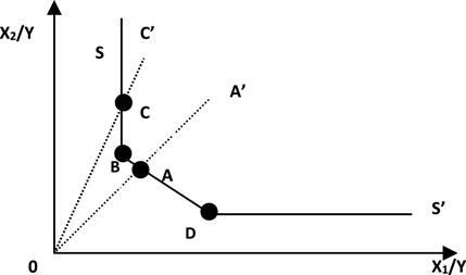
FIGURE 1. Illustration of DEA efficiency.

DMUs with θ = 1 are at the production frontier of best practices. DMUs with θ < 1 are inefficient. They can be projected to the front by reducing the input to (1-θ)x_i along the ray direction. This adjustment is called radial adjustment.

In the “piecewise” linear form of the DEA’s nonparametric front, when the current edge is parallel to the number axis, it will produce an input slack problem.

As shown in Figure 1, the maximum output Y on the frontier of production is standardized as 1, and the inputs of X₁ and X₂ are divided by Y to standardize. The input–output combination of B and D forms the frontier. The input–output combination of A′ and C′ is inefficient. A′ can be adjusted to the production front A through the ray AA′. However, because the production Frontier is a piecewise linear form, after the C′ adjusts to the production Frontier C through the ray CC’. Furthermore, we can reduce the input X2 of the CB quantity to retain it on the production frontier. The adjustment of the input elements along the production frontier is called slack adjustment.

The DEA model measures the distance from each DMU to the production frontier boundary and quantifies it between 0 and 1. For example, a DMU located at or above the production frontier boundary is considered to be effective and is assigned a value of 1, while a DMU located below the production frontier boundary is considered insufficiently efficient and the efficiency score is less than 1. The DEA model has three advantages. First, the DEA model does not need to demonstrate in advance whether input factors are the inevitable cause of output factors. When there is no way to describe and summarize the production process, the DEA model is suitable. Second, the DEA model can select multiple input and output indicators. Finally, unlike the absolute value of the efficiency calculated by the AHP model, the DEA model calculates the relative efficiency value, which is particularly suitable for ranking multiple DMUs.

Then, scholars developed various DEA models to meet the demand under various situations. Charnes et al. (1978) proposed CCR, which was an efficiency measurement method based on the precondition of constant returns to scale. If convexity constraints are added into the CCR model, we can get the BCC model, which can distinguish between pure technical efficiency and scale efficiency in technical efficiency.

According to the traditional DEA model, the efficiency values of each sample area in two periods are in different benchmarking periods and cannot be directly compared. The Malmquist index can calculate the production efficiency in different periods. Therefore, the DEA-Malmquist model is an analysis method that combines the concept of the Malmquist index with the DEA model.

The basic idea of the DEA-Malmquist index method is to assume that in each year $t=\mathrm{1,2},\mathrm{...},T$, the input-–output value of the K province is $\left(x^{k,t},y^{k,t},b^{k,t}\right)$. On the basis of meeting the above conditions, there are

$P^t\left(x^t\right)=\left\{\left(y^t,b^t\right):{\displaystyle \sum _{K=1}^K{Z}_k^t{x}_{kn}^t\le x_{kn}^t,n=1,\mathrm{...},N};{\displaystyle \sum _{k=1}^k{z}_k^t{y}_{km}^t\ge y_{km}^t,m=1,\mathrm{...},M};{\displaystyle \sum _{k=1}^k{z}_k^t{b}_{ki}^t=b_{ki}^t,i=1,\mathrm{...},I;z_k^t\ge 0,k=1,\mathrm{...},K}\right\}$

The technical index reference value for year t can be expressed as ${\overline{P}}^t\left(x\right)=\left\{y:y\le z{\overline{Y}}^t,x\ge z{\overline{X}}^t,z\ge 0\right\}$, ${\overline{X}}^t=\left(\cdots ,X^{t_0},\cdots X^{t-1},X^t\right)$, and ${\overline{Y}}^t=\left(\cdots ,Y^{t_0},\cdots Y^{t-1},Y^t\right)$, where $z$ denotes the weight of the observed value of the cross section in every DMU. In the calculation, the indicator values of year $t_0$ and all previous years need to be used. However, it is difficult to obtain the value of the indicator before $t_0$. Therefore, the technical index reference value for year t is expressed as

${\overline{P}}^t\left(x/{\overline{X}}^{t_0}=X^{t_0},{\overline{Y}}^{t_0}=Y^{t_0}\right)=\left\{y:y\le z\left(Y^{t_0},\cdots ,Y^{t-1},Y^t\right),x\ge z\left(X^{t_0},\cdots ,X^{t-1},X^t\right),z\ge 0\right\}$ At this time, the distance function of each province in year t is $d^t\left(x^t,y^t\right)=\inf \left\{\theta :\left(x^t,y^t/\theta \right)\in {\overline{P}}^t\right\}$, where $d^t\left(x^t,y^t\right)=1$ indicates that the input–output value of year t is on the production boundary, showing efficiency, and $d^t\left(x^t,y^t\right)>1$ indicates that the input–output value of year t is within the production boundary, showing inefficiency.

At this time, the Malmquist index is expressed as $M_0^t=d^{t+1}\left(x^{t+1},y^{t+1}\right)/d^t\left(x^t,y^t\right)$. Further, it is decomposed into changes in technological progress and changes in technological efficiency:

$\text{TFP}=\text{TECH∗EFF}=\text{TECH∗PE∗SE}$

Among them, TFP is the change in environmental efficiency; TECH is the change in technological progress which depends on the impact of boundary transfers. EFF represents the change of technical efficiency which presents the efficiency change of the same DMU in different periods based on the benchmark test to get to the border. PE is the change of pure technical efficiency. SE is the change of scale efficiency.

In order to better clarify the connotation of TECH and EFF, we use a simple input-oriented example (two inputs and one output) to illustrate the DEA-Malmquist model used in this article. In Figure 2, the two axes represent two inputs and one output. Suppose (E) and (H) are the positions of DMU in year t and year t + n. The two piecewise linear curves represent the production frontier boundary at year t and year t + n. The projections of (E) on the two curves are (F) and (G). Similarly, the projections of (H) on the two curves are (I) and (J). The DEA efficiency of (E) at t can be shown as OE/OF. The DEA efficiency of (E) at t + n can be expressed as OE/OG. Similarly, the DEA efficiency of (H) at time t can be expressed as OH/OI. The DEA efficiency of (H) at t + n can be expressed as OH/OJ. The DEA-Malmquist value is

$\sqrt{\frac{\frac{OE}{OF}\times \frac{OE}{OG}}{\frac{OH}{OI}\times \frac{OH}{OJ}}}=\frac{\frac{OE}{OF}}{\frac{OH}{OI}}\times \sqrt{\frac{\frac{OH}{OI}\times \frac{OE}{OG}}{\frac{OE}{OF}\times \frac{OH}{OJ}}}=\frac{\frac{OE}{OF}}{\frac{OH}{OI}}\times \sqrt{\frac{OI}{OJ}\times \frac{OF}{OG}}=TECH\times EFF$

FIGURE 2

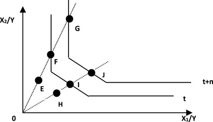
FIGURE 2. Illustration of the DEA-Malmquist model.

$\frac{\frac{OE}{OF}}{\frac{OH}{OI}}$ _{stands for EFF, determined by the overall characteristics and performance of the DMU itself.} $\sqrt{\frac{OI}{OJ}\times \frac{OF}{OG}}$ _{stands for TECH, which shows the impact of changes in production boundaries.}

Analysis

This paper uses DEAP 2.1, VRS (based on returns to scale), and the input-oriented DEA model to calculate and decompose the environmental efficiency of 30 areas in China from 2006 to 2017.

The Average Growth Rate of China’s Environmental Efficiency

In Table 2, this paper shows that the average growth rate of China’s environmental efficiency index from 2006 to 2017 was 1.045, and the overall growth rate was 4.5%. For each of the years, only 2008–2009 and 2010–2011 showed a negative growth, −2.5% and −8.1%, respectively, and the other years showed a positive growth. The reason for this may be that in recent years, the central government has improved the governance methods of environmental protection continuously, and environmental legislation has been gradually improved. Each region has committed great importance to “environmental governance.” The ecological civilization reform has become one of the “five tasks,” and “environmental governance” has become a long-term trend rather than a short-term boom. Therefore, the overall growth rate of the environmental efficiency index also shows a positive growth trend.

TABLE 2

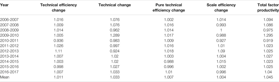
TABLE 2. China’s environmental efficiency change.

From the decomposition of the growth rate of the environmental efficiency index, the environmental technological efficiency and technological progress are increased slightly; the amplitudes are 1.1% and 3.3% in China, respectively, indicating that both the development of technological efficiency and progress are conducive to promoting the growth of environmental efficiency, of which the contribution of technological progress is even greater. Figure 3 shows, from 2009 to 2010, the growth rate of TFP reached 29.5%, of which the technical change reached 28.9%, which is due to the “The Stockholm Convention on Persistent Organic Pollutants (POPs)” in May 2009. The corresponding amendments came into force on August 26, 2010. During this period, in order to improve stakeholders’ understanding of the content and mechanism of the Convention and promote the implementation of follow-up work, in July 2010, the United Nations Environment Programme held an international seminar, which greatly promoted the environmental efficiency.

FIGURE 3

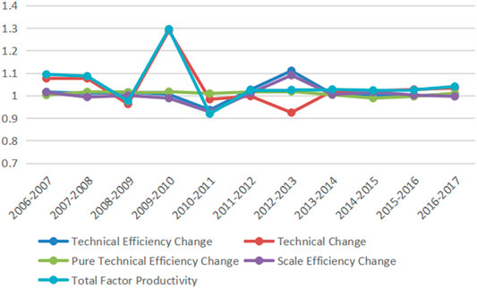
FIGURE 3. Movement track of China’s environmental efficiency change.

Further decomposing the changes in pure technology scale and efficiency, it can be found that pure technology efficiency has maintained a stable positive growth for a long time, and there was only a small negative growth between 2014 and 2016. The scale efficiency showed a fluctuant trend, indicating that the adjustment of industrial structure, promoting the development of high new technology, and other measures have obtained a certain effect in China.

Interprovincial Heterogeneity of Changes in China’s Environmental Efficiency Index

According to China’s improvement of the level of economic and social development in China, 30 areas are divided into three major areas: eastern, central, and western.

Table 3 shows a further situation of changes in the environmental efficiency index and its decomposition. The growth rate of China’s environmental efficiency index was 4.5% from 2006 to 2017. The average changes in the environmental efficiency of the eastern, western, and central areas showed positive growth, and most of the provinces and cities are on the increase. On the space layout, a trend has been presented, showing that the average changes in central regions exceed those in eastern regions. In western areas, the average changes are lower than those in eastern and central areas.

TABLE 3

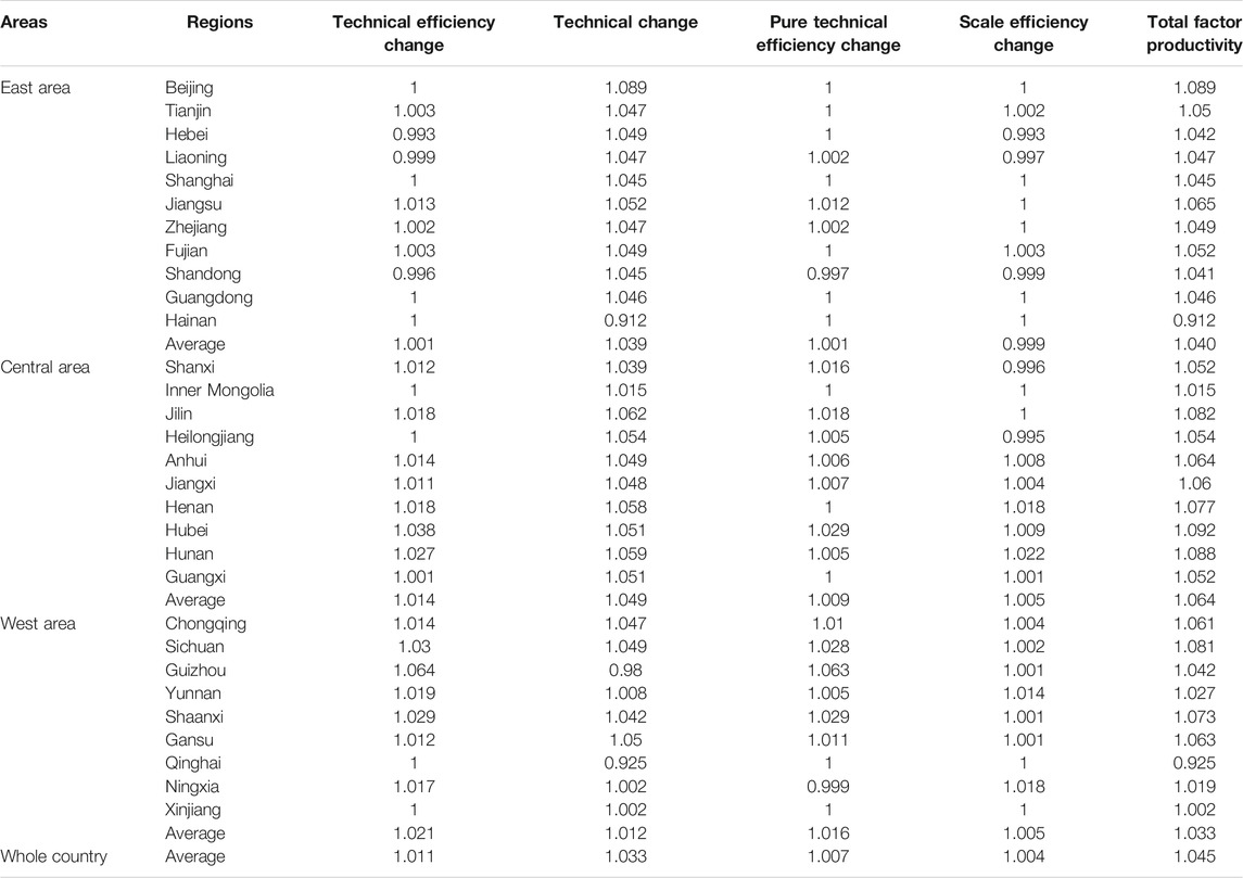
TABLE 3. China’s regional environmental efficiency change from 2006 to 2017.

Eastern Areas

Eastern areas include 11 areas which are Beijing, Tianjin, Jiangsu, Hebei, Liaoning, Guangdong, Shanghai, Zhejiang, Fujian, Shandong, and Hainan. With the exception of Hainan, the environmental efficiency indexes of all provinces and cities showed positive growth. Among them, Beijing has the highest growth rate of 8.9%. This is because in recent years, Beijing has vigorously promoted the optimization of energy structure and the adjustment of regional industrial structures. It has implemented energy consumption by replacing coal with gas or electricity to control total coal consumption. A series of practicable measures such as optimizing regional transportation structure, increasing railway transportation volume, and reducing road diesel vehicle transportation volume are implemented. Especially in the implementation of “Enhanced Measures for the Prevention and Control of Air Pollution in the Beijing-Tianjin-Hebei Region (2016-2017),” and “Water Pollution Control Action Plan,” the air quality continued to improve, and the sewage treatment rate was 92%. According to the “2017 Beijing Environmental Status Bulletin,” Beijing has achieved continuous improvement in air quality through 5 years of governance. Hainan’s environmental efficiency index showed a negative growth of −8.8%. This is because Hainan has a unique geographical location and natural conditions, and its main development is tourism and modern service industries. In addition to that, its environmental efficiency reached the production frontier between 2006 and 2017 so there is less room for improvement in environmental efficiency. The growth rate of the DEA-Malmquist environmental efficiency index is a dynamic indicator, so there is little room for growth in environmental efficiency in Hainan.

Central Areas

Central areas include 10 areas which are Shanxi, Inner Mongolia, Hubei, Jilin, Heilongjiang, Jiangxi, Anhui, Henan, Hunan, and Guangxi. The environmental efficiency indexes of all central areas are increasing, and the average growth rate is 6.4%. This is because the central provinces have combined the advantages of various regions and adopted the green development path of characteristic development and dislocation development since the 18th National Congress of the Communist Party. It also focused on cultivating and developing the endogenous driving force of the green economy. They have formed the advantages of protection during development and development during protection. Recently, the central provinces have turned the improvement of environmental efficiency into specific ecological civilization practices. For example, some provinces have comprehensively implemented the five-level river chief, lake chief, and forest chief system. It will cover ecological compensation of the whole river basin, taking the lead in carrying out the pilot reform of comprehensive enforcement. Among them, Hubei has the highest growth rate of 9.2%. This is because under the guidance of “Outline of the Yangtze River Economic Belt Development Plan” and “Ecological Environment Protection Plan of the Yangtze River Economic Belt,” Hubei Province has formulated the corresponding five special plans based on these policy measures. These plans have formulated strict rectification or improvement plans for the chemical industry and iron industry along the Yangtze River, as well as a timetable and roadmap for relocation into the industrial park, so as to make the industrial structure and optimization of framework in the industry of the Yangtze River ecological safety go on wheels.

Western Areas

Western areas include nine areas which include Sichuan, Qinghai, Chongqing, Guizhou, Shaanxi, Yunnan, Gansu, Ningxia, and Xinjiang. Except Qinghai, all areas have positive growth in environmental efficiency indexes. Among them, Sichuan has the highest growth rate of 8.1%. This is because Sichuan’s environmental supervision and enforcement have been very effective. In 2017 alone, the province levied a total of 753 million Yuan in sewage charges and installed 2,894 automatic monitoring facilities for key sewage enterprises. In addition, the former Ministry of Environmental Protection established the Southwest Regional Air Quality Forecasting and Forecasting Center in Sichuan Province to carry out comprehensive air quality forecasting and forecasting work. From the aspect of spatial distribution, the environmental efficiency index of western China has the lowest growth rate. This is because the proportion of counties that have been evaluated as “comparatively poor” and “poor” in China’s ecological environment reached 32.9%, and these areas are largely due to northwestern areas, such as the northern Qinghai-Tibet Plateau, Gansu, and most of Xinjiang (according to the “Technical Specifications for the Evaluation of the Ecological Environment Status”). Environmental management in these areas is difficult.

From a static perspective Table 4 shows, the average value of China’s environmental efficiency in 2017 was 0.887, which was less than 1. The mean efficiency of pure technology is 0.936, and the mean efficiency of scale technology is 0.948. Eleven provinces and cities reached the frontier of production. Except for Anhui and Chongqing, which showed diminishing returns to scale, the other 17 provinces and cities all showed increasing returns to scale. Among them, Hebei, Jiangxi, Henan, and Guangxi had a pure technical efficiency of 1. Environmental efficiency can be improved by increasing investment.

TABLE 4

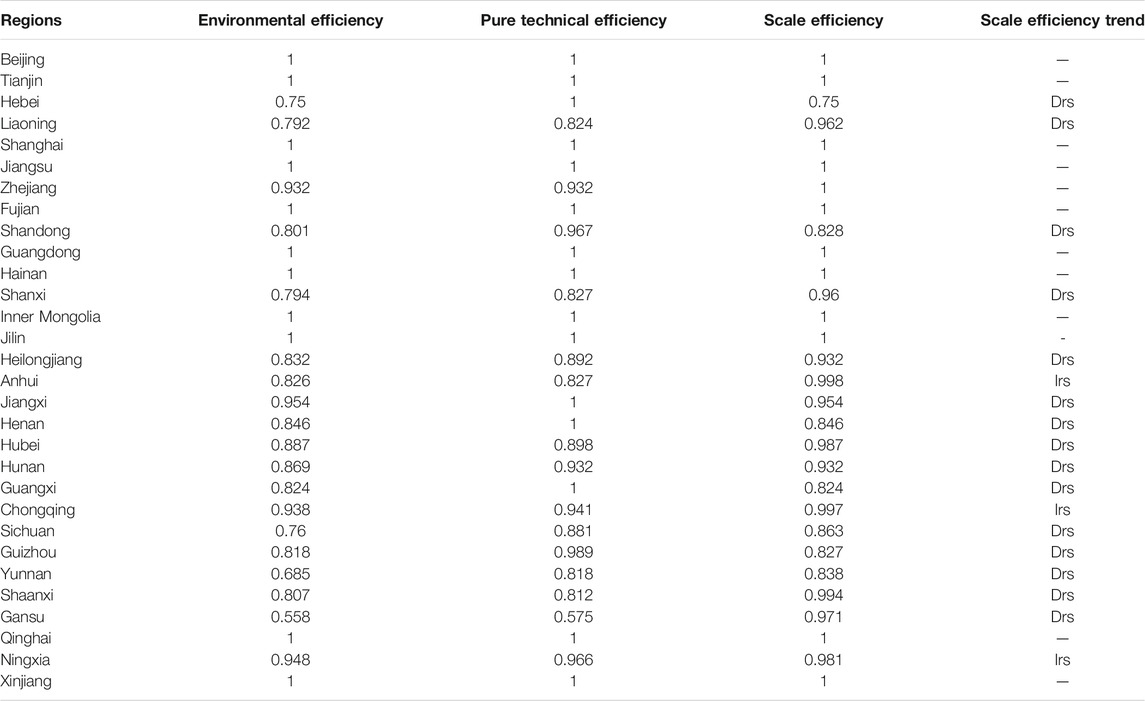
TABLE 4. China’s regional environmental efficiency in 2017.

Analysis of Influencing Factors of China’s Environmental Efficiency Index

There are many factors that affect environmental efficiency. We use panel data of 30 areas from 2006 to 2017 to find out the main influencing factors of environmental efficiency. With reference to influencing factors which are frequently used in relevant typical studies of authoritative institutions, the factors of government intervention, the output value of the tertiary industry, the level of urbanization, the average length of education of residents, and the protection of intellectual property rights are analyzed (in Table 5).

TABLE 5

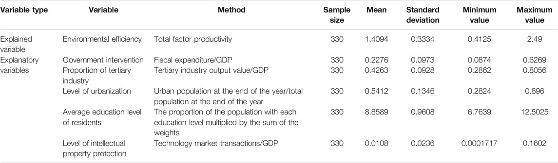
TABLE 5. Descriptive statistics.

Firstly, it is government intervention (GOV). In China, the basis for the decentralization between the local and central governments is not strictly divided according to the spillover scope of public goods. Under the shelter of “local protectionism,” environmental law enforcement often falls into the cycle of “pollution, investigation, and fines” (Shi Qingling Chen Shiyi, Guo Feng, 2017). It is generally believed that the strength of government financial support plays a crucial role in improving environmental efficiency.

Secondly, it is the proportion of the tertiary industry’s value of outputs in GDP and the level of urbanization (CIT). Structural factors are important factors affecting environmental efficiency. It is generally believed that with the increase in the proportion of industry in the national economy, the degree of pollution to the environment will increase accordingly. Therefore, changing the industrial structure can improve low-carbon efficiency. The process of urbanization has caused serious difficulties in supporting natural resources. To ensure the rational use of resources in urbanization development, it is inevitable to increase environmental efficiency.

Thirdly, it is “years of education for residents” (EDU). Peoples’ awareness of environmental protection is very important for improving environmental efficiency. It is mainly cultivated from an early age and has a close relationship with education.

Finally, there is the protection of intellectual property rights (KNO). At present, China is vigorously giving impetus to innovation of clean and renewable energy technologies. Technological progress factors also promote environmental efficiency. According to intellectual property theory, strengthening intellectual property protection is conducive to fairness in the environmental protection market and promotes technological competition, thereby resulting into improving environmental efficiency.

Building the following model:

${\mathrm{Y}}_{it}={\beta }_0+{\beta }_{1}GO{V}_{it}+{\beta }_{2}CI{T}_{it}+{\beta }_{3}ED{U}_{it}+{\beta }_{4}KN{O}_{it}+{\epsilon }_{it}$

It should be noted that the growth rate of the environmental efficiency index obtained above is not a static absolute value, so the TFP in 2006 is set to 1, and then the index measured by DEA-Malmquist is converted in a cumulative manner, as the relative level of environmental efficiency each year (Li and Dewan, 2017).

Because the use of OLS calculation will cause the parameter estimates to be biased, this paper uses a restricted dependent variable model, tobit model, for regression analysis, and uses EViews 10 software to calculate the impact of each independent variable on regional environmental efficiency. It indicated that the regional environmental efficiency and GOV showed a significant negative correlation at 5%. The urbanization level showed a significant negative correlation at 1%, and the average education age of resident showed a significant positive correlation at 1% (in Table 6).

TABLE 6

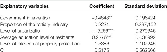
TABLE 6. Regression results based on the Tobit model.

The regression coefficient of the degree of government intervention and regional environmental efficiency is negative and significant at 0.05. In recent years, in order to develop the regional economy and obtain more liquid capital, the phenomenon of lowering environmental standards, “free-riding,” and “race to the bottom” has long existed. Environmental efficiency is used to measure the distance of a region’s pollution emissions from the minimum pollution emissions under the same input and output conditions. The pursuit is to reduce pollution emissions without reducing the speed of economic growth. However, the reality is that the assessment of local governments is more based on the evaluation of economic performance. Therefore, from the perspective of fiscal expenditure, fiscal expenditures of local governments are more favored for productive projects with good economic benefits and more tax revenues, but they ignore the expenditure on environmental pollution. So the higher the level of local government intervention is, the lower the level of development of environmental efficiency is.

The regression coefficient of the tertiary industry proportion and regional environmental efficiency is positive. It can be seen where the tertiary industry occupies a relatively large proportion, the higher the environmental efficiency is. The same is true in China.

The regression coefficient of urbanization level and regional environmental efficiency is negative and significant at 1%. This is because the higher the level of urbanization is, the relatively concentrated the population and industry are, which will generate a large amount of pollutant emissions and reduce the environmental efficiency of that region.

The regression coefficient of EDU and regional environmental efficiency is positive and significant at 0.01. Generally, the higher the education level is, the higher the awareness and the popularity of education among its citizens are, which is good for cutting down pollutant emissions in life and production, thereby increasing the environmental efficiency value of the area.

The regression coefficient of KNO and regional environmental efficiency is positive. This is because the regions with higher intellectual property protection have higher levels of high-tech development, which can effectively promote the development of environmental protection technologies, thereby increasing the environmental efficiency value in that region. China has a vast territory, and there are great differences in resource endowment and industrial economic structure in different regions. Reasonable policy design needs to reflect industry and regional characteristics. Different regions set carbon emission reduction targets in line with local characteristics. At the same time, it should be consistent with China’s overall carbon emission reduction target.

Conclusion

We use panel data of the 30 areas in China from 2006 to 2017 and uses the DEA-Malmquist method to calculate the environmental efficiency of various areas. The Tobit model was constructed to test the factors which are influencing environmental efficiency. The main research conclusions of this article are as follows:

Firstly, from a dynamic perspective, China’s average environmental efficiency index from 2006 to 2017 increased by 4.5%. The average changes in environmental efficiency in the central, eastern, and western areas all illustrated positive growth, and environmental efficiency indexes of most provinces and cities also showed positive growth. From the perspective of spatial layout, there is a tendency that the central areas have a slight advantage compared with the eastern areas, and the eastern areas slightly outdo the western areas. From a static perspective, as of 2017, the average regional environmental efficiency in China was 0.887, which has not yet reached the production frontier. The average value of pure technology efficiency is 0.936, and the average value of scale efficiency is 0.948. Therefore, there is room for improvement from the technological perspective and striving for scale efficiency. In 2017, the environmental efficiency of 11 provinces and cities reached the frontier of production. Except for Anhui and Chongqing, which showed diminishing returns to scale, the other 17 provinces and cities all showed increasing returns to scale. Among them, Hebei, Jiangxi, Henan, and Guangxi’s pure technical efficiency is 1.

Secondly, the influencing factors affecting regional environmental efficiency are further analyzed through the Tobit method, and the results showed that the government intervention and urbanization levels significantly inhibit the regional environmental efficiency. Increasing the average education years of residents significantly promotes regional environmental efficiency. The regression coefficient of tertiary industry proportion and intellectual property protection is positive, but it failed the significance test, and it is not yet possible to determine whether it has significantly promoted regional environmental efficiency or not.

Based on the above analysis, the following information is obtained.

First, to improve China’s ecological environment continuously, we need to lay a solid and stable foundation. As a whole, China’s environmental efficiency and its performance are gradually increasing, but the results are not solid. In the short term, environmental efficiency still shows a fluctuant trend. It may be repeated with a little slack. Environmental efficiency’s steady increase is extremely hard. In order to enhance people’s happiness and build a “Beautiful China,” we need to do the basic work well, improve and upgrade industrial structures, promote cleaner production, increase policy support for environmental protection industry development, and improve environmental efficiency in a sustainable manner.

Second, it is essential to learn from effective experience, better explore the local advantages of various regions, and take the path of green economic development, such as characteristic development and dislocation development. Although from the static time point of view, the environmental efficiency of the eastern areas was in the leading state in 2017, it is worth noting that the central areas have developed rapidly in the past decade. The average environmental efficiency indexes of all provinces and municipalities in the central region between 2006 and 2017 are all growing positively. The average growth rate reaches 6.4%, which is higher than the growth rate in the eastern region. We should fully study and learn from the green development practices of the central provinces, strive to find our own regional advantages, and form an endogenous drive of protection during development and during protection. Accelerating new industrialization, informatization, urbanization, and agricultural modernization is the phase that China, as a developing country, is still in. The foundation for achieving comprehensive green transformation is still weak. The foundation for achieving a comprehensive green transformation is still weak, and the pressure on ecological and environmental protection has not been radically relieved. Yet, new industries and business models will be accomplished step by step in the process of achieving the “dual-carbon” goal. China should fit the trend of technological revolution and industrial transformation, look for opportunities brought by green transformation, and seek development opportunities from green development. If China feels like boosting carbon peaking and carbon neutrality, it ought to follow the way of source prevention, industrial adjustment, technological innovation, and green life; speed up the realization of green transformation in production and way of life; and promote the realization of the “dual-carbon” goal on time.

Data Availability Statement

The original contributions presented in the study are included in the article/Supplementary Material; further inquiries can be directed to the corresponding author.

Author Contributions

All authors listed have made a substantial, direct, and intellectual contribution to the work and approved it for publication.

Funding

This work is supported by the Ministry of Education of Humanities and Social Science Project of China (21YJC630104) and the National Natural Sciences Foundation of China (72172112).

Conflict of Interest

The authors declare that the research was conducted in the absence of any commercial or financial relationships that could be construed as a potential conflict of interest.

Publisher’s Note

All claims expressed in this article are solely those of the authors and do not necessarily represent those of their affiliated organizations, or those of the publisher, the editors and the reviewers. Any product that may be evaluated in this article, or claim that may be made by its manufacturer, is not guaranteed or endorsed by the publisher.

References

Andrew, A. A., Tomiwa, S. A., and Stephen, T. O. (2021). Examining the Dynamics of Ecological Footprint in China With Spectral Granger Causality and Quantile-On-Quantile Approaches. Int. J. Sustainable Development World Ecol., 1–14. doi:10.1080/13504509.2021.1990158

CrossRef Full Text | Google Scholar

Arellano, M., and Bond, S. (1991). Some Tests of Specification for Panel Data: Monte Carlo Evidence and an Application to Employment Equations. Rev. Econ. Stud. 58, 277–297. doi:10.2307/2297968

CrossRef Full Text | Google Scholar

Banker, R. D. (1984). Estimating Most Productive Scale Size Using Data Envelopment Analysis. Eur. J. Oper. Res. 17 (1), 35–44. doi:10.1016/0377-2217(84)90006-7

CrossRef Full Text | Google Scholar

Bastian, N. D., Kang, H., Swenson, E. R., Fulton, L. V., and Griffin, P. M. (2016). Evaluating the Impact of Hospital Efficiency on Wellness in the Military Health System. Mil. Med. 181 (8), 827–834. doi:10.7205/milmed-d-15-00309

PubMed Abstract | CrossRef Full Text | Google Scholar

Charles, V., Kumar, M., and Irene Kavitha, S. (2012). Measuring the Efficiency of Assembled Printed Circuit Boards With Undesirable Outputs Using Data Envelopment Analysis. Int. J. Prod. Econ. 136 (1), 194–206. doi:10.1016/j.ijpe.2011.11.010

CrossRef Full Text | Google Scholar

Charnes, A., Cooper, W. W., and Rhodes, E. (1978). Measuring the Efficiency of Decision Making Units. Eur. J. Oper. Res. 2, 429–444. doi:10.1016/0377-2217(78)90138-8

CrossRef Full Text | Google Scholar

Chen, K., Song, Y.-y., Pan, J.-f., and Yang, G.-l. (2020). Measuring Destocking Performance of the Chinese Real Estate Industry: A DEA-Malmquist Approach. Socio-Economic Plann. Sci. 69 (3), 100691. doi:10.1016/j.seps.2019.02.006

CrossRef Full Text | Google Scholar

Deilmann, C., Lehmann, I., Reißmann, D., and Hennersdorf, J. (2016). Data Envelopment Analysis of Cities - Investigation of the Ecological and Economic Efficiency of Cities Using a Benchmarking Concept From Production Management. Ecol. Indicators. 67, 798–806. doi:10.1016/j.ecolind.2016.03.039

CrossRef Full Text | Google Scholar

Dimitra, K., and Efthimios, Z. (2013). The Environmental Kuznets Curve (EKC) Theory-Part A: Concept, Causes and the CO2 Emissions Case. Energy Policy. 62 (11), 1392–1402. doi:10.1016/j.enpol.2013.07.131

CrossRef Full Text | Google Scholar

Falavigna, G., Ippoliti, R., and Ramello, G. B. (2018). DEA-Based Malmquist Productivity Indexes for Understanding Courts Reform. Socio-Economic Plann. Sci. 62 (7), 31–43. doi:10.1016/j.seps.2017.07.001

CrossRef Full Text | Google Scholar

Fancello, G., Uccheddu, B., and Fadda, P. (2014). Data Envelopment Analysis (D.E.A.) for Urban Road System Performance Assessment. Proced. - Soc. Behav. Sci. 111, 780–789. doi:10.1016/j.sbspro.2014.01.112

CrossRef Full Text | Google Scholar

Fare, R., Grosskopf, S., and Pasurkajr, C. (2007). Environmental Production Functions and Environmental Directional Distance Functions. Energy. 32, 1055–1066. doi:10.1016/j.energy.2006.09.005

CrossRef Full Text | Google Scholar

Fare, R., and Primont, D. (1995). Multi-output Production and Duality:Theory and Applications, 3. Boston: Kluwer Academic Publishers, 46–90.

Google Scholar

Fernández, D., Pozo, C., Folgado, R., Jiménez, L., and Guillén-Gosálbez, G. (2018). Productivity and Energy Efficiency Assessment of Existing Industrial Gases Facilities via Data Envelopment Analysis and the Malmquist index. Appl. Energ. 212 (15), 1563–1577. doi:10.1016/j.apenergy.2017.12.008

CrossRef Full Text | Google Scholar

Fragkiadakis, G., Doumpos, M., Zopounidis, C., and Germain, C. (2016). Operational and Economic Efficiency Analysis of Public Hospitals in Greece. Ann. Operations Res. 247, 787–806. doi:10.1007/s10479-014-1710-7

CrossRef Full Text | Google Scholar

Goto, M., Otsuka, A., and Sueyoshi, T. (2014). DEA (Data Envelopment Analysis) Assessment of Operational and Environmental Efficiencies on Japanese Regional Industries. Energy. 66 (1), 535–549. doi:10.1016/j.energy.2013.12.020

CrossRef Full Text | Google Scholar

Grifell-Tatjé, E., and Lovell, C. A. K. (1995). A Note on the Malmquist Productivity index. Econ. Lett. 47 (2), 169–175. doi:10.1016/0165-1765(94)00497-p

CrossRef Full Text | Google Scholar

Gudipudi, R., Lüdeke, M. K. B., Rybski, D., and Kropp, J. P. (2018). Benchmarking Urban Eco-Efficiency and Urbanites' Perception. Cities. 74, 109–118. doi:10.1016/j.cities.2017.11.009

CrossRef Full Text | Google Scholar

Guo, Y., Yu, Y., Ren, H., and Xu, L. (2020). Scenario-Based DEA Assessment of Energy-Saving Technological Combinations in Aluminum Industry. J. Clean. Prod. 260 (1), 121010. doi:10.1016/j.jclepro.2020.121010

CrossRef Full Text | Google Scholar

Huang, J., Du, D., and Hao, Y. (2017). The Driving Forces of the Change in China's Energy Intensity: An Empirical Research Using DEA-Malmquist and Spatial Panel Estimations. Econ. Model. 65 (9), 41–50. doi:10.1016/j.econmod.2017.04.027

CrossRef Full Text | Google Scholar

Jack, F., Bruce, M., and Tim, T. (2012). Dynamic Misspecification in the Environmental Kuznets Curve: Evidence From CO2 and SO2 Emissions in the United Kingdom. Ecol. Econ. 76 (4), 25–33. doi:10.1016/j.ecolecon.2012.01.023

CrossRef Full Text | Google Scholar

Lambert, D. K. (1999). Scale and the Malmquist Productivity Index. Appl. Econ. Lett. 6 (9), 593–596. doi:10.1080/135048599352673

CrossRef Full Text | Google Scholar

Lannier, A. L., and Porcher, S. (2014). Efficiency in the Public and Private French Water Utilities: Prospects for Benchmarking. Appl. Econ. 46 (5), 556–572. doi:10.1080/00036846.2013.857002

CrossRef Full Text | Google Scholar

Li, B., and Dewan, H. (2017). Efficiency Differences Among China's Resource-Based Cities and Their Determinants. Resour. Pol. 51, 31–38. doi:10.1016/j.resourpol.2016.11.003

CrossRef Full Text | Google Scholar

Li, Z., Crook, J., and Andreeva, G. (2017). Dynamic Prediction of Financial Distress Using Malmquist DEA. Expert Syst. Appl. 80 (1), 94–106. doi:10.1016/j.eswa.2017.03.017

CrossRef Full Text | Google Scholar

Lorenzo-Toja, Y., Vázquez-Rowe, L., Vázquez-Rowe, I., Chenel, S., Marín-Navarro, D., Moreira, M. T., et al. (2015). Eco-Efficiency Analysis of Spanish WWTPs Using the LCA + DEA Method. Water Res. 68 (1), 651–666. doi:10.1016/j.watres.2014.10.040

PubMed Abstract | CrossRef Full Text | Google Scholar

Lovell, C. A. K. (2003). The Decomposition of Malmquist Productivity Indexes. J. Prod. Anal. 20 (3), 437–458. doi:10.1023/a:1027312102834

CrossRef Full Text | Google Scholar

Luis, A., Guadalupe, A., Tobias, K., and Joao, F. (2018). Trade from Resource-Rich Countries Avoids the Existence of a Global Pollution Haven Hypothesis. J. Clean. Prod. 175 (2), 599–611. doi:10.1016/j.jclepro.2017.12.056

CrossRef Full Text | Google Scholar

Matas, A., and Raymond, J. L. (1998). Technical Characteristics and Efficiency of Urban Bus Companies: The Case of Spain. Transportation. 25, 243–264. doi:10.1023/a:1005078830008

CrossRef Full Text | Google Scholar

Mavi, N. K., and Mavi, R. K. (2019). Energy and Environmental Efficiency of OECD Countries in the Context of the Circular Economy: Common Weight Analysis for Malmquist Productivity Index. J. Environ. Manage. 247 (1), 651–661. doi:10.1016/j.jenvman.2019.06.069

CrossRef Full Text | Google Scholar

Mussard, S., and Peypoch, N. (2006). On Multi-Decomposition of the Aggregate Malmquist Productivity Index. Econ. Lett. 91 (3), 436–443. doi:10.1016/j.econlet.2006.01.015

CrossRef Full Text | Google Scholar

Nicholars, A., and Ilhan, O. (2015). Testing Environmental Kuznets Curve Hypothesis in Asian Countries. Ecol. Indicators. 52 (5), 16–22. doi:10.1016/j.ecolind.2014.11.026

CrossRef Full Text | Google Scholar

Ozgur, B. S., Tomiwa, S. A., and Dervis, K. (2021). The Imperativeness of Environmental Quality in China Amidst Renewable Energy Consumption and Trade Openness. Sustainability. 13 (9), 5054.

Google Scholar

Pastor, J. T., Lovell, C. A. K., and Aparicio, J. (2020). Defining a New Graph Inefficiency Measure for the Proportional Directional Distance Function and Introducing a New Malmquist Productivity index. Eur. J. Oper. Res. 281 (1), 222–230. doi:10.1016/j.ejor.2019.08.021

CrossRef Full Text | Google Scholar

Pérez, K., González-Araya, M. C., and Iriarte, A. (2017). Energy and GHG Emission Efficiency in the Chilean Manufacturing Industry: Sectoral and Regional Analysis by DEA and Malmquist Indexes. Energ. Econ. 66, 290–302. doi:10.1016/j.eneco.2017.05.022

CrossRef Full Text | Google Scholar

Prior, D. (2006). Efficiency and Total Quality Management in Health Care Organizations: a Dynamic Frontier Approach. Ann. Oper. Res. 145 (1), 281–299. doi:10.1007/s10479-006-0035-6

CrossRef Full Text | Google Scholar

Ruiz Estrada, M. A., Park, D., and Khan, A. (2018). The Impact of Terrorism on Economic Performance: The Case of Turkey. Econ. Anal. Pol. 60, 78–88. doi:10.1016/j.eap.2018.09.008

CrossRef Full Text | Google Scholar

Sakiru, A., Usama, A., Ibrahim, M., and Ilhan, O. (2017). Investigating the Pollution haven Hypothesis in Ghana: An Empirical Investigation. Energy. 124 (4), 706–716. doi:10.1016/j.energy.2017.02.089

CrossRef Full Text | Google Scholar

Scheel, H. (2001). Undesirable Outputs in Efficiency Valuations. Eur. J. Oper. Res. 132 (2), 400–410. doi:10.1016/s0377-2217(00)00160-0

CrossRef Full Text | Google Scholar

Shan, S., Munir, A., Zhixiong., T., Tomiwa, S. A., Rita, Y. M. L., and Dervis, K. (2021). The Role of Energy Prices and Non-linear Fiscal Decentralization in Limiting Carbon Emissions: Tracking Environmental Sustainability. Energy. 234, 121243. doi:10.1016/j.energy.2021.121243

CrossRef Full Text | Google Scholar

Simar, L., and Wilson, P. W. (2019). Central Limit Theorems and Inference for Sources of Productivity Change Measured by Nonparametric Malmquist Indices. Eur. J. Oper. Res. 277 (12), 756–769. doi:10.1016/j.ejor.2019.02.040

CrossRef Full Text | Google Scholar

Soumyananda, D. (2004). Environmental Kuznets Curve Hypothesis: A Survey. Ecol. Econ. 49 (4), 431–455. doi:10.1016/j.ecolecon.2004.02.011

CrossRef Full Text | Google Scholar

Sueyoshi, T., and Goto, M. (2014). DEA Radial Measurement for Environmental Assessment: a Comparative Study Between Japanese Chemical and Pharmaceutical Firms. Appl. Energ. 115 (15), 502–513. doi:10.1016/j.apenergy.2013.10.014

CrossRef Full Text | Google Scholar

Sueyoshi, T., and Yuan, Y. (2017). Social Sustainability Measured by Intermediate Approach for DEA Environmental Assessment: Chinese Regional Planning for Economic Development and Pollution Prevention. Energ. Econ. 66, 154–166. doi:10.1016/j.eneco.2017.06.008

CrossRef Full Text | Google Scholar

UNFCCC (2019). Adoptation of the Paris Agreement. Madrid, Spain: Conference of the Parties. (CoP 25).

Google Scholar

Usama, A., and Choong, W. (2015). Investigating the Environmental Kuznets Curve (EKC) Hypothesis by Utilizing the Ecological Footprint as an Indicator of Environmental Degradation. Ecol. Indicators. 48 (1), 315–323. doi:10.1016/j.ecolind.2014.08.029

CrossRef Full Text | Google Scholar

Wang, D. D. (2019). Performance Assessment of Major Global Cities by DEA and Malmquist index Analysis. Comput. Environ. Urban Syst. 77 (9), 101365. doi:10.1016/j.compenvurbsys.2019.101365

CrossRef Full Text | Google Scholar

Wang, D., Li, S., and Sueyoshi, T. (2014). DEA Environmental Assessment on U.S. Industrial Sectors: Investment for Improvement in Operational and Environmental Performance to Attain Corporate Sustainability. Energ. Econ. 45, 10–16. doi:10.1016/j.eneco.2014.07.009

CrossRef Full Text | Google Scholar

Xi, L., Yougle, Z., Mahmood, A., Zahoor, A., Husam, R., and Tomiwa, S. A. (2021). Linking Innovative Human Capital, Economic Growth, and CO2 Emissions: An Empirical Study Based on Chinese Provincial Panel Data. Int. J. Environ. Res. Public Health. 18, 8503. doi:10.3390/ijerph18168503

CrossRef Full Text | Google Scholar