Tracking Cloud Forests With Cloud Technology and Random Forests

Hotspots of endemic biodiversity, tropical cloud forests teem with ecosystem services such as drinking water, food, building materials, and carbon sequestration. Unfortunately, already threatened by climate change, the cloud forests in our study area are being further endangered during the Covid pandemic. These forests in northern Ecuador are being razed by city dwellers building country homes to escape the Covid virus, as well as by illegal miners desperate for money. Between August 2019 and July 2021, our study area of 52 square kilometers lost 1.17% of its tree cover. We base this estimate on simulations from the predictive model we built using Artificial Intelligence, satellite images, and cloud technology. When simulating tree cover, this model achieved an accuracy between 96 and 100 percent. To train the model, we developed a visual and interactive application to rapidly annotate satellite image pixels with land use and land cover classes. We codified our algorithms in an R package—loRax—that researchers, environmental organizations, and governmental agencies can readily deploy to monitor forest loss all over the world.

Introduction

CLOUD FORESTS (CF) are mountain forests persistently shrouded by clouds and mist. They have been likened to island archipelagos because, like an island, each CF constitutes a unique, isolated habitat where heterogeneous, endemic species proliferate (Foster, 2001).

Although they cover less than one per cent of the planet’s land surface, CFs disproportionately host its most biodiverse ecoregions, which are regions of natural communities where species share environmental conditions and interact in ways sustaining their collective existence (Bruijnzeel et al., 2010). Nearly 90% of CFs across the globe are on the World Wildlife Fund’s list of the 200 priority ecoregions—a list based on species richness, number of endemic species, rarity of habitats, and other features of biodiversity (Olson and Dinerstein, 2002).

Twenty-five percent of the earth’s CFs can be found in the Americas. In particular, the tropical Andes mountains are hotspots of biodiversity, including the CFs of Ecuador, site of this paper’s study area (Figure 1). These forests comprise 10% of the country’s territory, but they contain half of the country’s species, of which 39% are endemic. In the previous 5 years alone, new species of frogs (Guayasamin et al., 2019), bamboo (Clark and Mason, 2019), lizards (Reyes-Puig et al., 2020), hummingbirds (Sornoza-Molina et al., 2018), and orchids (Romero et al., 2017) have been discovered in Ecuador’s CFs.

FIGURE 1

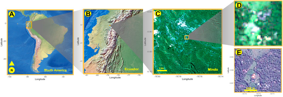
FIGURE 1. (A) Running north and south across South America, the Andes supports 15 and 12 percent of globally known plant and vertebrate species, respectively. The study area is in northern Ecuador (B), centered around a pueblo called Mindo, for which Sentinel-2 satellite rasters were cropped (C). From these rasters, we extracted tiles of 38 × 38 pixel resolution (D), with each pixel having a spatial resolution of 10 m² To manually classify individual pixels, we compared these Sentinel-derived tiles to higher resolution Airbus satellite images (E).

Huston’s Dynamic Equilibrium Hypothesis helps explain the explosion of endemic biodiversity in tropical CFs (Huston, 1979). The hypothesis proposes optimal diversity perches between environmental productivity and disturbance, between sustenance and stress.

In tropical CFs, sustenance and stress are caused by these forests’ low latitude and high altitude. At low latitudes near the equator, sustenance is spurred by year-long growth, uninterrupted by winter, and by relatively constant thermal conditions. Sustenance is further enhanced in the high altitudes of mountains by ubiquitous clouds and fog, which provide moisture for epiphytes—such as moss, lichens, bromeliads, and orchids—that have evolved the ability to draw water from the atmosphere (Gradstein et al., 2008).

But without stress in an ecosystem, only few species would dominate by outcompeting all others for resources. In tropical climates, stress is generated when high precipitation leaches minerals from the soil, lowering its fertility. Competition for nutrients prevents dominance by the few, thereby creating opportunities for the many to survive and for biodiversity to thrive.

Biodiversity is boosted further by the topographic structure of CFs. Mountains occupy a lower surface area than lowlands; they are physically separated from other mountains; and each mountain is distinct from other mountains in terms of slope, height, and lighting conditions. These topographic features create plant and animal communities that are small and isolated, where populations can diverge genetically to form endemic taxa (Myster, 2020).

Beyond biodiversity, CFs provide other ecosystem services (Figure 2). They control soil erosion and regulate water supply by intercepting, retaining, and filtering rainfall. CFs surrounding Quito, Ecuador’s capital of 1.85 million people, provide the majority of the city’s water supply (Bubb et al., 2004).

FIGURE 2

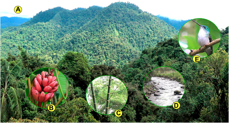
FIGURE 2. Mountainous, cloud forests (A) completely surround our study area in Mindo, Ecuador. Ecosystem services from these forests include (B) food, such as plantains; (C) building materials and carbon sequestration by Guada angustifolia, the native bamboo; (D) water; and biodiversity of epiphytes, such as orchids, and vertebrate species, such as hummingbirds (E).

Researchers concluded that contributions by CFs to carbon sequestration have been underestimated because their vegetative cover lies vertically on slopes, rather than the planar, horizontal orientation traditionally used to estimate coverage of carbon sinks (Spracklen and Righelato, 2016). In particular, Guada angustifolia, the bamboo indigenous to South America, thrives in CFs and is notably effective at converting carbon dioxide to plant matter (Muñoz-López et al., 2021). Because of its tensile strength, Guada is also used as a primary source of building materials.

Given the value of their ecosystem services, it is indeed tragic that CFs are being threatened by climate change and habitat destruction. With temperatures predicted to rise by four degrees centigrade, the cloud uplifts to which life in CFs have evolved are dissipating (Helmer et al., 2019).

Beyond climate change, other human activities are having a more direct and immediate influence on CF destruction. From 2016 to 2017, Ecuador’s Ministry of Mining increased mining concessions from 3 to 13 percent of the country’s continental land area, with the majority of this territory occurring within CFs (Roy et al., 2018).

The 2019 outbreak of the Corona virus has made this bad situation worse. The world’s unstable economy has driven up gold prices to record highs. Without jobs and money, desperate illegal miners in South America have taken advantage of pandemic lockdowns and their government’s focus on Covid-related activities to expand their activities in cloud forests (Brancalion et al., 2020).

A literature review noted recently that researchers increasingly recognize the global threats to forests, as well as the important role these forests play in creating a sustainable world. To investigate forest loss and deforestation, these researchers have been relying heavily on digital technologies—such as Remote Sensing and Artificial Intelligence (Nitoslawski et al., 2021). In this project, we based much of our investigations on these technologies.

Broadly defined, REMOTE SENSING refers to any technique obtaining information about an object without physical contact (Aggarwal, 2004). In the case of satellites, information comes in the form of fluxes in electromagnetic radiation from the remotely-sensed object to the satellite sensor.

The technology is based on two capabilities of remote-sensing satellites (Boyd, 2005). They emit electro-magnetic energy of various wavelengths; and they gather information about the distinctive manner in which an individual object reflects back the energy from each wavelength, so that its singular reflectance curves can be used to identify the object’s nature.

These capabilities have extended the scientific community’s ability to observe the world. For example, remote sensing is now being put to field-scale and site-specific agricultural use (Huang et al., 2018); to identify and classify marine debris on beaches (Acuña-Ruz et al., 2018); to assess the adequacy of environmental conditions for freshwater fisheries (Dauwalter et al., 2017); to map areas of severe soil erosion (Sepuru and Dube, 2018); and to track oil spills in the ocean (Fingas and Brown, 2018).

In 2015, the European Space Agency (ESA) launched the first of the series of Sentinel-2 satellites, which contain sensors for 13 bands of spectral wavelengths (Kaplan and Avdan 2017). Figure 3 summarizes the portion of the electromagnetic spectrum for which each band was designed, as well as the spatial resolution at which their data are collected. These bands can be classified according to their respective foci. Bands two through four extend across the red, blue, and green portions of the electromagnetic spectrum corresponding to colors perceived by humans. Bands 1, 9, and 10 have been designed to detect information for correcting distortions from atmospheric and cloud conditions. (Note that as of 2019, ESA adjusted its methods, so it no longer provides data on Band 10.) The remaining bands have been designed to collect data for specific purposes, such as detecting vegetation and moisture.

FIGURE 3

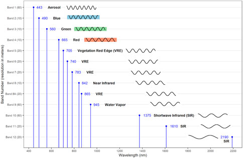
FIGURE 3. European Space Agency’s Sentinel-2 series collects information across 13 bands of the electromagnetic spectrum, sampled at four different spatial resolutions. These bands and resolution are shown on the y-axis. The x-axis shows the central wavelength value for each individual band. Bands 2–4, respectively, cover the blue, green, and red bands of light visible to humans. Bands 1, 9, and 10 are used to correct for atmospheric distortion. The remaining bands are designed for specific uses, such as detecting vegetation and moisture.

Once obtained, the values of these bands can be manipulated to compute indicators—or indices—of land use and land cover (LULC) classes. For example, one such index is the Normalized Difference Vegetation Index (NDVI) for delineating vegetative cover (Figure 4). NDVI is based on plant biology (Segarra et al., 2020). To carry out photosynthesis, green plant cells absorb solar energy in the visible light region of 400–700 μm wavelength, known as the region of photosynthetically active radiation (PAR). To avoid cellular damage, they reflect near-infrared light (NIR) wavelengths of 700–1,100 μm because NIR energy is too low to synthesize organic molecules; its absorption would merely overheat and possibly destroy plant tissue. NDVI capitalizes on this evolutionary artifact. It is the ratio of the difference between and the sum of the band values at the PAR and NIR regions. The NDVI enables researchers to translate remotely sensed band values into indicators of plant cover.

FIGURE 4

FIGURE 4. Raster indices capitalize on the fact that different objects absorb and reflect different regions of the electromagnetic spectrum. For example, green plants absorb energy in the 400–700 μm wavelengths to photosynthesize, while reflecting wavelengths of 700–1,100 μm. To serve as an indicator for vegetation, the Normalized Difference Vegetation Index calculates the ratio of the difference between and sums of Sentinel’s Bands 4 and 8.

Table 1 summarizes the raster-based indices we used in this project, along with their formulas and pertinent references. It will be useful, for later analyses, to categorize these indices by type, according to the purposes for which they were developed, such as to identify vegetation or moisture. These types are listed along Table 1, Column 3.

TABLE 1

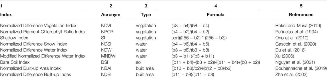
TABLE 1. These Raster Indices derive from calculations based on Sentinel-2 band values. Using the formulas in column 4, we estimated the indices in Column 1 to serve as predictors for our Random Forest models. In our project, we categorize them according to the Land Use and Land Cover type for which they were developed (column 3).

Many researchers have used these raster indices to classify LULC classes. Ma et al., for example, used three indices—the BSI, the NDVI, and the MNDWI—to model urbanization across several cities in China (Ma et al., 2019). Wasniewski et al. used the NDVI and digital elevation maps to map forest cover and forest type in Western Africa (Waśniewski et al., 2020). To develop the predictive model for their project, these latter researchers relied on Sentinel-2 images, together with the Random Forest classifier, a machine learning algorithm.

RANDOM FORESTS are called forests because they aggregate the results of many individual decision trees (Schonlau and Zou, 2020). To construct a decision tree, the analyst assumes a predictive function relates the response variable Y to the vector of predictor variables X. The decision tree algorithm maximizes the joint probability P(X,Y) by iteratively minimizing an associated loss function. In a later section, in relation to Figure 13, we discuss the graphical depiction of the algorithm’s logic.

Because the response variable Y is defined, training a decision tree risks over-fitting, a problem that sometimes besets empirical models (Pothuganti, 2018). Over-fitting occurs when the model is so dependent on the data used for training that it generates poor results when applied to other, new data. This happens because the model estimates not only the systemic relationship between predictors and the response variable, but also the random noise inherent in real-world data.

To constrain over-fitting, Breiman proposed two additional algorithms to supplement decision trees at each node (Breiman, 2001). The first randomly selects rows across the set of observations. The second randomly selects a subset of predictors in each randomly selected row.

In the Random Forest algorithm, any individual decision tree might be biased towards the particular dataset upon which it has been trained. But if analysts create a forest of thousands of such trees—with each tree modeling P(X,Y) based on randomly chosen observations—they could then pool the results from each tree in the forest, thereby reducing the influence of noisy information. To put it differently, if analysts consistently get the same model results from iteratively and randomly sampled data, then they can more confidently conclude the results are based on signals rather than noise. The algorithm’s randomizing features increase their predictive capabilities. We use this principle of randomization later, when we run simulations from an ensemble of models.

Previous studies have usefully applied Random Forests to Sentinel-2 images. For example, Ghorbanian et al. achieved accuracy rates of 85% in identifying pixels of mangrove plants (Ghorbanian et al., 2021). They report that the lowest rates of accuracy occurred in areas with mixed or boundary conditions, such as areas where mangroves tended to mix with mudflats or shallow waters. They therefore speculated that accuracy might be improved with satellite images of finer spatial scale than the 10 m² resolution of Sentinel images. In another study, the investigators applied Random Forest to Sentinel-2 images to classify LULC classes (such as cropland, water, forests, and bare soil) in Croatia, achieving an overall accuracy of 89% (Dobrinić et al., 2021). The investigators noted the usefulness of predictors such as raster indices and landscape textural features.

One other feature of Random Forest enhances its utility in this project. Because the algorithm randomly selects subsets of predictor variables at each individual tree, they are not heavily influenced by correlated predictors. That is, multicollinearity does not affect the predictive capacity of models produced by random forests, thereby enabling us to use, as predictor variables, both the computed raster indicators listed in Table 1, along with the original band values upon which they are based.

The models produced by the random forest algorithm can then be run against the predictors to generate simulations. Running random forests and generating simulations across voluminous rows and columns of data can be time-consuming. In our project, we ultimately had to analyze 1.56 × 10⁶ rows of observations with 58 columns of predictors. CLOUD TECHNOLOGY provided us with the tools we needed to analyze these data.

We received a grant from Microsoft’s Artificial Intelligence for Earth program, which provided us with a cloud platform enabling us to parallelize many of our calculations in a virtual machine with 14 CPU cores and 64 gigabytes of memory. The grant also provided us access to time-stamped and geocoded Airbus satellite rasters at 1.5 m² resolution that we used as reference images against which to compare our Sentinel images.

Cloud technology further enabled us to integrate computational efficiency with data integrity. One of our project’s objectives is to provide a low-cost method for researchers and environmental groups to apply our algorithms to monitor other vulnerable forests in the world. For this reason, we developed an R package codifying our methods. Our package, loRax, is available on the web at http://pax.green/lorax/.

We hope other researchers will use loRax to share data and metadata from their own projects. To preserve data integrity, we developed an algorithm to encode our data and metadata within blockchains. The technical foundation for bitcoins and other digital currency, the blockchain algorithm provides a way to maintain data provenance while also minimizing data tampering. Data are linked, block by block in a chain, so that each block connects to the previous one with a hash value, i.e., a randomly generated key that maps to the data in the previous block (Beck et al., 2017). The blockchain algorithm validates the series of hash values along this chain of blocks and detects any attempt to corrupt or replace the information within any block. Through this algorithm, data providers who use our R package can maintain proprietorship and provenance over their data.

Materials and Methods

Study Area

The Andes cordilleras run down Ecuador’s central spine from north to south, a narrow (150–180 km wide) stretch of mountains about 600 km long. The study area lies on the northern end of this length, on the western foothills of the volcano, Mount Pichincha. The area centers around a pueblo called Mindo, and it lies within one of the world’s five “megadiversity hotspots,” a term referring to areas containing 5 × 10³ vascular plants species per 10⁴ km².

The study area, which hereinafter we refer to as Mindo, covers 52.13 km². It has an average elevation of 1.49 kms and is bounded by the following longitudes and latitudes in the NW and SE, respectively: (−78.80, −0.04) and (−78.74, −0.1).

Data and Tools

Figure 5 provides an overview of our methods and our workflow for this project. We derived our data from three sources of satellite information: the European State Agency’s series of Sentinel-2 satellite images; the United States National Aeronautics and Space’s Administration (NASA’s) elevation data, estimated by its Global Digital Elevation Model (GDEM); and Airbus, a private aerospace company that provided us with satellite images with pixel resolution of 1.5 m². At 10 m² resolution, images from Sentinel rasters can be difficult to interpret. We therefore used the higher resolution of Airbus images to compare with the Sentinel rasters (see Figures 1D,E).

FIGURE 5

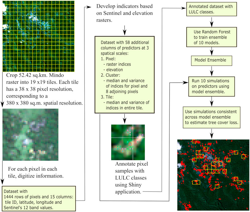
FIGURE 5. This project takes Sentinel-2 rasters as its input. From these rasters, we estimate predictors based on Sentinel’s 12 band values, as well as raster indices and elevation. To derive spatial information, we estimate the median and variance of the raster indices at three spatial scales: pixel-, cluster-, and tile-levels. We use annotated images to train an ensemble of 10 models using the Random Forest algorithm. With this model ensemble, we select pixels for which consistent simulations have been made across all 10 models. We then use these simulations to map areas of tree cover loss.

Our primary analytical tool was R, the public-domain statistical package (R Core Team, 2020). We also used SNAP, a software application developed by ESA to process, analyze, and visualize the Sentinel rasters. We codified our data, algorithms, and workflow in an R package, loRax, information about which is available at: http://pax.green/lorax/.

Select and Process Sentinel Satellite Images

We searched ESA’s data hub for satellite rasters for Mindo having the least amount of cloud cover. To minimize seasonal differences across the three time periods we downloaded, we tried choosing rasters for months that were as close to each other as possible, but this desideratum was constrained by the availability of relatively cloud-free rasters for Mindo. Listed below are the monitoring dates and filenames of the Sentinel raster we downloaded. Ultimately, to maximize our number of cloud-free pixels, we decided to compare only two time periods, 2019 and 2021. Rasters can be accessed by filename from the European Space Agency at: https://scihub.copernicus.eu/dhus/#/home.

2019-08-30 (S2B_MSIL2A_20190830T153619_N0213_R068_T17MQV_20190830T205757.SAFE)

2020-08-24 (S2B_MSIL2A_20200824T153619_N0214_R068_T17MQV_20200824T193939.SAFE)

2021-07-05 (S2A_MSIL2A_20210705T153621_N0301_R068_T17NQA_20210705T213848.SAFE)

To prepare these rasters for analysis, we used ESA’s SNAP software to resample and reproject the rasters to a 10 m² pixel resolution with the World Geodetic System (WGS84) coordinate system. We then exported the results to GeoTIFF format for further analysis with R.

Crop Raster Into Tiles

Each raster listed in above covers an area in northern Ecuador with spatial resolution of 110 × 110 kms. From each of these, we cropped rasters for our study area in Mindo. Each Mindo raster had a spatial resolution of 7.22 × 7.22 kms and pixel resolution of 722 × 722 pixels. To create even smaller rasters that were more computationally manageable, we further cropped each Mindo raster into tiles (see Figures 1C,D). Each tile has a pixel resolution of 38 × 38 pixels, corresponding to a spatial resolution of 380 × 380 m. Each Mindo raster supplies us with 361 tiles, and each tile provides us with 1,444 (38 × 38) rows of data. Ultimately, our dataset consisted of 1.56 × 10⁶ rows, i.e. (1444 pixels per tile) x (361 tiles per Mindo raster) x (3 time periods per raster). Ultimately however, to maximize the number of cloud-free pixels we could track over time, we decided to use only the rasters for 2019 and 2021.

Transform the Information in Each Tile Into a Set of Predictors

To prepare for our Random Forest model, we converted the information in the GeoTIFF of each tile into a set of predictor variables. Figure 6 summarizes our approach (The tile in Figure 6 is the same one shown in Figure 1D). All in all, we developed 58 predictors representing information for each pixel at three different spatial scales.

FIGURE 6

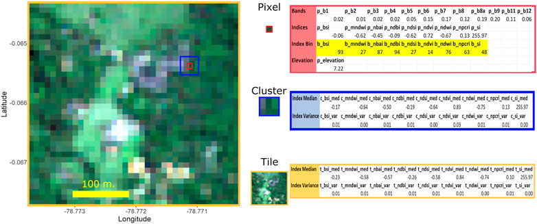
FIGURE 6. The raster above is the same one featured in Figure 1D. For each pixel (such as the one above enclosed within a red square), we developed predictors at three spatial scales: the individual pixel; the cluster of nine adjoining pixels; and all pixels within the tile. At the pixel-level, predictors consist of the 12 normalized band values; 9 raster indices; and the logarithm of the elevation level. At the cluster-level, we took the median and variance for each raster index across the nine pixels within the cluster. At the tile-level, we took the median and variance of each index across all pixels within the tile.

At the scale of individual pixels, we extracted the numeric values of each of the 12 bands recorded by the Sentinel raster and calculated the normalized values of each band. From the original, non-normalized band values, we calculated the various raster indices shown in Table 1. Lastly, we calculated the logarithm of the elevation, in meters, provided by NASA’s GDEM. To implement the annotation method we describe in the next section, we also needed to calculate the 99-percentile value within each tile for each raster index for each pixel. In the example in Figure 6, we highlight these values in yellow and refer to each as an “Index Bin.”

We hypothesized we could achieve a higher prediction accuracy if we captured spatial information about our pixel-level predictors. We therefore calculated indicators of raster index homogeneity at two other spatial scales. At a cluster level—for each pixel and its eight adjoining pixels—we calculated the median and variance of each raster index. At the tile level, we performed the same calculations for median and variance of each raster index across all pixels in the tile.

In Figure 6 and in the rest of the paper, we use the following the notation to refer to predictors. We use the prefix “p”, “c”, and “t” to refer to the scale (pixel, cluster, and tile) of the predictor. This is followed by the acronym for each index (e.g., NDVI, BSI, SI, etc.) as denoted in Table 1. For the cluster- and tile-level predictors, we use the suffix “med” or “var” to refer to whether the predictor represents the median or variance of the group of pixels. So, for example, the notation “t_ndvi_med” refers to the NDVI’s median value across all pixels in a tile.

Annotate Tile Samples With Land Use and Land Cover Classes

Before training our model, we first needed to annotate samples from our data. To perform our annotations, we developed an interactive application using R’s Shiny package. An interactive demonstration of the Shiny app is available at http://pax.green/lorax/. The application is summarized in Figure 7 (The raster in Figure 7A is the upper-right cross-section of the raster from Figure 6. The pixel within the red square is the same pixel featured in Figure 6).

FIGURE 7

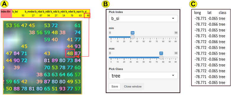
FIGURE 7. The raster above (A) is the upper-right cross-section of the raster featured in Figure 6, with a red square around the same pixel from Figure 6. Within each tile, for each raster index for each pixel, we took the 99% percentile value of the index, which we refer to as the Index Bin. For example, the selected pixel had an SI (shadow index, used to monitor tree canopy) value of 255.97 (see Figure 6). The pixel has an SI Index Bin (b_si) value of 48. To annotate or tag a pixel, we developed a Shiny, interactive application (B) for our R package, loRax. In the example above, we selected “b_si” from the drop-down box and manipulated the scroll bars to select minimum/maximum values of 33/77. Colored numbers corresponding to the Index Bin values of each pixel within this range appeared on the raster image (A). After comparing the resulting image with the higher resolution Airbus image (see Figures 1D,E), we selected the class “tree” from another drop-down list (B) to save the class and location of the selected pixels to file (C).

As we stated earlier, for each raster index for each tile, we categorized each pixel value into 0-99 percentiles, which we refer to as an Index Bin. For example, in Figure 7A, the selected pixel’s value for the Shadow Index (si)—a raster index used to estimate tree canopy cover—falls into the 48th percentile, or Index Bin.

Using loRax’s Shiny application, we selected “b_si” (for binned Shadow Index) from the drop-down list that allows one to choose from any of the indices listed in Table 1 (see Figure 7B). We then manipulated scroll bars to choose 33 and 77 as the minimum and maximum values, respectively, for the selected tile’s Index Bins for SI. On the tile’s satellite image (Figure 7A), pixels with Index Bin values between and including these min/max numbers interactively appeared as colored numbers (their Index Bin values). We then compared this image to the higher resolution image from Airbus (see Figures 1D,E), as well as Figures 9A,C). Once we were satisfied that the colored pixels corresponded to the corresponding LULC class (in this example, tree cover), loRax enabled us to select the LULC class from another drop-down list (Figure 7B) and to save the results—i.e. the pixels’ LULC class, along with their location (Figure 7C)—to a file for inclusion in the dataset for annotated LULC classes.

Train the Random Forest Models and Run Simulations

These annotated LULC classes served as the response variables for the Random Forest algorithm, and the 58 variables shown in Figure 6 served as predictors. Before running the algorithm, we split the data into two bins—one for training and another for testing the model. Table 2 summarizes the number of annotated pixels within each class. In total, we had 265,566 pixels in our annotated dataset, with six classes: tree, grass, water, soil, built, and cloud. Water had the fewest annotations, with 6,132 pixels. For each iteration of training our Random Forest model, we took 70 and 30 percent of 6,132 as the number of pixels within each class to respectively train and test the model. Because we had sufficient annotations for the other classes, we over-sampled from these classes, as detailed in Table 2.

TABLE 2

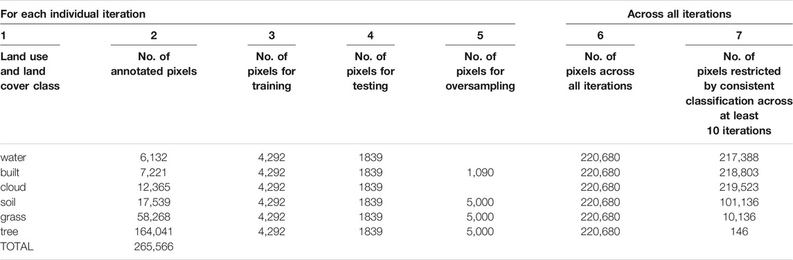
TABLE 2. We developed a Model Ensemble based on 120 iterations of the Random Forest algorithm on our annotated dataset. We sampled and manually classified 2.65 × 10⁵ pixels. For each iteration, pixel numbers for training, testing, and oversampling are listed in columns 3 through 5. To evaluate the accuracy of our model ensemble, we developed Confusion Matrices for two types of test data. In column 6, we combined all test results across all iterations. In column 7, we selected only those pixels that were classified consistently across at least 10 iterations.

To create an ensemble of models, we ran Random Forest 120 times, with each iteration’s model based on randomly sampled data. The testing data thus produced were of two types. For the first type, we merged the test data from across the 120 iterations, generating 220,680 (120 iterations x 1839 rows of test data per iteration) as shown in Table 2’s Column 6. For the second type, we created a second test dataset, one that was restricted by two criteria: 1) the pixel needed to have been simulated by at least 10 iterations; and 2) the classification of the pixel must have been consistent across all 10 iterations (Table 2’s Column 7).

For this second, “restricted” dataset, trees had fewer data (146) because it was a class with many annotated pixels (164,041). Each pixel therefore had a low probability of being randomly selected over 120 iterations, making it difficult for this class to fulfill the first criteria of needing to have been simulated for at least 10 iterations.

R’s Random Forest package computes the Mean Decrease Accuracy (MDA), a measure of each predictor’s influence on model accuracy. After an initial run of the Random Forest using all predictors, we selected those predictors with an MDA value of at least 0.02. Our objective was to choose predictors that were influential, but not to have so many predictors that the models would run the risk of over-fitting.

After running the Random Forest, we applied Principal Component Analysis to our annotated dataset to better understand the influence of each predictor on each LULC class (Jolliffe and Cadima, 2016).

Results

Assess Simulation Accuracy With Confusion Matrix

To evaluate accuracy across the simulations from our ensemble of 10 models, we developed the Confusion Matrices shown in Figure 8. Figure 8A’s Confusion Matrix is based on test data of the first type, which merged all test data across the 120 iterations. In this matrix, the models simulated tree cover correctly 96.72% of the time; they misidentified tree cover as grass 2.08% of the time (for clarity, only error rates greater than or equal to 1 percent are shown).

FIGURE 8

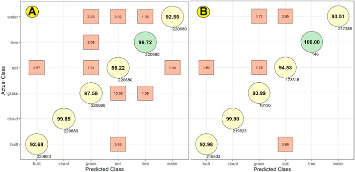
FIGURE 8. These Confusion Matrices are based on results from Random Forest tests for two different types of data (see Table 2). In (A), we estimated accuracy scores based on all the test data derived from the 120 iterations we ran of Random Forest. In (B), we selected pixels that were classified consistently across at least 10 iterations.

The highest rates of error of the Random Forest simulations occurred in the models’ simulation of grass cover. These grass simulations generated a true positive accuracy rate of 87.58%. For grass, the models generated false positives 11.62% of the time, classifying as grass those pixels that were actually soil (7.31%), tree cover (2.08%), and water (2.23%). The models also generated false negatives for grass, misclassifying as soil (10.56%) and tree (1.09%) pixels that should have been classified as grass.

Assess Simulation Accuracy With Satellite Images and Field Visits

We tried evaluating simulation accuracy by comparing our simulations against the higher resolution Airbus satellite images. But because of the temporal mismatch between the Sentinel and Airbus rasters, this approach can lead to misleading results. Figure 9 provides an example of the problems of temporal mismatch.

FIGURE 9

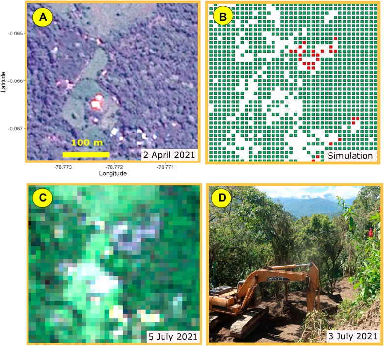
FIGURE 9. (A) Airbus mid-resolution image of a Mindo tile for which (B) the model simulation showed tree cover loss in the tile. The Airbus image (taken on April 2021) does not show tree cover loss. But the model was based on a Sentinel raster (C) taken on July 2021. A site visit clarified the discrepancy. Construction of a new subdivision broke ground (D) after the Airbus image was taken in April. Sentinel’s July image and the Random Forest model detected the more recent pattern of tree cover loss.

To calculate loss of tree cover, we filtered our data in two steps. First, we selected only those pixels in Mindo that were cloud-free across two time periods (2019 and 2021). Second, we used only the “restricted” test data. For these data, we defined a pixel as having lost tree cover if the pixel was classified as tree cover in 2019 but was classified as some other class in 2021.

We also identified tiles having a relatively higher proportion of tree cover loss—at least 5%. We refer to these tiles as “tree loss hotspots.” To avoid the bias of small samples, we selected only those tiles that retained at least 1,000 pixels after filtering for cloud cover. We then calculated the proportion within these tiles of pixels identified as having lost tree cover.

Given the Covid lock-down, we could only visit “tree loss hotspots” within walking distance of Mindo’s central plaza. Fortunately, within one such area, we obtained results enabling us to verify our simulations.

In Figure 9B, the model simulation for 2021 indicates loss of tree cover (shown as red pixels) that do not appear in the corresponding Airbus image (Figure 9A). A visit to the site clarified the reasons for this apparent discrepancy. The Airbus image was taken in April, while the simulation was derived from the Sentinel raster for July (Figure 9C). A site visit enabled us to confirm that new construction had broken ground between April and July (Figure 9D).

Evaluate Influence of Predictor Variables With Mean Decrease in Accuracy

Figure 10 shows the relative importance of the various predictors, based on the mean decrease in accuracy (MDA). This metric estimates relative importance by calculating how removing a predictor affects prediction accuracy. As discussed in Figure 4 and its accompanying text, each predictor can be characterized by type (i.e., by the purpose for which each index was developed, such as to identify vegetation or moisture); scale (pixel-, cluster-, or tile-levels); and, at the cluster- and tile-level, by measures of homogeneity (median and variance). Figure 10’s coloration of points characterizes each predictor by scale. As shown in the figure’s inset, the most influential predictors, as measured by MDA, are a mix of predictors varying by type, scale, and measure of homogeneity.

FIGURE 10

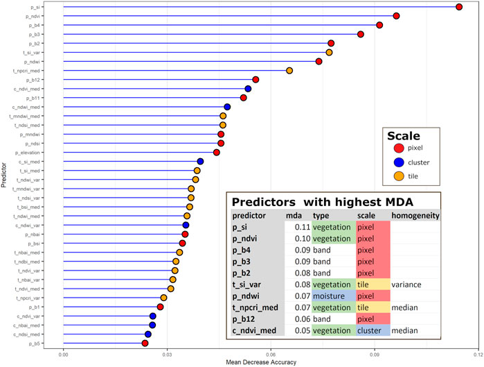
FIGURE 10. Mean Decrease Accuarcy measures each predictor’s influence on the LULC classes simulated by the Random Forest Model. Each predictor has three attributes: type, scale, and homogeneity. Type refers to how they are used (e.g., to detect vegetation, water, etc.). Scale is the spatial level at which each was measured. Homogeneity is the median or variance of each raster index at the cluster or tile levels. The most influential predictors are shown inset. They are a mix of predictors varying by type, scale and homogeneity.

Evaluate Influence of Predictor Variables With Principal Component Analysis

Principal Component Analysis (PCA) simplifies high-dimensional, complex data by extracting features of the data and then projecting these features on to lower dimensions (called principal components). These features are extracted and projected one dimension at a time; each dimension cumulatively explains the variability of data features, and each succeeding dimension is estimated independently from preceding dimensions.

We conducted a PCA on the annotated dataset used to train and test our Random Forest model. The first three dimensions, results for which are summarized in Figure 11’s biplots, explain 70% of the variability across our dataset. The density of points for each class across the PCA quadrants is shown as color gradients on the biplots, with diamond points indicating each class’s center of highest density.

FIGURE 11

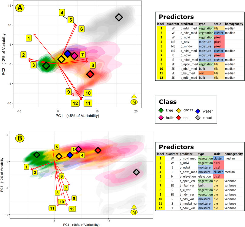
FIGURE 11. We conducted a PCA on our annotated dataset. The first three dimensions (PC1, PC2, and PC3) explain 70% of the data variability. Individual PCA scores are shown above as differently colored density clouds, with the highest density points for each class shown as diamonds. The Random Forest’s high accuracy scores for cloud and tree conform to the observation that their PCA scores cluster distinctly at the east and west quadrants of the PCA. Contrariwise, the individual scores for the other classes merge closely together near the point of origin. PC1’s west and east quadrants are dominated by loadings related to vegetation and moisture, respectively. Both PC2’s and PC3’s southern quadrant is dominated by tile-level measures of homogeneity—median and variance for PC2 and PC3, respectively.

The influence of a predictor along one dimension is measured by its so-called loading, represented on the biplot as the length of each arrow. The angles between arrows show the correlation between predictors. For example, in Figure 11A, along the PCA’s first dimension, points 2 and 3 (c_ndvi_med and p_ndvi, the cluster-level median and pixel-level values of NDVI) are closely related. Points 7 and 8 (p_ndwi and c_ndwi_med, the pixel-level and cluster-level median values for NDWI) are closely related; however, compared to points 2 and 3, they exert an opposite influence on the first dimension. On the other hand, along the second dimension, point 12 lies on the PCA’s southern quadrant. This point, representing t_ndbi_med, exerts an influence that is orthogonal to any of the points along the first dimension.

Map of Tree Loss

One of our primary objectives was to produce a map of individual pixels of tree loss and of tiles that are “tree loss hotspots.” We have shared this map, shown in Figure 12 with environmentally-motivated stakeholders in Mindo to help them focus their efforts on these areas of greatest concern.

FIGURE 12

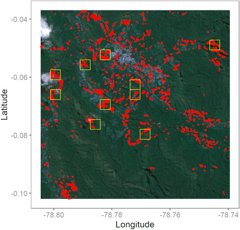
FIGURE 12. Individual red dots show areas of tree cover loss in Mindo. Yellow boxes indicate tiles where tree cover loss equaled or exceeded 5% of the tile area. Based on our model results, the total area of tree cover loss between August 2019 and July 2021 is 0.61 km²—1.17% of the study area.

Discussion

The convergence of remote sensing, Artificial Intelligence, and cloud computing supplied us with massive amounts of data and with the computing power to process them. We set out to develop a workflow for monitoring deforestation with satellite data and to build a corresponding R package that is scalable and transferrable for use by others to protect forests across the globe. For our tool, loRax, to be credibly implemented, it must deliver results that are accurate, in a way that is relatively transparent.

Artificial Intelligence has been criticized as being a “black box” through which one feeds copious data to be digested by obtuse algorithms, and from which predictive simulations are regurgitated (Castelvecchi, 2016). Although the mathematical computations of the Random Forest can be obtuse, we have tried in this paper to provide an intuitive explanation of its theoretical underpinnings, which we believe can be communicated more easily than those of, say, a Convolutional Neural Network (CNN) (LeCun et al., 2015). Additionally, most pre-trained CNNs have been built on RGB images (Senecal et al., 2019). In the future, researchers may yet develop CNNs that can analyze more than three bands and that would not require the computational resources typically demanded by deep CNNs.

For the present, we hypothesized we could use Random Forest to obtain useful information from the 12 bands of Sentinel rasters. We further hypothesized that we could improve the accuracy of our simulations:

by developing predictors to capture spatial information; and

by generating these simulations with a model ensemble.

Figure 8B’s Confusion Matrix suggests there is much analytical value to be gained from these two innovations.

Influence of Individual Predictors on Simulated Classes

As an additional step towards model transparency, we also investigated how the predictors might be influencing model simulations. Figure 10’s MDA indicates that the predictors wielding the most influence are a combination of normalized band values; raster indices for vegetation and moisture; and measures of homogeneity of these indices across spatial scales. Out of the 38 predictors used for the Random Forest, 15 were at the pixel level and another 16 at the tile level—9 for the median and seven for the variance. This result confirms the importance of information provided by our predictors of spatial homogeneity. Out of all predictors, 13 were for vegetation-related indices and 12 for moisture-related indices.

Figure 11’s PCAs provide additional insight about the predictors. While Random Forests maximize the joint probability between predictor and response variables, PCAs aim to group predictors into fewer dimensions by eliminating information redundancies in the data. In doing so, the PCA provides insight on how individual predictors might be influencing the Random Forest simulations.

The PCAs indicate 70% of variability in the dataset could be accounted for in the PCA’s first three dimensions: respectively 48, 12, and 10 per cent in the first, second, and third dimensions. The first dimension is defined by raster indices for vegetation and moisture lying west and east, respectively, of the point of origin (POI). In the second and third dimensions, predictors south of the POI relate to spatial information at the tile level—the tile median in the second dimension and the tile variance in the third. These results conform to Figure 10’s MDA indicating the importance of spatial information to complement water- and vegetation-related raster indices at the individual pixel level.

Looking beyond the PCA loadings to the scores for individual observations, we observe that these PCA scores are consistent with Figure 8’s Confusion Matrices. Figure 8 shows simulations for tree and cloud cover to be highly accurate (more than 99%). In Figure 11’s PCA, individual scores for tree and clouds form distinct clusters lying west and east on the PCA quadrants. Contrariwise, data for grass, soil, water, and built classes are widely dispersed around the POI. Although the highest density points for these classes are distinct, their individual points merge with one another across the four quadrants of the PCA. This might account for their relatively lower accuracies in Figure 8’s Confusion Matrices. We hypothesize that the electromagnetic, spectral signals sent by objects in the grass, soil, water, and built LULC classes are less distinctive than those sent by the tree- and cloud-cover classes.

At this juncture, one point merits mention. This paper’s senior author has co-written several policy- and law-oriented papers on the importance of understanding a model’s epistemic framework, i.e., its assumptions and underlying theoretical foundations (Fisher et al., 2014). PCA and Random Forest are built upon different epistemic foundations. That each corroborates the other’s results should provide one with a measure of confidence in the models’ simulations.

Visualizing the Random Forest

With a better understanding of the influence of individual predictors on the modeling process, with a mind to enhance the transparency of our modeling process, we now visualize the logic of the Random Forest algorithm. To do so, we trained a model using a highly simplified annotated dataset which we created by modifying the original annotated dataset as follows:

We subset the response variables to only two classes—tree and grass.

We subset the predictors to only three—p_ndwi, p_ndwi, and t_mndwi_var.

We binned the raw predictor values into three percentile groups.

We ran the Random Forest on this simplified annotated dataset to produce a model distinguishing between grass and tree cover. Figure 13 graphically depicts the logic through which the algorithm produced a single decision tree. The decision tree goes through a series of Yes/No choices based on the value of each predictor, with each tree branch leading to either “grass” or “tree.” During the training period with our full, annotated dataset, Random Forest aggregates the results of thousands of such trees to generate the set of rules the models use to classify the different LULC classes.

FIGURE 13

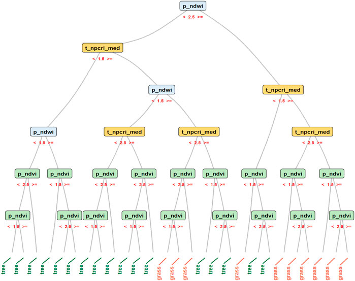
FIGURE 13. This graphic visualizes the Random Forest Algorithm’s logic for a single Decision Tree for a simplified annotated dataset. The original dataset was filtered for data with the LULC classes of “tree” and “grass;” only three predictors were selected; and values of the predictors were grouped into three percentile bins. In this example, rules govern whether a branch in the Decision Tree ultimately leads to a pixel being classified as “grass.” Generally, (A) p_ndwi must be≥2.5; and (B) t_npcri_med must be≥1.5. If (A) is true and (B) is false, then p_ndvi must be <1.5. If (A) and (B) are false, then p_ndwi must be >1.5 and p_ndvi must be <2.5. Simulations from our ensemble of Random Forest models are the net, probabilistic result from thousands of such trees for all predictors and response variables in our annotated dataset.

We glean a plausible narrative from Figure 13’s decision tree and Figure 11’s PCAs. Although NDVI and NPCRI have both been developed to detect vegetation, Figure 13 suggests higher NPCRI values are associated with grass cover. Figure 11B’s PCA suggests that the tile-level variance of NPCRI exerts an influence on the third dimension that is opposite that of elevation. These results suggest a spatial structure consistent with Mindo’s settlement pattern. Tree cover tends to prevail at higher elevations. At lower elevations, in Mindo’s valleys, there is greater variability in the distribution of trees and pastureland.

Addressing Model Uncertainties

Uncertainties are inherent in the modeling process (Wagner et al., 2010). As highlighted in Figure 9, a significant source of uncertainty stems from the temporal mismatch between the Sentinel rasters and whichever high-resolution image one uses to verify the simulations. To put it another way, “model errors” may have as much to do with the manual annotations of the training data as it does with the algorithms of Artificial Intelligence.

To constrain the latter type of error, we attempted to deal with its uncertainties in three ways. First, for those LULC classes for which we had sufficient data—soil, tree, and grass—we oversampled for the training set for the Random Forest.

Second, we ran simulations based on an ensemble of models. Each iteration of the Random Forest algorithm was based on randomly sampled data from the annotated dataset. In our earlier discussion on the theory of Random Forests, we noted that if analysts consistently get the same model results from iteratively and randomly sampled data, they can more confidently conclude the results are based on signals rather than noise. We extended this principle to ensemble modeling, and Figure 8B’s Confusion Matrix shows promising results.

Third, to identify those areas with tree loss between 2019 and 2021, we selected only those pixels which were classified consistently across all simulations from an ensemble of at least 10 model iterations.

Given these precautions and given that we filtered out pixels that were cloud-covered, we suggest that if anything, our results likely underestimate forest loss in Mindo. We were hampered by our inability to find more cloud-free satellite rasters for Mindo than we would have wanted for our analyses. We suspect this would not have been the case for areas thought to offer more commercial opportunities than Mindo, where ecosystem services redounding to global sustainability go largely unpriced by the market.

Topics for Future Research

There is considerable future work to be done. First, it is generally recognized that data-intensive, place-based models may have limited application beyond the region from which data were collected. Figure 11’s PCAs are consistent with Mindo’s spatial structure. In Mindo, people have tended to settle in valleys at lower elevations, where the landscape is crisscrossed by rivers, pastures, and homes. This would account for the importance of spatial measures of homogeneity along dimensions 2 and 3, particularly in dimension 3’s measures of variance, which have an inverse relationship with elevation. It would be fruitful to investigate how our models would compare to models run in areas with vastly different settlement patterns.

Second, at the code level, we have tried to speed our computations by using parallel-processing whenever possible. We also have tried to use transparent data structures by organizing our data hierarchically and grouping pixels within tiles. We hope that other data scientists can improve the efficiency of our workflow while maintaining clarity and transparency in their algorithms and data structures.

Third, we cropped the Mindo raster into 380 × 380 m tiles because this resolution roughly corresponded to the spatial resolution of Google’s satellite images at Google Map’s API’s 16x resolution. (We did this before being notified we received a grant to purchase Airbus images.) It would be worth exploring whether a different spatial resolution for tiles would generate more accurate results.

Fourth, to generate spatial information, our current algorithms estimate tile- and cluster-level median and variance. We can improve upon these algorithms by clustering pixels within each tile into segments where pixels share similar attributes. The shape and area of the segments might serve as predictors that would provide greater accuracy to our predictions.

Fifth, we are presently trying to classify LULC classes and predictors across the Mindo tiles into some typology of tiles. We then intend to integrate this typology of tiles with bird observations. In Mindo, in a roughly 100-hectare area of forest reserve, 356 species of birds have been identified (Stevens et al., 2021). Our objective is to build a hierarchical, Bayesian model relating Mindo’s land attributes with bird counts obtained from Cornell’s ebird database (Wood et al., 2011).

Finally, a fruitful ground for social science research is how to use computational models for forest governance. Elinor Ostrom’s work on how communities collectively manage shared resources emphasizes the importance of performance measures (Anderies et al., 2013). It would be extremely useful to explore how deforestation models based on public data and Artificial Intelligence can be communicated more clearly and credibly to community stakeholders. As a corollary, it would be worth investigating whether model results can be used as performance measures to encourage community-based tree conservation activities.

Conclusion

To summarize our project in concrete terms, we are accessing data from observations made from a distance of 786 km. (Sentinel’s orbiting altitude) to make predictions about whether or not an area half the size of a singles tennis court (roughly the spatial resolution of an individual pixel from Sentinel) is covered by trees. Despite this task’s challenges, Figure 8’s Confusion Matrices indicate a probability of more than 96% that our simulations of tree cover loss would be correct. To summarize Figure 12’s results in concrete terms, in our study area of 52 km² (about a third the size of Washington, DC), tree cover loss over the past 2 years added up to an area of 0.61 km², about the size of 3,106 tennis courts.

We had set out to extract the signals in our satellite images and to transform them into actionable information based on evidence. For this reason, we exercise conservatism in our modeling approach, as described in the previous section. For the same reason, we developed our R package, loRax, and based it primarily on open-access data. It is the reason our package uses blockchain technology to preserve the integrity and provenance of the annotated dataset.

Briefly put, we hope both our algorithms and data will be used by researchers, environmental groups, and governmental agencies to protect forests across the globe. We hope the results generated by anyone using loRax can serve as presumptive evidence that an area is losing forest cover, particularly in those countries that are resource-poor and that need to prioritize areas for conservation or for other forms of intervention. We hope that others who use the R package will block-chain and share their annotated data (or improve upon our algorithms) so that collectively, we can increase the accuracy, and therefore the defensibility, of its simulations of tree cover loss, thereby boosting our ability to conserve this precious resource.

Data Availability Statement

The datasets presented in this study can be found in online repositories. The names of the repository/repositories and accession number(s) can be found below: http://pax.green/lorax/.

Author Contributions

PP conceived of the project, wrote the code, developed the methodology, obtained the data, and conducted the literature review. CP annotated several of the tiles used to train the Random Forest model. They also clarified the over-all concept and methodology with the senior author.

Funding

Microsoft’s AI for Earth program provided free access to their Azure cloud platform. The program also arranged for free access to Airbus satellite rasters. This project was supported by the community of Mindo. The pueblo’s people sustained the work by offering hospitality and by providing us with the oral history of the area. This helped inform our understanding of Mindo’s spatial structure.

Conflict of Interest

The authors declare that the research was conducted in the absence of any commercial or financial relationships that could be construed as a potential conflict of interest.

Publisher’s Note

All claims expressed in this article are solely those of the authors and do not necessarily represent those of their affiliated organizations, or those of the publisher, the editors and the reviewers. Any product that may be evaluated in this article, or claim that may be made by its manufacturer, is not guaranteed or endorsed by the publisher.

References

Acuña-Ruz, T., Uribe, D., Taylor, R., Amézquita, L., Guzmán, M. C., Merrill, J., et al. (2018). Anthropogenic marine Debris over Beaches: Spectral Characterization for Remote Sensing Applications. J. Remote Sensing Environ. 217, 309–322. doi:10.1016/j.rse.2018.08.008

CrossRef Full Text | Google Scholar

Aggarwal, S. (2004). Principles of Remote Sensing. Geneva, Switzerland: World Meteorological Oganisation.

Google Scholar

Anderies, J. M., Folke, C., Walker, B., and Ostrom, E. (2013). Aligning Key Concepts for Global Change Policy: Robustness, Resilience, and Sustainability. J. Ecol. Soc. 18 (2), 8. doi:10.5751/es-05178-180208

CrossRef Full Text | Google Scholar

Beck, R., Avital, M., Rossi, M., and Thatcher, J. B. (2017). Blockchain Technology in Business and Information Systems Research. Wiesbaden, Germany: Springer.

Google Scholar

Bouhennache, R., Bouden, T., Taleb-Ahmed, A., and Cheddad, A. (2019). A New Spectral index for the Extraction of Built-Up Land Features from Landsat 8 Satellite Imagery. Geocarto Int. 34 (14), 1531–1551. doi:10.1080/10106049.2018.1497094

CrossRef Full Text | Google Scholar

Boyd, D. (2005). Physical Basis of Remote Sensing. J. J. Geoinformatics 1, 67–81.

Google Scholar

Brancalion, P. H. S., Broadbent, E. N., de-Miguel, S., Cardil, A., Rosa, M. R., Almeida, C. T., et al. (2020). Emerging Threats Linking Tropical Deforestation and the COVID-19 Pandemic. J. Perspect. Ecol. conservation Biol. 18 (4), 243–246. doi:10.1016/j.pecon.2020.09.006

CrossRef Full Text | Google Scholar

Breiman, L. (2001). Random Forests. J. Machine Learning 45 (1), 5–32. doi:10.1023/a:1010933404324

CrossRef Full Text | Google Scholar

Bruijnzeel, L., Kappelle, M., Mulligan, M., and Scatena, F. (2010). Tropical Montane Cloud Forests: State of Knowledge and Sustainability Perspectives in a Changing World. Cambridge, United Kingdom: Cambridge University Press.

Google Scholar

Bubb, P., May, I. A., Miles, L., and Sayer, J. (2004). Cloud forest Agenda. Cambridge, United Kingdom: UNEP-WCMC biodiversity series.

Google Scholar

Castelvecchi, D. (2016). Can We Open the Black Box of AI? Nature 538 (7623), 20–23. doi:10.1038/538020a

PubMed Abstract | CrossRef Full Text | Google Scholar

Clark, L. G., and Mason, J. J. (2019). Redescription of Chusquea Perligulata (Poaceae: Bambusoideae: Bambuseae: Chusqueinae) and Description of a Similar but New Species of Chusquea from Ecuador. Phytotaxa 400 (4), 227–236. doi:10.11646/phytotaxa.400.4.2

CrossRef Full Text | Google Scholar

Dauwalter, D. C., Fesenmyer, K. A., Bjork, R., Leasure, D. R., and Wenger, S. J. (2017). Satellite and Airborne Remote Sensing Applications for Freshwater Fisheries. Fisheries 42 (10), 526–537. doi:10.1080/03632415.2017.1357911

CrossRef Full Text | Google Scholar

Dobrinić, D., Gašparović, M., and Medak, D. (2021). Sentinel-1 and 2 Time-Series for Vegetation Mapping Using Random Forest Classification: A Case Study of Northern Croatia. Remote Sensing 13 (12), 2321. doi:10.3390/rs13122321

CrossRef Full Text | Google Scholar

Du, Y., Zhang, Y., Ling, F., Wang, Q., Li, W., and Li, X. (2016). Water Bodies' Mapping from Sentinel-2 Imagery with Modified Normalized Difference Water Index at 10-m Spatial Resolution Produced by Sharpening the SWIR Band. Remote Sensing 8 (4), 354. doi:10.3390/rs8040354

CrossRef Full Text | Google Scholar

Fingas, M., and Brown, C. E. (2018). A Review of Oil Spill Remote Sensing. Sensors 18 (1), 91. doi:10.3390/s18010091

PubMed Abstract | CrossRef Full Text | Google Scholar

Fisher, E., Pascual, P., and Wagner, W. (2014). Rethinking Judicial Review of Expert Agencies. Tex. L. Rev. 93, 1681.

Google Scholar

Foster, P. (2001). The Potential Negative Impacts of Global Climate Change on Tropical Montane Cloud Forests. Earth-Science Rev. 55 (1-2), 73–106. doi:10.1016/s0012-8252(01)00056-3

CrossRef Full Text | Google Scholar

Gascoin, S., Barrou Dumont, Z., Deschamps-Berger, C., Marti, F., Salgues, G., López-Moreno, J. I., et al. (2020). Estimating Fractional Snow Cover in Open Terrain from sentinel-2 Using the Normalized Difference Snow index. Remote Sensing 12 (18), 2904. doi:10.3390/rs12182904

CrossRef Full Text | Google Scholar

Ghorbanian, A., Zaghian, S., Asiyabi, R. M., Amani, M., Mohammadzadeh, A., and Jamali, S. (2021). Mangrove Ecosystem Mapping Using Sentinel-1 and Sentinel-2 Satellite Images and Random forest Algorithm in Google Earth Engine. Remote Sensing 13 (13), 2565. doi:10.3390/rs13132565

CrossRef Full Text | Google Scholar

Gradstein, S. R., Homeier, J., and Gansert, D. (2008). The Tropical Mountain forest; Patterns and Processes in a Biodiversity Hotspot. Göttingen, Germany: Universitätsverlag Göttingen.

Google Scholar

Guayasamin, J. M., Cisneros-Heredia, D. F., Vieira, J., Kohn, S., Gavilanes, G., Lynch, R. L., et al. (2019). A New Glassfrog (Centrolenidae) from the Chocó-Andean Río Manduriacu Reserve, Ecuador, Endangered by Mining. PeerJ 7, e6400. doi:10.7717/peerj.6400

PubMed Abstract | CrossRef Full Text | Google Scholar

Helmer, E. H., Gerson, E. A., Baggett, L. S., Bird, B. J., Ruzycki, T. S., and Voggesser, S. M. (2019). Neotropical Cloud Forests and Páramo to Contract and Dry from Declines in Cloud Immersion and Frost. PloS one 14 (4), e0213155. doi:10.1371/journal.pone.0213155

PubMed Abstract | CrossRef Full Text | Google Scholar

Huang, Y., Chen, Z.-x., Yu, T., Huang, X.-z., and Gu, X.-f. (2018). Agricultural Remote Sensing Big Data: Management and Applications. J. Integr. Agric. 17 (9), 1915–1931. doi:10.1016/s2095-3119(17)61859-8

CrossRef Full Text | Google Scholar

Huston, M. (1979). A General Hypothesis of Species Diversity. The Am. Naturalist 113 (1), 81–101. doi:10.1086/283366

CrossRef Full Text | Google Scholar

Jolliffe, I. T., and Cadima, J. (2016). Principal Component Analysis: a Review and Recent Developments. Phil. Trans. R. Soc. A. 374 (2065), 20150202. doi:10.1098/rsta.2015.0202

PubMed Abstract | CrossRef Full Text | Google Scholar

Kaplan, G., and Avdan, U. (2017). Mapping and Monitoring Wetlands Using Sentinel-2 Satellite Imagery. ISPRS Ann. Photogramm. Remote Sens. Spat. Inf. Sci. IV-4/W4, 271–277. doi:10.5194/isprs-annals-iv-4-w4-271-2017

CrossRef Full Text | Google Scholar

LeCun, Y., Bengio, Y., and Hinton, G. (2015). Deep Learning. Nature 521 (7553), 436–444. doi:10.1038/nature14539

PubMed Abstract | CrossRef Full Text | Google Scholar

Ma, X., Li, C., Tong, X., and Liu, S. (2019). A New Fusion Approach for Extracting Urban Built-Up Areas from Multisource Remotely Sensed Data. Remote Sensing 11 (21), 2516. doi:10.3390/rs11212516

CrossRef Full Text | Google Scholar

Muñoz-López, J., Camargo-García, J. C., and Romero-Ladino, C. (2021). Valuation of Ecosystem Services of Guadua Bamboo (Guadua Angustifolia) forest in the Southwestern of Pereira, Colombia. Caldasia 43 (1), 186–196. doi:10.15446/caldasia.v43n1.63297

CrossRef Full Text | Google Scholar

Myster, R. W. (2020). Disturbance and Response in the Andean Cloud forest: A Conceptual Review. Bot. Rev. 86 (2), 119–135. doi:10.1007/s12229-020-09219-x

CrossRef Full Text | Google Scholar

Nguyen, C. T., Chidthaisong, A., Kieu Diem, P., and Huo, L.-Z. (2021). A Modified Bare Soil Index to Identify Bare Land Features during Agricultural Fallow-Period in Southeast Asia Using Landsat 8. Land 10 (3), 231. doi:10.3390/land10030231

CrossRef Full Text | Google Scholar

Nitoslawski, S. A., Wong‐Stevens, K., Steenberg, J. W. N., Witherspoon, K., Nesbitt, L., and Konijnendijk van den Bosch, C. C. (2021). The Digital Forest: Mapping a Decade of Knowledge on Technological Applications for forest Ecosystems. Earth's Future 9 (8), e2021EF002123. doi:10.1029/2021ef002123

CrossRef Full Text | Google Scholar

Olson, D. M., and Dinerstein, E. (2002). The Global 200: Priority Ecoregions for Global Conservation. Ann. Mo. Bot. garden 89, 199–224. doi:10.2307/3298564

CrossRef Full Text | Google Scholar

Ono, A., Kajiwara, K., and Honda, Y. (2010). Development of New Vegetation Indexes, Shadow index (SI) and Water Stress Trend (WST). Intern. Arch. Photogrammetry, Remote Sensing Spat. Inf. Sci. 38, 710–714.

Google Scholar

Peñuelas, J., Gamon, J. A., Fredeen, A. L., Merino, J., and Field, C. B. (1994). Reflectance Indices Associated with Physiological Changes in Nitrogen-And Water-Limited sunflower Leaves. Remote sensing Environ. 48 (2), 135–146.

Google Scholar

Pothuganti, S. (2018). Review on Over-fitting and Under-fitting Problems in Machine Learning and Solutions. Int. J. Adv. Res. Electr. Electron. Instrumentation Eng. 7 (9), 3692–3695. doi:10.15662/IJAREEIE.2018.070901

CrossRef Full Text | Google Scholar

R Core Team (2020). R: A Language and Environment for Statistical Computing. Vienna, Austria: R Foundation for Statistical Computing.

Google Scholar

Reyes-Puig, C., Wake, D. B., Kotharambath, R., Streicher, J. W., Koch, C., Cisneros-Heredia, D. F., et al. (2020). Two Extremely Rare New Species of Fossorial Salamanders of the Genus Oedipina (Plethodontidae) from Northwestern Ecuador. PeerJ 8, e9934. doi:10.7717/peerj.9934

PubMed Abstract | CrossRef Full Text | Google Scholar

Rokni, K., and Musa, T. A. (2019). Normalized Difference Vegetation Change index: A Technique for Detecting Vegetation Changes Using Landsat Imagery. Catena 178, 59–63. doi:10.1016/j.catena.2019.03.007

CrossRef Full Text | Google Scholar

Romero, B. J. Z., Solano-Gomez, R., and Wilson, M. (2017). A New Species of Pleurothallis (Orchidaceae: Pleurothallidinae) from Southwestern ecuador: Pleurothallis Marioi. Phytotaxa 308 (1), 80–088. doi:10.11646/phytotaxa.308.1.6

CrossRef Full Text | Google Scholar

Roy, B. A., Zorrilla, M., Endara, L., Thomas, D. C., Vandegrift, R., Rubenstein, J. M., et al. (2018). New Mining Concessions Could Severely Decrease Biodiversity and Ecosystem Services in Ecuador. Trop. Conservation Sci. 11, 194008291878042. doi:10.1177/1940082918780427

CrossRef Full Text | Google Scholar

Schonlau, M., and Zou, R. Y. (2020). The Random forest Algorithm for Statistical Learning. Stata J. 20 (1), 3–29. doi:10.1177/1536867x20909688

CrossRef Full Text | Google Scholar

Segarra, J., Buchaillot, M. L., Araus, J. L., and Kefauver, S. C. (2020). Remote Sensing for Precision Agriculture: Sentinel-2 Improved Features and Applications. Agronomy 10 (5), 641. doi:10.3390/agronomy10050641

CrossRef Full Text | Google Scholar

Senecal, J. J., Sheppard, J. W., and Shaw, J. A. (2019). “Efficient Convolutional Neural Networks for Multi-Spectral Image Classification,” in 2019 International Joint Conference on Neural Networks (IJCNN), Budapest, Hungary, June 14, 2019 (IEEE).

CrossRef Full Text | Google Scholar

Sepuru, T. K., and Dube, T. (2018). An Appraisal on the Progress of Remote Sensing Applications in Soil Erosion Mapping and Monitoring. Remote Sensing Appl. Soc. Environ. 9, 1–9. doi:10.1016/j.rsase.2017.10.005

CrossRef Full Text | Google Scholar

Sornoza-Molina, F., Freile, J. F., Nilsson, J., Krabbe, N., and Bonaccorso, E. (2018). A Striking, Critically Endangered, New Species of Hillstar (Trochilidae: Oreotrochilus) from the Southwestern Andes of Ecuador. The Auk 135 (4), 1146–1171. doi:10.1642/auk-18-58.1

CrossRef Full Text | Google Scholar

Spracklen, D. V., and Righelato, R. (2016). Carbon Storage and Sequestration of Re-Growing Montane Forests in Southern Ecuador. For. Ecol. Manage. 364, 139–144. doi:10.1016/j.foreco.2016.01.001

CrossRef Full Text | Google Scholar

Stevens, H. C., Re, B., and Becker, C. D. (2021). Avian Species Inventory and Conservation Potential of Reserva Las Tangaras, Ecuador. Neotropical Bird Clud.

Google Scholar

Wagner, W., Fisher, E., and Pascual, P. (2010). Misunderstanding Models in Environmental and Public Health Regulation. NYU Envtl. LJ 18, 293.

Google Scholar

Waśniewski, A., Hościło, A., Zagajewski, B., and Moukétou-Tarazewicz, D. (2020). Assessment of Sentinel-2 Satellite Images and Random Forest Classifier for Rainforest Mapping in Gabon. Forests 11 (9), 941. doi:10.3390/f11090941

CrossRef Full Text | Google Scholar

Wood, C., Sullivan, B., Iliff, M., Fink, D., and Kelling, S. (2011). eBird: Engaging Birders in Science and Conservation. Plos Biol. 9 (12), e1001220. doi:10.1371/journal.pbio.1001220

PubMed Abstract | CrossRef Full Text | Google Scholar

Xu, H. (2006). Modification of Normalised Difference Water index (NDWI) to Enhance Open Water Features in Remotely Sensed Imagery. Int. J. remote sensing 27 (14), 3025–3033. doi:10.1080/01431160600589179

CrossRef Full Text | Google Scholar

Zha, Y., Gao, J., and Ni, S. (2003). Use of Normalized Difference Built-Up Index in Automatically Mapping Urban Areas from TM Imagery. Int. J. remote sensing 24 (3), 583–594. doi:10.1080/01431160304987

CrossRef Full Text | Google Scholar