Assessment of Vegetation Phenological Extractions Derived From Three Satellite-Derived Vegetation Indices Based on Different Extraction Algorithms Over the Tibetan Plateau

Remote sensing phenology retrieval can remedy the deficiencies in field investigations and has the advantage of catching the continuous characteristics of phenology on a large scale. However, there are some discrepancies in the results of remote sensing phenological metrics derived from different vegetation indices based on different extraction algorithms, and there are few studies that evaluate the impact of different vegetation indices on phenological metrics extraction. In this study, three satellite-derived vegetation indices (enhanced vegetation index, EVI; normalized difference vegetation index, NDVI; and normalized difference phenology index, NDPI; calculated using surface reflectance data from MOD09A1) and two algorithms were used to detect the start and end of growing season (SOS and EOS, respectively) in the Tibetan Plateau (TP). Then, the retrieved SOS and EOS were evaluated from different aspects. Results showed that the missing rates of both SOS and EOS based on the Seasonal Trend Decomposition by LOESS (STL) trendline crossing method were higher than those based on the seasonal amplitude method (SA), and the missing rate varied using different vegetation indices among different vegetation types. Also, the temporal and spatial stabilities of phenological metrics based on SA using EVI or NDPI were more stable than those from others. The accuracy assessment based on ground observations showed that phenological metrics based on SA had better agreements with ground observations than those based on STL, and EVI or NDVI may be more appropriate for monitoring SOS than NDPI in the TP, while EOS from NDPI had better agreements with ground-observed EOS. Besides, the phenological metrics over the complex terrain also presented worse performances than those over the flat terrain. Our findings suggest that previous results of inter-annual variability of phenology from a single data or method should be treated with caution.

1 Introduction

Vegetation phenology can reflect the response of terrestrial ecosystem to climate change and is critical for understanding the effects of these changes on the carbon cycle (Zhang et al., 2004; Xie and Li, 2020a), water cycle (Yu et al., 2018), and energy exchange (Shen et al., 2014b) of terrestrial ecosystems. Remote sensing data have been widely used to monitor vegetation phenology at large scales (Liang et al., 2011; Shen et al., 2013; Shen et al., 2014a; Wang et al., 2020), because satellite-derived vegetation indices (VIs) can measure vegetation canopy greenness and have the advantages of wide coverage, high revisiting frequency, and relatively low cost (Jin et al., 2013; Shen et al., 2015; Liu et al., 2017). The normalized difference vegetation index (NDVI) is one of the most commonly used vegetation indices for monitoring vegetation phenology.

The Moderate Resolution Imaging Spectroradiometer (MODIS) remote sensing data provide the possibility to monitor vegetation phenology and have been increasingly used for monitoring vegetation phenology (Zhang et al., 2004; Wang et al., 2015b; Shang et al., 2018). MODIS sensors aboard Terra and Aqua satellites have been in operation since 1999 and 2002, respectively, and can provide long-term remote sensing NDVI and enhanced vegetation index (EVI) records of >10 years (Wang et al., 2021; Zhu et al., 2021). Generally, the NDVI tends to lose sensitivity over dense canopies because of saturation (Liu et al., 2017; Wu et al., 2017), while the EVI has a larger dynamic range and is more resistant to atmospheric and soil background effects compared with the NDVI (Zhang G. et al., 2013; Cao et al., 2015). Many studies have explored other VIs to indicate the growing season transitions, such as normalized difference phenology index (NDPI), which is designed to best distinguish vegetation from the background (i.e., soil and snow) as well as to minimize the difference among the backgrounds (Wang et al., 2017a). These parameters provide more precise information on the phenological changes of vegetation and have been widely used because of the convenient acquisition of multiple remote sensing data and its indicative function of physical and biological processes related to vegetation dynamics at global and regional scales (Xie et al., 2021b).

Besides, a lot of methods have been proposed and applied to monitor vegetation phenological parameters using long-term satellite data, such as threshold based, curve fitting, curve derivative, delayed moving average, phenological cumulative frequency, etc. These methods determine vegetation phenology based on a predefined or relative reference value, autoregressive moving average model, fitted function, etc. (Wang et al., 2017c; Shang et al., 2018; Wu et al., 2018). The threshold-based method considers the growing season begins when the vegetation index reached a predefined or relative reference value (Shang et al., 2018; Wu et al., 2018). The curve derivative method defines the growing season starts when the second derivative value of the time series curve reaches a maximum (Wang et al., 2017c).

The differences between NDVI and EVI have been evaluated in some previous studies (Yang et al., 2006; Duveiller et al., 2011; Wang et al., 2012; Gamon et al., 2013). However, few studies have conducted a comparative analysis of the performance of EVI, NDVI, and NDPI in monitoring vegetation phenology. Given that MODIS data has been extensively used for monitoring vegetation phenology (Araya et al., 2016; Zeng et al., 2016; Massey et al., 2017), it is necessary to analyze the difference between vegetation phenology derived from different VIs and consequently investigate the uncertainty in monitoring vegetation phenology due to methods. Since the Terra data is more affected by the sensor degradation than Aqua data (Han and Xu, 2013; Tang et al., 2018), this study focused on the Terra MODIS VI and surface reflectance (SR) products.

Three different vegetation indices based on two methods were adopted to identify the start and end of growing season (SOS and EOS) of the vegetation on the Tibetan Plateau (TP). Then, a comparative analysis of vegetation phenology derived from the six combined products was conducted for each phenological extraction. Meanwhile, the performances of vegetation phenology derived in capturing ground-observed phenology were also evaluated. In addition, the performances of phenological metrics from the six products at different degrees of terrain complexity were compared.

This paper aims to assess the differences in phenological metrics extracted using the EVI, NDVI, and NDPI time series based on seasonal amplitude (SA) and Seasonal Trend Decomposition by LOESS (STL) methods and to determine whether either of them performs well for all vegetation types over a large scale. To achieve this objective, the missing rates of SOS and EOS from the six products were counted and compared firstly. Then, the temporal and spatial stabilities of phenological metrics from each product were calculated and analyzed in different vegetation types in the TP. Finally, the differences between ground observations and satellite-derived phenological metrics from the three satellite-derived VIs based on different extraction algorithms are evaluated. Our work lays the foundation for uniting multisource data and for improving remote sensing phenological products in the future.

2 Data and Methods

2.1 Study Area

The TP (Figure 1A) is located in western and southwestern China, covering an area of approximately 2.6 million km² (26.5–40.0°N, 73.5–105.8°E), accounting for about one quarter of China’s total land territory. Recognized as the “roof of the world” and the Third Pole of the Earth, elevation on the TP increases rapidly from about 2,000 m in the east to more than 8,000 m in the west with an average altitude higher than 4,000 m above sea level. As the highest and most extensive region in the world, climate in the TP exhibits a thermal/moisture gradient varying from warm and humid in the southeast to cold and arid in the northwest as influenced by high elevation, Indian monsoon in the summer, and westerlies in the winter. Affected by the mountain plateau climate, a variety of vegetation species is distributed widely on the TP generally following the moisture and temperature gradient. Vegetation in the plateau includes evergreen forests (EF), deciduous forests (DF), shrubs, steppes, grass, meadows, alpine vegetation (AV), and cultivated vegetation (CV). Besides, sparse and no vegetation are mainly distributed in the cold and arid northwestern area (Figure 1B).

FIGURE 1

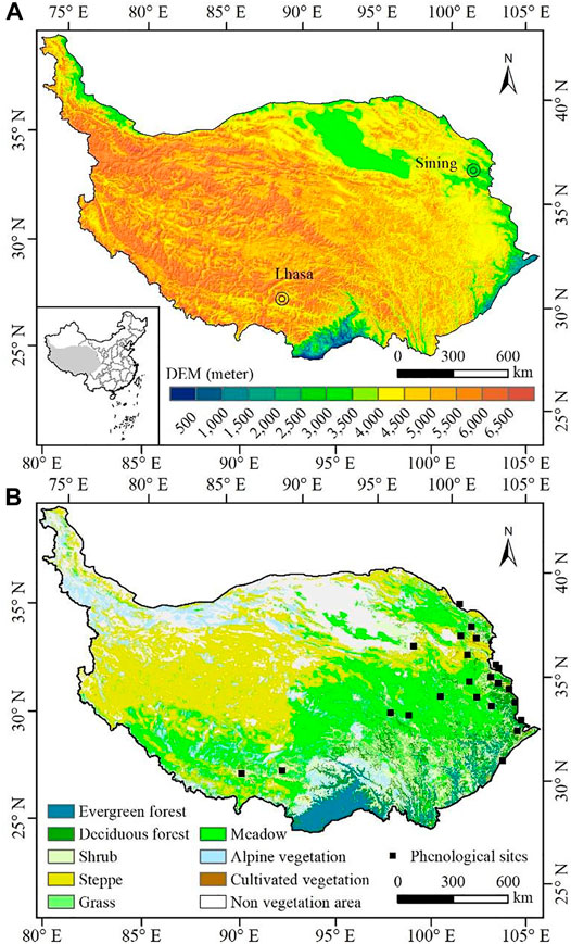
FIGURE 1. (A) Location of the Tibetan Plateau; (B) vegetation-type map redrawn from 1:1,000,000 China vegetation data sets and location of phenological observation stations.

2.2 Data

2.2.1 Satellite-Derived Vegetation Index Datasets

The time series NDVI, EVI, and NDPI data were used to extract the phenological metrics in this paper. The 16-day interval vegetation index datasets containing NDVI and EVI with a spatial resolution of 500 m from 2001 to 2017 were derived from the MODIS/Terra MOD13A1 Version 6 product, which can be obtained from the Land Processes Distributed Active Archive Center (LP DAAC) of the National Aeronautics and Space Administration’s (NASA) Earth Observing System Data and Information System (EOSDIS) (https://lpdaac.usgs.gov/). A series of the sophisticated algorithm (constrained view angle-maximum value composite algorithm, etc.) and strict quality control (low clouds, low view angle, and the highest NDVI/EVI value) were performed in the process of data production to reduce the effect of clouds, solar zenith angles, stratospheric aerosol, etc.

The time series of SR data from MOD09A1 Version 6 product were used to calculate the NDPI, as shown in Eqs. 1, 2, 3. The MOD09A1 product provided an estimate of the surface spectral reflectance of Terra MODIS bands 1 through 7 systematically corrected for atmospheric conditions such as gasses, aerosols, and Rayleigh scattering. The temporal resolution of MOD09A1 is 8 days, and the spatial resolution is 500 m. These data are also freely distributed through the LP DAAC. In this study, surface reflectance in the red (band 1, 620–670 nm), near-infrared (NIR: 841–876 nm, band 2), and short-wave infrared band (SWIR: 1,628–1,652 nm, band 6) during 2001 and 2017 necessary to calculate NDPI were extracted.

$NDPI=\frac{{\rho }_{NIR}-{\rho }_{red}^{SWIR}}{{\rho }_{NIR}+{\rho }_{red}^{SWIR}}(1)$

${\rho }_{red}^{SWIR}=\alpha \times {\rho }_{red}+\left(1-\alpha \right)\times {\rho }_{SWIR}(2)$

$\begin{array}{l}NDPI=\frac{{\rho }_{NIR}-\left(\alpha \times {\rho }_{red}+\left(1-\alpha \right)\times {\rho }_{SWIR}\right)}{{\rho }_{NIR}+\left(\alpha \times {\rho }_{red}+\left(1-\alpha \right)\times {\rho }_{SWIR}\right)}\\ =\frac{{\rho }_{NIR}-\left(0.74\times {\rho }_{red}+0.26\times {\rho }_{SWIR}\right)}{{\rho }_{NIR}+\left(0.74\times {\rho }_{red}+0.26\times {\rho }_{SWIR}\right)}\end{array}(3)$

2.2.2 Vegetation-Type Data

Information of the vegetation distribution in the plateau was derived from the digitized vegetation datasets of China with a scale of 1:1,000,000, published by the Institute of Geography Science and Natural Sources Research, Chinese Academy of Sciences in 2001 (http://www.geodata.cn/Portal/), which was used to identify the vegetation coverage over pixels, as shown in Figure 1B. Due to the lack of seasonality in vegetation index signal, EF mostly in the southeast is not included in our study. We assumed that there were no changes in the vegetation types and distributions on the plateau during the study period as previous studies had done.

2.2.3 Ground-Observed Phenological Data

The ground phenological observations provided by the China Meteorological Administration (CMA, http://cdc.cma.gov.cn) were taken as the true values to validate the accuracy of the phenological products. However, the ground-based phenology was observed in a number of individual plants, while the remote sensing phenology represented the integrated phenological characteristics of a plant community in one pixel. Ground validation of remote sensing measurements with coarse resolution entails considerable difficulties. To improve the reliability of the statistical analysis based on ground observations, ground phenological observations meeting the following requirements (Wang et al., 2017c) were selected: 1) Data integrity—the selected ground sites should have phenological phase continuity and few missing records. 2) Spatial representation—the vegetation type of dominant species at one site must be the same with remote sensing data. The ground phenological observations were selected according to the above requirements, and the information and spatial distribution of phenological sites are shown in Figure 1 and Table 1.

TABLE 1

TABLE 1. Summary of ground phenological observation sites in TP.

2.2.4 Topographic Data

The Shuttle Radar Topography Mission (SRTM) digital elevation model (DEM) data with a spatial resolution of 90 m distributed free of charge was acquired from the Consortium for Spatial Information of the Consultative Group for International Agricultural Research (CGIAR-CSI, http://www.cgiar-csi.org). In this work, the SRTM DEM was used to describe the terrain characteristics. The elevation of each ground phenological site was obtained from the center pixel based on the geolocation information of the ground sites. Furthermore, the relief amplitude and mean slope were extracted from the 3.0 × 3.0-pixel area centered on the phenological sites.

2.3 Data Pre-Processing

Although the effects of satellite orbit shift; solar zenith angles; and atmospheric contaminations of clouds, aerosols, etc. had been systematically corrected from the vegetation index datasets, the time series VI curves still remained jagged because of the residual contamination (Ding et al., 2016; Cong et al., 2017; Chu et al., 2021). The abnormally high and low values existed in the VI trajectories may result in errors and confound retrievals of vegetation phenology (Wang et al., 2015b; Chang et al., 2016). Therefore, the adaptive Savitzky–Golay (S-G) filtering procedure was performed to reduce residual noises in the time series VI datasets by smoothing the VI time series curve, and high-quality NDVI time series datasets were reconstructed (Chang et al., 2016). The adaptive S-G filtering method has been proven to be effective in rebuilding time series from which vegetation phenological metrics can be extracted. The related noise reduction parameters were selected empirically as described in previous studies, which were as follows: spike method = 1, iteration time = 3, adaption strength = 5, and smoothing window = 3, respectively (Borges et al., 2014).

In order to focus on the areas with vegetation and seasonality and to further reduce the impacts of soil variations in bare and sparsely vegetated areas on vegetation, pixels simultaneously satisfying the following criteria were selected: 1) The multiyear average NDVI during growing season (from April to October) should be greater than 0.1. 2) The annual maximum NDVI should be higher than 0.15 and occur between July and September (Piao et al., 2011; Jin et al., 2013; Shen et al., 2014b; Wang et al., 2018). Pixels with lower NDVI value were often considered photosynthetically inactive in land surface phenology, and they could not reveal regular growth cycles along the trajectories and were usually regarded as bare soil or sparsely vegetated lands (Wang et al., 2015a; Wang et al., 2015b). These pixels were masked in the vegetation index datasets and excluded in the following analysis. Besides, evergreen forests were removed from this study due to the lack of seasonality in vegetation index signal relative to those of the other vegetation types (Zhang et al., 2004; Piao et al., 2011; Zheng and Zhu, 2017).

2.4 Phenology Retrieval Algorithms

In this paper, vegetation phenological metrics were retrieved from each of the three vegetation indices (EVI, NDVI, and NDPI) by adopting each of the two methods, respectively, including SA method and STL trendline crossing method. In general, those methods determine the vegetation SOS (EOS) around the time when VI begins to increase (decrease) in spring or early summer (autumn or early winter). Details of those two methods are given as follows.

2.4.1 Seasonal Amplitude Method

In the SA method, SOS is defined as the date (Julian day of the year, DOY) when the left part of the fitted curve has reached a certain ratio of the seasonal amplitude during the VI rising stage, counted from the base level; EOS is defined similarly, as the DOY for which the right side of the fitted curve has decreased to a certain fraction of the seasonal amplitude during the VI decline stage (Jamali et al., 2015; Jönsson and Eklundh, 2004). The seasonal amplitude is defined as difference between the maximum VI value and the base level for each individual season (Eklundh and Jönsson, 2016; Eklundh and Jönsson, 2017). The VI ratio is defined as follows:

$V{I}_{ratio}=\frac{V{I}_t-V{I}_{base}}{V{I}_{max}-V{I}_{base}}(4)$

$V{I}_{base}=0.5\times \left(V{I}_{minimum left}+V{I}_{minimum right}\right)(5)$

where $V{I}_t$ is the VI value at time t, $V{I}_{max}$ is the annual maximum VI value, and $V{I}_{base}$ is given as the average of the left and right minimum values. In this study, we selected a VI ratio threshold of 0.2 to indicate the SOS and a drop of the VI ratio below 0.6 to show the EOS, as determined by Yu et al. (2010).

Among the various retrieval algorithms, the SA method is relatively less affected by surface snow cover, can effectively avoid the mutual interference caused by different hydrothermal conditions, and has been widely used in the extraction of vegetation phenology.

2.4.2 STL Trendline Crossing Method

The seasonal-trend decomposition algorithm based on locally weighted regression (LOESS), widely known as “STL,” is a filtering procedure for decomposing seasonal time series into three additive components of variation: non-linear trend line, seasonal component of time series, and remainder (B Cleveland et al., 1990; Rojo et al., 2017; Sanchez-Vazquez et al., 2012). The trend component (T_t) is considered as the low-frequency variation in the data together with non-stationary, long-term changes in the levels over the time horizon; the seasonal component (S_t) is the variation in the data at or near the seasonal frequency, which is the repetitive pattern over time; the remainder component (R_t) is defined as the irregular remaining variation in the data after the seasonal and trend components have been removed (Aguilera et al., 2015; Cristina et al., 2016).

The STL method is straightforward to use, and advantages of the STL decomposition include simplicity and speed of computation, responsiveness to non-linear trends, flexibility in identifying a seasonal component that changes over time, and robustness of results that are not distorted by transient outliers (Sanchez-Vazquez et al., 2012; Cristina et al., 2016; Rojo et al., 2017). The STL technique has been widely and successfully applied in many fields, especially in natural sciences, such as ecology, environmental science, hydrology, and water resources science, and more details about the STL method can be found in the literature (Aguilera et al., 2015; B Cleveland et al., 1990; Cristina et al., 2016; Jamali et al., 2015; Lafare et al., 2015; Verbesselt et al., 2010).

In this method, the SOS/EOS occurs when the VI time series curve intersect with the STL trend line.

Based on combination of the above two methods and the three vegetation indices, six products were generated, and they were as follows: EVI-based phenological product using SA (E-SA, SOS_E-SA, and EOS_E-SA), EVI-based phenological product using STL (E-STL, SOS_E-STL, and EOS_E-STL), NDVI-based phenological product using SA (N-SA, SOS_N-SA, and EOS_N-SA), NDVI-based phenological product using STL (N-STL, SOS_N-STL, and EOS_N-STL), NDPI-based phenological product using SA (P-SA, SOS_P-SA, and EOS_P-SA), and NDPI-based phenological product using STL (P-STL, SOS_P-STL, and EOS_P-STL).

2.5 Classification of Terrain Complexity

According to the definition of mountainous regions from the United Nations Environment World Conservation Monitoring Centre (UNEP-WCMC) (Kapos, 2000) and relative studies in the literature (Zhang W. et al., 2013; Xie et al., 2019), the degree of terrain complexity was defined using the altitude, relief amplitude, and slope. Then, the topographic conditions were classified into complex terrain if one of the following three criteria was satisfied: 1) when the altitude was lower than 500 m and the relief amplitude exceeds 100 m, 2) when the altitude ranged from 500 to 2,500 m and the relief amplitude exceeds 300 m or slope exceeds 5°, and 3) when the altitude was higher than 2,500 m and the relief amplitude exceeds 500 m or slope exceeds 10°. Otherwise, the topographic conditions were classified into flat terrain.

2.6 Methods for Evaluating the Phenological Products

The difference of the six products was compared comprehensively over the same spatial extent and temporal span: first, at validity containing the missing rate and temporal and spatial stabilities and second at accuracy validation of the retrievals.

The average phenological metrics for each pixel of each product were calculated as the spatial pattern of the TP, and missing rate was calculated as the ratio of all missing pixel counts to the total pixel counts that should be retrieved (Wang et al., 2017b; Wang et al., 2017c; Shang et al., 2018).

Temporal stability means that the inter-annual growth characteristics of vegetation in the same location are similar to some extent as the climatic factors that affect the growth of vegetation (such as temperature, precipitation, etc.) do not change dramatically in the same area (Wang et al., 2017b). Here, the coefficient of variance (CV) (Eq 6) of phenological metric was used as an indicator to describe the temporal stability of each product. The lower the CV was, the more stable the product was at time scale.

$CV=\frac{\sigma }{\mu }(6)$

where $\text{σ}$ is the standard deviation of phenological metric within 2001 and 2017, and $\mu$ is the average value of phenological metric within 17 years.

Spatial stability means that the phenological characteristics of the same vegetation type growing in the same region in 1 year are supposed to be more similar because the meteorological conditions are nearly the same, which means the growth of vegetation should be synchronous in a small window (Tobler, 1970; Wang et al., 2017b; Shang et al., 2018). Here, we use the CV (Eq 6) of phenological metric within a window (3 × 3) to indicate the spatial stability of each product. The greater the CV was, the lower the stability of the product.

$CV=\frac{\sigma }{\mu }(7)$

where $\text{σ}$ is the standard deviation of phenological metric within the window, and $\mu$ is the average value of phenological metric within the window.

In addition, the phenological metrics of products through retrieval algorithms using three satellite-derived VI datasets were validated against ground-observed phenology, respectively (Zheng and Zhu, 2017). The average value of a 3 × 3 window centered at each ground site was extracted as the final result for comparison with the ground-observed phenology. The mean absolute error (MAE) and root mean square error (RMSE) between remote sensing phenological estimations and ground observations were adopted as validation indicators (Wang et al., 2017c; Liu et al., 2017; Guan et al., 2021), as shown in Eqs 8 and 9.

$MAE=\frac{{{\displaystyle \sum }}_{i=1}^n(\left|P{\left(rs\right)}_i-P{\left(site\right)}_i\right|}{n}(8)$

$RMSE=\sqrt{\frac{{{\displaystyle \sum }}_{i=1}^n{\left(P{\left(rs\right)}_i-P{\left(site\right)}_i\right)}^2}{n}}(9)$

where $P{\left(rs\right)}_i$ is the satellite-derived phenological date at year i, $P{\left(site\right)}_i$ is the ground observation at year i, and n is the number of years.

3 Results and Analysis

3.1 Comparison of Phenological Products at Regional Scales

Figure 2 presents the mean SOS for the TP during 2001–2017 derived from the six products. In general, inconsistencies of SOS derived from different VI datasets using different methods existed and varied in different areas. The SOS derived from the same VI using different algorithms had consistent patterns in the west, but inconsistent patterns were exhibited in the east. The SOS based on SA (Figure 2A, C, E) in the east was 5–15 days earlier than that based on STL (Figure 2B, D, F) from the same VI dataset. The SOS derived from different VI using the same method have consistent patterns in the east, but inconsistent patterns were exhibited in the middle and northwest. The SOS from NDVI (Figure 2C, D) in the middle was 5–10 days earlier than that from EVI (Figure 2A, B), while the SOS from NDPI (Figure 2E, F) in the northwest was 10–20 days earlier than that from EVI.

FIGURE 2

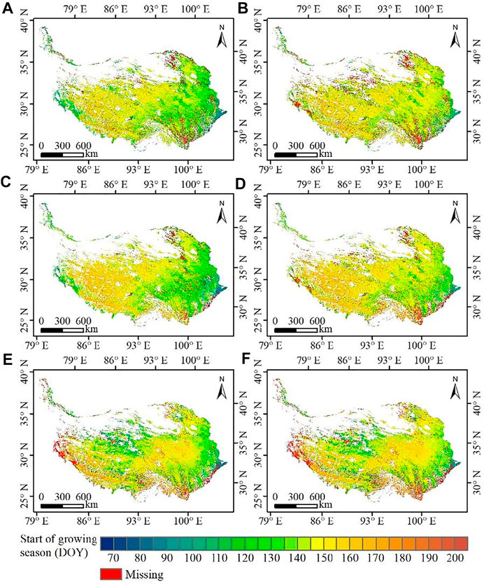
FIGURE 2. Spatial pattern of mean start of season (SOS) between (A) E-SA, (B) E-STL, (C) N-SA, (D) N-STL, (E) P-SA, and (F) P-STL.

For each product, various degrees of differences among the multi-year average EOS for the TP from 2001 to 2017 are found in Supplementary Figure S1. The EOS derived using STL (Supplementary Figure S1B, D, F) had the same spatial pattern as those using SA (Supplementary Figure S1A, C, E) with the same VI, but was 15–30 days later than that using SA with the same VI in the same area. Also, inconsistencies of EOS derived from different VI using the same method existed and varied in different regions. The EOS from NDVI (Supplementary Figure S1C, D) was 10–30 days later than that from EVI (Supplementary Figure S1A, B) in the south, respectively, while the EOS from NDPI (Supplementary Figure S1E, F) was 5–10 days earlier in the south.

3.1.1 Missing Rate

For the six phenological products, the missing data existed inevitably and varied in different regions. In general, the missing rates of SOS in E-SA, E-STL, N-SA, N-STL, P-SA, and P-STL were 7.38%, 10.6%, 4.58%, 8.3%, 7.11%, and 9.25%, respectively, as shown in and Figures 2 and 3. For the same VI source, the missing rate of SOS based on STL was higher than that based on SA; for the same retrieval algorithm, the missing rate of SOS derived from NDVI was the lowest, then the NDPI, and the missing rate of SOS derived from EVI was the highest (Figure 3). Figure 3 presents the missing rates of the six products in different vegetation types. For SOS (Figure 3), the missing rate was the lowest or relatively lower in the meadow (E-SA: 5.06%, E-STL: 6.83%, N-SA: 4.08%, N-STL: 7.04%, P-SA: 3.99%, and P-STL: 5.46%), but the relatively higher or the highest missing rates of the six products existed in different vegetation types; for SOS from EVI and NDVI, the missing rate was relatively higher in DF (E-SA: 18.03%, E-STL: 20.49%, N-SA: 7.72%, and N-STL: 16.49%); for SOS from NDPI, the missing rate was the highest in AV (P-SA: 17.34% and P-STL: 21.84%).

FIGURE 3

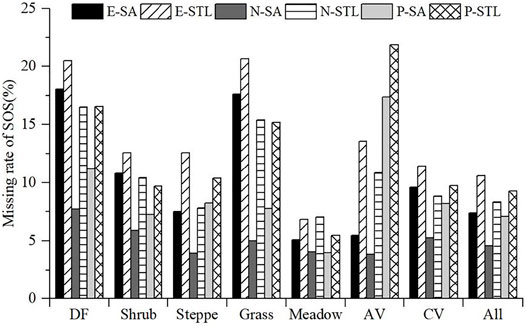
FIGURE 3. Missing rates of SOS over different vegetation types.

As displayed in Supplementary Figures S1 and S2, the overall missing rates of EOS in E-SA, E-STL, N-SA, N-STL, P-SA, and P-STL were 7.82%, 17.53%, 6%, 18.51%, 12.96%, and 29.21%, respectively. For the same VI source, the missing rate of EOS based on STL was twice more than that based on SA; for the same retrieval algorithm, the missing rate of EOS derived from NDVI was still the lowest, different from SOS; EOS with the highest missing rate was derived from EVI. Similar to SOS, EOS of the six products (Supplementary Figure S2) in meadow had the lowest missing rate (E-SA: 4.73%, E-STL: 6.83%, N-SA: 4.59%, N-STL: 13.43%, P-SA: 6.92%, and P-STL: 20.13%), and the highest missing rate was in DF from NDVI or EVI (E-SA: 18.54%, E-STL: 29.59%, N-SA: 13.41%, and N-STL: 37.20%) and in AV from NDPI (P-SA: 19.49% and P-STL: 45.46%).

In addition, the missing rates of phenological metrics from the six products at different degrees of terrain complexity were compared. As shown in Figure 4, the missing rates of SOS from the six products at the complex terrain were larger than those at the flat terrain. Over the flat terrain, the missing rates of SOS in E-SA, E-STL, N-SA, N-STL, P-SA, and P-STL were 4.89%, 9.14%, 4.13%, 7.20%, 4.82%, and 6.39%, respectively; over the complex terrain, the missing rates of SOS in E-SA, E-STL, N-SA, N-STL, P-SA, and P-STL were 9.21%, 12.29%, 5.01%, 9.57%, 9.17%, and 11.70%, respectively. In addition, EOS at the complex terrain also showed higher missing rates than the flat terrain (Supplementary Figure S3). The missing rates of EOS in E-SA, E-STL, N-SA, N-STL, P-SA, and P-STL over the flat terrain were 5.31%, 15.20%, 4.48%, 14.20%, 11.61%, and 27.23%, respectively, and the missing rates of EOS in E-SA, E-STL, N-SA, N-STL, P-SA, and P-STL over the complex terrain were 9.99%, 20.83%, 7.53%, 23.14%, 14.62%, and 31.44%, respectively.

FIGURE 4

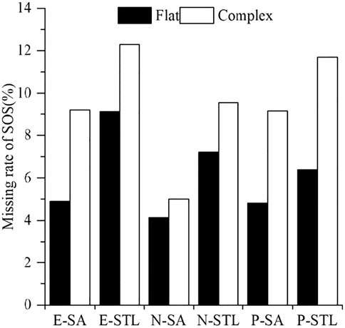
FIGURE 4. Comparison of missing rates of SOS over the flat terrain and the complex terrain.

The high spatial variations in geographic configurations caused by obvious topographic conditions over the complex terrain may affect the quality of input VI data for phenological extractions and then lead to higher missing rates of phenological metrics compared with the flat terrain.

3.1.2 Temporal Stability

Table 2 shows the temporal stabilities of SOS from 2001 to 2017 using CV as indicator. In general, the SOS derived from EVI or NDVI had higher temporal stabilities than those from NDPI for each method, and SOS based on the SA method were a little more stable than those based on the STL method for each vegetation index. Specifically, the SOS from E-SA, E-STL, N-SA, and N-STL product had lower CVs (the means and standard deviations were 0.147 ± 0.112, 0.148 ± 0.103, 0.137 ± 0.098, and 0.141 ± 0.092, respectively) than those from P-SA and P-STL product (the means and standard deviations were 0.191 ± 0.146, 0.192 ± 0.149, respectively). Besides, the temporal stabilities of SOS varied among different vegetation types, as shown in Table 2. For DF, shrub, and CV types, the SOS from E-SA were superior to those from others in the aspect of temporal stability, with the lowest CVs of 0.160 ± 0.124, 0.130 ± 0.104, and 0.111 ± 0.087, respectively, followed by the SOS from E-STL, with CVs of 0.162 ± 0.105, 0.138 ± 0.092, and 0.124 ± 0.081, respectively. For steppes, SOS_N-SA and SOS_N-STL had better temporal stabilities compared with others, with CVs of 0.133 ± 0.091 and 0.131 ± 0.095, respectively. However, for grass, SOS_E-SA and SOS_E-STL were relatively more stable, with CVs of 0.190 ± 0.117 and 0.190 ± 0.106, respectively. For meadows, SOS_N-SA was the most stable, followed by SOS_E-SA and SOS_N-STL, with CVs of 0.122 ± 0.091, 0.127 ± 0.103, and 0.130 ± 0.084, respectively. For AVs, the CV of SOS_N-SA was the lowest, with CV of 0.170 ± 0.094, followed by SOS_E-SA and SOS_N-STL, with CVs of 0.187 ± 0.110 and 0.194 ± 0.104, respectively.

TABLE 2

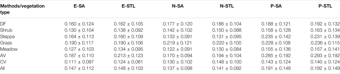
TABLE 2. The means and standard deviations of SOS CV for different vegetation types from 2001 to 2017.

Supplementary Table S1 presents the temporal stabilities of EOS from 2001 to 2017 using CV as an indicator. In general, the temporal stabilities of EOS were slightly different from SOS. Differences existed between EOS based on the SA method and the STL method for each vegetation index in the aspect of temporal stability; EOS based on STL (EOS_E-STL: 0.070 ± 0.042, EOS_N-STL: 0.044 ± 0.023, and EOS_P-STL: 0.051 ± 0.032) had higher CVs than those based on SA (EOS_E-SA: 0.037 ± 0.018, EOS_N-SA: 0.037 ± 0.018, and EOS_P-SA: 0.046 ± 0.028). Besides, the temporal stabilities of EOS varied among different vegetation types, as shown in Supplementary Table S1. For DF, shrub, grass, and CV types, EOS_E-SA, EOS_N-SA, and EOS_P-SA had higher temporal stabilities than others, as their CVs were lower than others. For steppe, meadow, and AV types, EOS_E-SA and EOS_N-SA were more stable than others, with lower CVs.

Table 3 shows temporal stability comparisons of satellite-derived SOS over the flat terrain and the complex terrain. The SOS over complex the terrain showed lower stabilities than those over the flat terrain. Over the flat terrain, the CV values of SOS from E-SA, E-STL, N-SA, N-STL, P-SA, and P-STL were 0.146 ± 0.111, 0.147 ± 0.100, 0.127 ± 0.092, 0.132 ± 0.092, 0.188 ± 0.153, and 0.192 ± 0.139, respectively. Over the complex terrain, the CV values of SOS from E-SA, E-STL, N-SA, N-STL, P-SA, and P-STL were 0.148 ± 0.113, 0.150 ± 0.106, 0.146 ± 0.103, 0.148 ± 0.092, 0.195 ± 0.138, and 0.199 ± 0.156, respectively. Similar to SOS, the CV values of satellite-derived EOS over the complex terrain were much higher than those over the flat terrain, as shown in Supplementary Table S2. Over the flat terrain, the CV values of SOS from E-SA, E-STL, N-SA, N-STL, P-SA, and P-STL were 0.036 ± 0.017, 0.067 ± 0.040, 0.035 ± 0.016, 0.040 ± 0.019, 0.042 ± 0.026, and 0.051 ± 0.032, respectively. Over the complex terrain, the CV values of EOS from E-SA, E-STL, N-SA, N-STL, P-SA, and P-STL were 0.038 ± 0.019, 0.072 ± 0.043, 0.039 ± 0.019, 0.048 ± 0.026, 0.050 ± 0.029, and 0.056 ± 0.032, respectively.

TABLE 3

TABLE 3. The means and standard deviations of SOS CV for different terrains from 2001 to 2017.

The CV differences of phenological metrics over different terrains on time scale revealed the fact that the complexity of topography could affect the temporal stabilities of retrieved phenological results; the temporal stabilities of retrieved phenological metrics over the flat terrain were more stable than those over the complex terrain.

3.1.3 Spatial Stability

To analyze the spatial stability of each product, a 3 × 3 sliding window was used to search the phenological metrics in the study area, and the CV value of the central point in the window and the same vegetation type in the sliding window was calculated.

The spatial stabilities of SOS are displayed in Table 4. In general, the SOS derived from NDVI had relatively higher spatial stabilities than those from EVI or NDPI for each method, with CVs of 0.040 ± 0.033 and 0.040 ± 0.040, respectively, and the differences of spatial stability were small between SOS based on the SA method and the STL method for each vegetation index. In addition, N-SA and N-STL also performed better in the extraction of SOS for each vegetation type than others, as the CV values of SOS_N-SA and SOS_N-STL for each vegetation type were a little lower than those of others. Among the vegetation types, the spatial stabilities of SOS in meadows, AVs, and CVs were better than other vegetation types, with lower CV values, and the greatest CV values occurred in grass. Following behind grass, the CV values in DFs were relatively larger.

TABLE 4

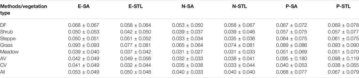
TABLE 4. The means and standard deviations of SOS spatial CV for different vegetation types.

Supplementary Table S3 presents the spatial stabilities of EOS. Similar to SOS, for all vegetation types, the EOS derived from NDVI had relatively better spatial stabilities than those from EVI or NDPI for each method, with CVs of 0.012 ± 0.009 and 0.013 ± 0.012, respectively, and the differences of spatial stability were small between SOS based on the SA method and the STL method for each vegetation index. Besides, EOS from N-SA and N-STL were relatively stable than those from others for each vegetation type, as the CV values of EOS_N-SA and EOS_N-STL for each vegetation type were a little lower than those of others. Among the vegetation types, the EOS in meadows and CVs were a little more stable than other vegetation types, with lower CV values, and the CV values in grass and DFs were relatively larger.

Table 5 presents spatial stability comparisons of satellite-derived SOS over the flat terrain and the complex terrain. The SOS over the complex terrain showed lower stabilities than those over the flat terrain. Over the flat terrain, the CV values of SOS from E-SA, E-STL, N-SA, N-STL, P-SA, and P-STL were 0.032 ± 0.039, 0.032 ± 0.042, 0.024 ± 0.029, 0.025 ± 0.032, 0.039 ± 0.053, and 0.037 ± 0.054, respectively. Over the complex terrain, the CV values of SOS from E-SA, E-STL, N-SA, N-STL, P-SA, and P-STL were 0.050 ± 0.054, 0.046 ± 0.053, 0.037 ± 0.036, 0.038 ± 0.045, 0.067 ± 0.088, and 0.067 ± 0.090, respectively. Similarly, the CV values of satellite-derived EOS over the complex terrain were much higher than those over the flat terrain, as presented in Supplementary Table S4. Over the flat terrain, the CV values of EOS_E-SA, EOS_E-STL, EOS_N-SA, EOS_N-STL, EOS_P-SA, and EOS_P-STL were 0.009 ± 0.010, 0.009 ± 0.010, 0.007 ± 0.007, 0.009 ± 0.009, 0.010 ± 0.013, and 0.012 ± 0.013, respectively. Over the complex terrain, the CV values of EOS_E-SA, EOS_E-STL, EOS_N-SA, EOS_N-STL, EOS_P-SA, and EOS_P-STL were 0.015 ± 0.016, 0.013 ± 0.011, 0.011 ± 0.010, 0.012 ± 0.013, 0.016 ± 0.020, and 0.017 ± 0.021, respectively.

TABLE 5

TABLE 5. The means and standard deviations of SOS spatial CV for different terrains.

The CV differences of phenological metrics over the different terrains on spatial scale revealed the fact that the complexity of topography could affect the spatial stabilities of extracted phenological results, and the spatial stabilities of extracted phenological metrics over the complex terrain were less stable than those over the flat terrain.

3.2 Accuracy Assessment of Satellite-Derived Phenologies Based on Ground Observations

The difference between ground-observed SOS and satellite-derived SOS from the three satellite-derived VIs based on different extraction algorithms is shown in Figure 5. For all vegetation types, the SA-extracted SOS from EVI and NDVI (SOS_E-SA and SOS_N-SA) had better agreements with ground observations than others, with MAEs of 18.95 and 19.60 days year⁻¹, respectively. The differences were smaller for SOS based on the SA method and larger for that based on the STL method; the MAEs of SOS_E-STL, SOS_N-STL, and SOS_P-STL were 4 days higher than those of SOS_E-SA, SOS_N-SA, and SOS_P-SA, respectively. For steppes, the SA-extracted SOS from NDVI and EVI (SOS_N-SA and SOS_E-SA) matched better with ground-observed SOS than others, with MAEs of 23.05 and 25.01 days year⁻¹, respectively. The SA method can extract information of SOS with higher accuracy than the STL method, and the MAEs of SOS_E-STL, SOS_N-STL, and SOS_P-STL were more than 6 days higher than those of SOS_E-SA, SOS_N-SA, and SOS_P-SA, respectively. Of all the vegetation types, the SOS in meadows were closer to the 1:1 line than in other vegetation types, with the lowest MAEs and RMSEs. The correlations between SA-extracted SOS from NDVI and EVI (SOS_N-SA and SOS_E-SA) and ground observations were stronger than others, with MAEs of 10.51 and 12.24 days year⁻¹, respectively. Differences still existed between SOS based on the SA method and the STL method and were similar to those in steppes. At CV sites, SOS based on the SA method matched relatively better with ground-observed SOS than those based on the STL method, but the differences of extraction accuracies between SA and STL were relatively smaller compared with those in other vegetation types.

FIGURE 5

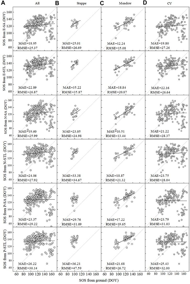
FIGURE 5. Comparison between SOS from E-SA, E-STL, N-SA, N-STL, P-SA, and P-STL for different vegetation types based on the ground observations. (A) All, (B) steppe, (C) meadow, and (D) cultivated vegetation (CV). Gray lines are the 1:1 line, and black lines are the best linear regression line.

Supplementary Figure S4 shows comparisons between EOS from E-SA, E-STL, N-SA, N-STL, P-SA, and P-STL for different vegetation types based on the ground observations. In general, the SA method performed much better than the STL method, either for all vegetation types together or only one of them, as the MAEs of EOS based on STL were about twice and even much more than MAEs of EOS based on SA. Besides, the accuracies of EOS from EVI, NDVI, and NDPI were different for different vegetation types. For all vegetation types, the SA-extracted SOS from NDPI and EVI had better agreements with ground-observed EOS than that from NDVI, and the MAEs of EOS_P-SA and EOS_E-SA were 22.84 and 25.60 days year⁻¹, respectively, while it was 33.72 days year⁻¹ for EOS_N-SA. Of all the vegetation types, the accuracy of EOS in steppes was the highest compared to other vegetation types, with the lowest MAEs and RMSEs, and the accuracies of EOS_P-SA, EOS_N-SA, and EOS_E-SA had little difference in steppes than in others, with MAEs of 8.46, 10.84, and 13.07 days year⁻¹, respectively. For meadows, EOS from P-SA matched best with ground observations (with MAE of 18.41 days year⁻¹), followed by EOS from E-SA (with MAE of 24.24 days year⁻¹), and the accuracy of EOS_N-SA was the lowest among EOS based on the SA method (with MAE of 27.20 days year⁻¹). At CV sites, the correlations between EOS_P-SA, EOS_E-SA, and ground-observed EOS were stronger than EOS_N-SA, with MAEs of 27.16, 27.99, and 36.38 days year⁻¹, respectively.

Figure 6 presents accuracy comparisons of satellite-derived SOS over the flat terrain and complex terrain. The complex terrain showed lower accuracy of satellite-derived SOS (MAE = 31.79 days year⁻¹) than the flat terrain (MAE = 20.67 days year⁻¹). Over the flat terrain, the MAE values between SOS from E-SA, E-STL, N-SA, N-STL, P-SA, and P-STL and ground-observed SOS were 16.23 ± 11.65 days year⁻¹, 22.17 ± 13.52 days year⁻¹, 16.8 ± 12.19 days year⁻¹, 23.21 ± 14.13 days year⁻¹, 20.5 ± 13.49 days year⁻¹, and 25.13 ± 14.22 days year⁻¹, respectively. Over the complex terrain, the MAE values between SOS from E-SA, E-STL, N-SA, N-STL, P-SA, and P-STL and ground-observed SOS were 32.63 ± 28.42 days year⁻¹, 26.48 ± 16.07 days year⁻¹, 33.48 ± 27.65 days year⁻¹, 28.21 ± 13.61 days year⁻¹, 38.14 ± 26.32 days year⁻¹, and 31.80 ± 16.72 days year⁻¹, respectively. Similarly, the MAE values between satellite-derived EOS and ground EOS over the complex terrain (mean = 49.97 days year⁻¹) were much higher than those over the flat terrain (mean = 39.08 days year⁻¹), as presented in Supplementary Figure S5. Over the flat terrain, the MAE values between EOS from E-SA, E-STL, N-SA, N-STL, P-SA, and P-STL and ground-observed EOS were 24.68 ± 21.09 days year⁻¹, 52.38 ± 22.94 days year⁻¹, 28.44 ± 22.87 days year⁻¹, 59.65 ± 24.32 days year⁻¹, 20.11 ± 20.02 days year⁻¹, and 49.22 ± 24.85 days year⁻¹, respectively. Over the complex terrain, the MAE values between EOS from E-SA, E-STL, N-SA, N-STL, P-SA, and P-STL and ground-observed EOS were 28.79 ± 16.01 days year⁻¹, 60.91 ± 19.57 days year⁻¹, 42.94 ± 15.97 days year⁻¹, 72.30 ± 21.13 days year⁻¹, 32.24 ± 14.29 days year⁻¹, and 62.61 ± 20.27 days year⁻¹, respectively.

FIGURE 6

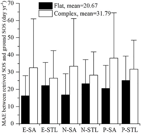
FIGURE 6. Comparison of mean absolute error (MAE) values of SOS over the flat terrain and the complex terrain.

The larger MAE values between phenological metrics and ground observations over the complex terrain revealed the fact that the extraction of phenological metrics over the complex terrain had larger disagreements with ground observations than those over the flat terrain, and it can be concluded that the complex terrain had a larger influence on extraction accuracy than the flat terrain.

4 Discussion

4.1 Comparison of Different Methods Using Different VI Datasets in Phenological Metric Extractions

The time series of satellite-derived VI datasets have made it possible to study the vegetation phenology and its interactions with surrounding environment conditions for a long time at large scale (An et al., 2018; Wang and Wu, 2019). The time series VI datasets, together with phenological retrieval algorithms, could affect the vegetation phenological metrics, but few evaluations are performed. In this study, we employed two methods using three VI datasets to retrieve the vegetation phenological metrics in the TP, and the effectiveness of each result was evaluated.

It is shown that the missing rates of phenological metrics (Figure 3; Supplementary Figure S2) based on SA for each VI were lower than those based on STL; as the vegetation index value was relatively lower in the TP, the seasonal trend line may not cross with part of the vegetation index time series curve and then lead to missing of phenological metrics. Besides, phenological metrics derived from NDVI had lower missing rates than other VIs. However, the missing rates of EOS were higher than those of SOS, which were mainly because the DOY of EOS were more likely to be larger than 365 in the process of retrieval and thus treated as an invalid value.

In general, the phenological metrics based on SA for each VI were a little more stable than those based on STL in the aspect of temporal stability, and the phenological metrics derived from NDVI had higher temporal stabilities than those from EVI or NDPI (Table 2; Supplementary Table S1). However, for the DFs, shrubs, grass, and CVs, SOS derived from EVI were superior to those from others. In addition, EOS based on STL were much more unstable than those based on SA, and SOS derived from NDVI or EVI had higher temporal stabilities than those from NDPI. The higher CV values of SOS for each vegetation type than those of EOS meant that the SOS varied greater than EOS during the study period and was more sensitive to environmental factors, which was almost consistent with the study of Wang et al. (2019).

As for the spatial stability (Table 4; Supplementary Table S3), phenological metrics derived from NDVI had relatively better spatial stabilities than those from EVI or NDPI for each method, and the differences of spatial stability were relatively small between phenological metrics based on the SA method and the STL method for each vegetation index. The higher spatial CV values of SOS than EOS indicated that the differences of SOS in different regions for each vegetation type were larger than those of EOS.

The accuracy assessment based on ground observations (Figure 5; Supplementary Figure S4) in this paper shows that phenological metrics based on SA had better agreements with ground observations than those based on STL for each VI, as MAEs between phenological metrics based on SA and ground observations were much lower than those between phenological metrics based on STL and ground observations, implying that the SA method was more suitable to monitor phenology on the TP. The same conclusion was also found in previous studies (Yu et al., 2010; Zheng and Zhu, 2017). Moreover, smaller MAEs and RMSEs were found between SOS_E-SA, as well as SOS_N-SA, and ground-observed SOS, indicating that NDVI or EVI might be more consistent than NDPI with the ground-observed SOS. EVI or NDVI may be more appropriate for monitoring SOS than NDPI in the TP. However, regarding EOS, smaller MAEs and RMSEs between EOS_P-SA and ground-observed EOS were found for all the vegetation types. However, more ground-observed phenological records are needed to confirm it due to only fewer available sites mainly in the east of the TP in our study. When compared with SOS, EOS is much difficult to be monitored (Liu et al., 2016; Jeong et al., 2017; Wu et al., 2017; Zheng and Zhu, 2017) as the MAEs were larger between derived EOS and ground-observed EOS than those between derived SOS and ground-observed SOS. However, it was opposite for the steppes, which was probably due to the relatively lower vegetation coverage in these areas, and it was difficult to capture the greenness change of vegetation as it was likely to be affected by the background of soil.

4.2 The Topographic Effect on Phenological Estimations

As the complex terrain usually present high spatial heterogeneity, the satellite-derived phenology results in complex areas displayed more uncertainties than those in flat areas. In this study, we have checked the topographic influence on retrieved phenological metrics. The results showed that phenological metrics over the complex terrain had higher missing rates than those over the flat terrain (Figures 2 and 4; Supplementary Figures S1 and S3). In addition, the phenological results over the complex terrain were more unstable at the temporal and spatial scale than those over the flat terrain (Tables 3 and 5; Supplementary Tables S2 and S4). Besides, the phenological metrics over the complex terrain also had larger disagreements with ground observations than those over the flat terrain (Figure 6; Supplementary Figure S5). The high spatial variations in geographic configurations caused by obvious topographic conditions may cause sustainable and complex uncertainties in the surface reflectance data, then may affect the quality of input VI data for phenological extractions, and then lead to higher uncertainties of phenological metrics compared with the flat terrain (Jin et al., 2017; Xie and Li, 2020b). As terrain gradients usually result in frequent changes of local climate, the surface reflectance data over the complex terrain is more susceptible to external environmental conditions. The surface reflectance data over the complex terrain is more likely to be contaminated by clouds, aerosols, snow, etc. (Xie et al., 2019). The increasing angular variations between the sun and satellite over the complex terrain may lead to more complicated solar irradiances than those over the flat terrain (Yan et al., 2018; Xie et al., 2021a).

Nevertheless, the topographical effects tend to be ignored (Jin et al., 2017) by most of the current retrieval methods for phenological extractions and then lead to more uncertainties into the phenological metrics. In this work, the lower missing rates, better stabilities on the temporal and spatial scale, and higher accuracies in phenological metrics were found over the flat terrain than the complex terrain; thus, the retrieval work of phenological metrics over the complex terrain is more challenging than that over the flat terrain (Xie et al., 2018).

4.3 Deficiencies in Ground Observations

Accuracy assessment using ground observations is always an important concern in any remote sensing-based monitoring and analysis, especially at a large scale (Wang et al., 2017c; Shen et al., 2021). However, the limitations of ground-observed validation data in the TP and the inconsistency and scale effect between remote sensing results and observations at ground sites make it difficult to validate large-scale remote sensing monitoring results by using ground-observed data (Wang et al., 2017b). Due to the limitations of ground-observed validation data in the TP, the accuracy assessment of this study only considers the vegetation types of steppe, CV, and meadow mainly in the east. In the future research, it is necessary to continue to expand the area and consider more vegetation types to conduct a more comprehensive precision evaluation of phenological products. It is worth noting that retrieved phenological metrics were derived from 500-m, 16-day composite NDVI/EVI or 8-day composite NDPI data, while ground observations are daily point-based observations. The remote sensing phenological metrics are based upon greenness of a pixel, while ground observations rely on the morphological changes of individual plants; thus, inconsistencies exist between them as different species at the same stage could exhibit different greenness because of differences in the characteristic area of individual leaves (Shen et al., 2015; Wang et al., 2017c). Although the studied sites are the best representation for each station and the surrounding area, a great number of species that exhibit diverse phenological stages coexist within a pixel, and the scale effect of incomplete match between ground site and remote sensing pixel at the temporal and spatial scales is unavoidable (Wang et al., 2017c). All these might lead to disagreements between retrieved phenological metrics and ground observations.

5 Conclusion

In this study, vegetation phenological metrics in the TP were derived based on different extraction algorithms using three satellite-derived vegetation indices, and comparative analyses of the results were conducted in different aspects. We found that the SA method performed better than STL in the extraction of phenological metrics, as phenological metrics based on SA had lower missing rate, better stability on the temporal and spatial scales, and better agreements with ground observations. Meanwhile, the EVI, NDVI, and NDPI had advantages in different aspects. Different retrieving approaches may produce significantly different estimates of SOS and EOS, with VI differences also accounting for differences. Besides, the results also showed that the complex terrain had larger influence on extraction accuracy than the flat terrain, and extraction of phenological metrics over the complex terrain was more challenging than that over the flat terrain. Furthermore, given present approaches and datasets, substantial room for improvement exists for using remote sensing applications to predict ecosystem phenology at broad spatial scales. It should be considered that uniting multisource data is an effective way to improve the accuracy and validity of remote sensing phenological products. Different combinations of datasets and retrieval methods may need to be applied for different plant functional types, and in particular, identifying the specific best settings to each ecosystem type will be a future research challenge. These findings are of great value for improving the spatial resolution of remote sensing phenological products to promote their application and development in the future.

Data Availability Statement

The original contributions presented in the study are included in the article/Supplementary Material; further inquiries can be directed to the corresponding author.

Author Contributions

All authors listed have made a substantial, direct, and intellectual contribution to the work and approved it for publication.

Funding

This work was sponsored by the National Natural Science Foundation of China (Grant No. 31870708 and 51879155).

Conflict of Interest

The authors declare that the research was conducted in the absence of any commercial or financial relationships that could be construed as a potential conflict of interest.

Publisher’s Note

All claims expressed in this article are solely those of the authors and do not necessarily represent those of their affiliated organizations, or those of the publisher, the editors, and the reviewers. Any product that may be evaluated in this article, or claim that may be made by its manufacturer, is not guaranteed or endorsed by the publisher.

Supplementary Material

The Supplementary Material for this article can be found online at: https://www.frontiersin.org/articles/10.3389/fenvs.2021.794189/full#supplementary-material

References

Aguilera, F., Orlandi, F., Ruiz-Valenzuela, L., Msallem, M., and Fornaciari, M. (2015). Analysis and Interpretation of Long Temporal Trends in Cumulative Temperatures and Olive Reproductive Features Using a Seasonal Trend Decomposition Procedure. Agric. For. Meteorol. 203, 208–216. doi:10.1016/j.agrformet.2014.11.019

CrossRef Full Text | Google Scholar

An, S., Zhu, X., Shen, M., Wang, Y., Cao, R., Chen, X., et al. (2018). Mismatch in Elevational Shifts between Satellite Observed Vegetation Greenness and Temperature Isolines during 2000-2016 on the Tibetan Plateau. Glob. Change Biol. 24, 5411–5425. doi:10.1111/gcb.14432

PubMed Abstract | CrossRef Full Text | Google Scholar

Araya, S., Lyle, G., Lewis, M., and Ostendorf, B. (2016). Phenologic Metrics Derived from MODIS NDVI as Indicators for Plant Available Water-Holding Capacity. Ecol. Indic. 60, 1263–1272. doi:10.1016/j.ecolind.2015.09.012

CrossRef Full Text | Google Scholar

B Cleveland, R., Cleveland, S. W., E McRae, J., and Terpenning, I. (1990). STL: A Seasonal-Trend Decomposition Procedure Based on Loess. J. Official Stat. 6, 3–33.

Google Scholar

Borges, E. F., Sano, E. E., and Medrado, E. (2014). Radiometric Quality and Performance of TIMESAT for Smoothing Moderate Resolution Imaging Spectroradiometer Enhanced Vegetation index Time Series from Western Bahia State, Brazil. J. Appl. Remote Sens. 8, 083580. doi:10.1117/1.jrs.8.083580

CrossRef Full Text | Google Scholar

Cao, R., Chen, J., Shen, M., and Tang, Y. (2015). An Improved Logistic Method for Detecting spring Vegetation Phenology in Grasslands from MODIS EVI Time-Series Data. Agric. For. Meteorol. 200, 9–20. doi:10.1016/j.agrformet.2014.09.009

CrossRef Full Text | Google Scholar

Chang, Q., Zhang, J., Jiao, W., Yao, F., and Wang, S. (2016). Spatiotemporal Dynamics of the Climatic Impacts on greenup Date in the Tibetan Plateau. Environ. Earth Sci. 75, 1343. doi:10.1007/s12665-016-6148-6

CrossRef Full Text | Google Scholar

Chu, D., Shen, H., Guan, X., Chen, J. M., Li, X., Li, J., et al. (2021). Long Time-Series NDVI Reconstruction in Cloud-Prone Regions via Spatio-Temporal Tensor Completion. Remote Sens. Environ. 264, 112632. doi:10.1016/j.rse.2021.112632

CrossRef Full Text | Google Scholar

Cong, N., Shen, M., Piao, S., Chen, X., An, S., Yang, W., et al. (2017). Little Change in Heat Requirement for Vegetation green-up on the Tibetan Plateau over the Warming Period of 1998-2012. Agric. For. Meteorol. 232, 650–658. doi:10.1016/j.agrformet.2016.10.021

CrossRef Full Text | Google Scholar

Cristina, S., Cordeiro, C., Lavender, S., Costa Goela, P., Icely, J., and Newton, A. (2016). MERIS Phytoplankton Time Series Products from the SW Iberian Peninsula (Sagres) Using Seasonal-Trend Decomposition Based on Loess. Remote Sens. 8, 449. doi:10.3390/rs8060449

CrossRef Full Text | Google Scholar

Ding, M., Chen, Q., Li, L., Zhang, Y., Wang, Z., Liu, L., et al. (2016). Temperature Dependence of Variations in the End of the Growing Season from 1982 to 2012 on the Qinghai-Tibetan Plateau. GIScience Remote Sens. 53, 147–163. doi:10.1080/15481603.2015.1120371

CrossRef Full Text | Google Scholar

Duveiller, G., Weiss, M., Baret, F., and Defourny, P. (2011). Retrieving Wheat Green Area Index during the Growing Season from Optical Time Series Measurements Based on Neural Network Radiative Transfer Inversion. Remote Sens. Environ. 115, 887–896. doi:10.1016/j.rse.2010.11.016

CrossRef Full Text | Google Scholar

Eklundh, L., and Jönsson, P. (2016). “TIMESAT for Processing Time-Series Data from Satellite Sensors for Land Surface Monitoring,” in Multitemporal Remote Sensing: Methods and Applications. Editor Y. Ban (Cham: Springer International Publishing), 177–194. doi:10.1007/978-3-319-47037-5_9

CrossRef Full Text | Google Scholar

Eklundh, L., and Jönsson, P. (2017). TIMESAT 3.3 with Seasonal Trend Decomposition and Parallel Processing Software Manual. Sweden: Lund University.

Google Scholar

Gamon, J. A., Huemmrich, K. F., Stone, R. S., and Tweedie, C. E. (2013). Spatial and Temporal Variation in Primary Productivity (NDVI) of Coastal Alaskan Tundra: Decreased Vegetation Growth Following Earlier Snowmelt. Remote Sens. Environ. 129, 144–153. doi:10.1016/j.rse.2012.10.030

CrossRef Full Text | Google Scholar

Guan, X., Chen, J. M., Shen, H., and Xie, X. (2021). A Modified Two-Leaf Light Use Efficiency Model for Improving the Simulation of GPP Using a Radiation Scalar. Agric. For. Meteorol. 307, 108546. doi:10.1016/j.agrformet.2021.108546

CrossRef Full Text | Google Scholar

Han, G., and Xu, J. (2013). Land Surface Phenology and Land Surface Temperature Changes along an Urban-Rural Gradient in Yangtze River Delta, China. Environ. Manage. 52, 234–249. doi:10.1007/s00267-013-0097-6

PubMed Abstract | CrossRef Full Text | Google Scholar

Jamali, S., Jönsson, P., Eklundh, L., Ardö, J., and Seaquist, J. (2015). Detecting Changes in Vegetation Trends Using Time Series Segmentation. Remote Sens. Environ. 156, 182–195. doi:10.1016/j.rse.2014.09.010

CrossRef Full Text | Google Scholar

Jeong, S.-J., Schimel, D., Frankenberg, C., Drewry, D. T., Fisher, J. B., Verma, M., et al. (2017). Application of Satellite Solar-Induced Chlorophyll Fluorescence to Understanding Large-Scale Variations in Vegetation Phenology and Function over Northern High Latitude Forests. Remote Sens. Environ. 190, 178–187. doi:10.1016/j.rse.2016.11.021

CrossRef Full Text | Google Scholar

Jin, Z., Zhuang, Q., He, J.-S., Luo, T., and Shi, Y. (2013). Phenology Shift from 1989 to 2008 on the Tibetan Plateau: an Analysis with a Process-Based Soil Physical Model and Remote Sensing Data. Climatic Change 119, 435–449. doi:10.1007/s10584-013-0722-7

CrossRef Full Text | Google Scholar

Jin, H., Li, A., Bian, J., Nan, X., Zhao, W., Zhang, Z., et al. (2017). Intercomparison and Validation of MODIS and GLASS Leaf Area index (LAI) Products over Mountain Areas: A Case Study in Southwestern China. Int. J. Appl. Earth Observ. Geoinf. 55, 52–67. doi:10.1016/j.jag.2016.10.008

CrossRef Full Text | Google Scholar

Jönsson, P., and Eklundh, L. (2004). TIMESAT-a Program for Analyzing Time-Series of Satellite Sensor Data. Comput. Geosci. 30, 833–845. doi:10.1016/j.cageo.2004.05.006

CrossRef Full Text | Google Scholar

Kapos, V. (2000). UNEP-WCMC Web Site: Mountains and Mountain Forests. Mountain Res. Dev. 20, 378. doi:10.1659/0276-4741(2000)020[0378:uwwsma]2.0.co;2

CrossRef Full Text | Google Scholar

Lafare, A. E. A., Peach, D. W., and Hughes, A. G. (2015). Use of Seasonal Trend Decomposition to Understand Groundwater Behaviour in the Permo-Triassic Sandstone Aquifer, Eden Valley, UK. Hydrogeol J. 24, 141–158. doi:10.1007/s10040-015-1309-3

CrossRef Full Text | Google Scholar

Liang, L., Schwartz, M. D., and Fei, S. (2011). Validating Satellite Phenology through Intensive Ground Observation and Landscape Scaling in a Mixed Seasonal forest. Remote Sens. Environ. 115, 143–157. doi:10.1016/j.rse.2010.08.013

CrossRef Full Text | Google Scholar

Liu, Y., Wu, C., Peng, D., Xu, S., Gonsamo, A., Jassal, R. S., et al. (2016). Improved Modeling of Land Surface Phenology Using MODIS Land Surface Reflectance and Temperature at evergreen Needleleaf Forests of central North America. Remote Sens. Environ. 176, 152–162. doi:10.1016/j.rse.2016.01.021

CrossRef Full Text | Google Scholar

Liu, Z., Wu, C., Liu, Y., Wang, X., Fang, B., Yuan, W., et al. (2017). Spring green-up Date Derived from GIMMS3g and SPOT-VGT NDVI of winter Wheat Cropland in the North China Plain. ISPRS J. Photogramm. Remote Sens. 130, 81–91. doi:10.1016/j.isprsjprs.2017.05.015

CrossRef Full Text | Google Scholar

Massey, R., Sankey, T. T., Congalton, R. G., Yadav, K., Thenkabail, P. S., Ozdogan, M., et al. (2017). MODIS Phenology-Derived, Multi-Year Distribution of Conterminous U.S. Crop Types. Remote Sens. Environ. 198, 490–503. doi:10.1016/j.rse.2017.06.033

CrossRef Full Text | Google Scholar

Piao, S., Cui, M., Chen, A., Wang, X., Ciais, P., Liu, J., et al. (2011). Altitude and Temperature Dependence of Change in the spring Vegetation green-up Date from 1982 to 2006 in the Qinghai-Xizang Plateau. Agric. For. Meteorol. 151, 1599–1608. doi:10.1016/j.agrformet.2011.06.016

CrossRef Full Text | Google Scholar

Rojo, J., Rivero, R., Romero-Morte, J., Fernández-González, F., and Pérez-Badia, R. (2017). Modeling Pollen Time Series Using Seasonal-Trend Decomposition Procedure Based on LOESS Smoothing. Int. J. Biometeorol. 61, 335–348. doi:10.1007/s00484-016-1215-y

CrossRef Full Text | Google Scholar

Sanchez-Vazquez, M. J., Nielen, M., Gunn, G. J., and Lewis, F. I. (2012). Using Seasonal-Trend Decomposition Based on Loess (STL) to Explore Temporal Patterns of Pneumonic Lesions in Finishing Pigs Slaughtered in England, 2005-2011. Prev. Vet. Med. 104, 65–73. doi:10.1016/j.prevetmed.2011.11.003

PubMed Abstract | CrossRef Full Text | Google Scholar

Shang, R., Liu, R., Xu, M., Liu, Y., Dash, J., and Ge, Q. (2018). Determining the Start of the Growing Season from MODIS Data in the Indian Monsoon Region: Identifying Available Data in the Rainy Season and Modeling the Varied Vegetation Growth Trajectories. Remote Sensing 10, 122. doi:10.3390/rs10010122

CrossRef Full Text | Google Scholar

Shen, M., Sun, Z., Wang, S., Zhang, G., Kong, W., Chen, A., et al. (2013). No Evidence of Continuously Advanced green-up Dates in the Tibetan Plateau over the Last Decade. Proc. Natl. Acad. Sci. 110, E2329. doi:10.1073/pnas.1304625110

PubMed Abstract | CrossRef Full Text | Google Scholar

Shen, M., Tang, Y., Chen, J., Yang, X., Wang, C., Cui, X., et al. (2014a). Earlier-season Vegetation Has Greater Temperature Sensitivity of spring Phenology in Northern Hemisphere. PLoS One 9, e88178. doi:10.1371/journal.pone.0088178

PubMed Abstract | CrossRef Full Text | Google Scholar

Shen, M., Zhang, G., Cong, N., Wang, S., Kong, W., and Piao, S. (2014b). Increasing Altitudinal Gradient of spring Vegetation Phenology during the Last Decade on the Qinghai-Tibetan Plateau. Agric. For. Meteorol. 189-190, 71–80. doi:10.1016/j.agrformet.2014.01.003

CrossRef Full Text | Google Scholar

Shen, M., Piao, S., Dorji, T., Liu, Q., Cong, N., Chen, X., et al. (2015). Plant Phenological Responses to Climate Change on the Tibetan Plateau: Research Status and Challenges. Natl. Sci. Rev. 2, 454–467. doi:10.1093/nsr/nwv058

CrossRef Full Text | Google Scholar

Shen, L., Wang, H., Kong, X., Zhang, C., Shi, S., and Zhu, B. (2021). Characterization of Black Carbon Aerosol in the Yangtze River Delta, China: Seasonal Variation and Source Apportionment. Atmos. Pollut. Res. 12, 195–209. doi:10.1016/j.apr.2020.08.035

CrossRef Full Text | Google Scholar

Tang, K., Zhu, W., Zhan, P., and Ding, S. (2018). An Identification Method for Spring Maize in Northeast China Based on Spectral and Phenological Features. Remote Sens. 10, 193. doi:10.3390/rs10020193

CrossRef Full Text | Google Scholar

Tobler, W. R. (1970). A Computer Movie Simulating Urban Growth in the Detroit Region. Econ. Geogr. 46, 234–240. doi:10.2307/143141

CrossRef Full Text | Google Scholar

Verbesselt, J., Hyndman, R., Newnham, G., and Culvenor, D. (2010). Detecting Trend and Seasonal Changes in Satellite Image Time Series. Remote Sensing Environ. 114, 106–115. doi:10.1016/j.rse.2009.08.014

CrossRef Full Text | Google Scholar

Wang, X., and Wu, C. (2019). Estimating the Peak of Growing Season (POS) of China’s Terrestrial Ecosystems. Agric. For. Meteorol. 278, 107639. doi:10.1016/j.agrformet.2019.107639

CrossRef Full Text | Google Scholar

Wang, D., Morton, D., Masek, J., Wu, A., Nagol, J., Xiong, X., et al. (2012). Impact of Sensor Degradation on the MODIS NDVI Time Series. Remote Sens. Environ. 119, 55–61. doi:10.1016/j.rse.2011.12.001

CrossRef Full Text | Google Scholar

Wang, C., Guo, H., Zhang, L., Liu, S., Qiu, Y., and Sun, Z. (2015a). Assessing Phenological Change and Climatic Control of alpine Grasslands in the Tibetan Plateau with MODIS Time Series. Int. J. Biometeorol. 59, 11–23. doi:10.1007/s00484-014-0817-5

PubMed Abstract | CrossRef Full Text | Google Scholar

Wang, C., Guo, H., Zhang, L., Qiu, Y., Sun, Z., Liao, J., et al. (2015b). Improved alpine Grassland Mapping in the Tibetan Plateau with MODIS Time Series: a Phenology Perspective. Int. J. Digital Earth 8, 133–152. doi:10.1080/17538947.2013.860198

CrossRef Full Text | Google Scholar

Wang, C., Chen, J., Wu, J., Tang, Y., Shi, P., Black, T. A., et al. (2017a). A Snow-free Vegetation index for Improved Monitoring of Vegetation spring green-up Date in Deciduous Ecosystems. Remote Sens. Environ. 196, 1–12. doi:10.1016/j.rse.2017.04.031

CrossRef Full Text | Google Scholar

Wang, C., Li, J., Liu, Q., Bai, J., Xu, B., Zhao, J., et al. (2017b). Validation and Analysis of Remote Sensing Phenology Products in the Heihe River Basin. J. Remote Sens. 21, 442–457. doi:10.11834/jrs.20176184

CrossRef Full Text | Google Scholar

Wang, C., Li, J., Liu, Q., Zhong, B., Wu, S., and Xia, C. (2017c). Analysis of Differences in Phenology Extracted from the Enhanced Vegetation Index and the Leaf Area Index. Sensors (Basel) 17, 1982. doi:10.3390/s17091982

PubMed Abstract | CrossRef Full Text | Google Scholar

Wang, X., Wu, C., Peng, D., Gonsamo, A., and Liu, Z. (2018). Snow Cover Phenology Affects alpine Vegetation Growth Dynamics on the Tibetan Plateau: Satellite Observed Evidence, Impacts of Different Biomes, and Climate Drivers. Agric. For. Meteorol. 256-257, 61–74. doi:10.1016/j.agrformet.2018.03.004

CrossRef Full Text | Google Scholar

Wang, X., Xiao, J., Li, X., Cheng, G., Ma, M., Zhu, G., et al. (2019). No Trends in spring and Autumn Phenology during the Global Warming Hiatus. Nat. Commun. 10, 2389. doi:10.1038/s41467-019-10235-8

PubMed Abstract | CrossRef Full Text | Google Scholar

Wang, H., Miao, Q., Shen, L., Yang, Q., Wu, Y., and Wei, H. (2020). Air Pollutant Variations in Suzhou during the 2019 Novel Coronavirus (COVID-19) Lockdown of 2020: High Time-Resolution Measurements of Aerosol Chemical Compositions and Source Apportionment. Environ. Pollut. 271, 116298. doi:10.1016/j.envpol.2020.116298

PubMed Abstract | CrossRef Full Text | Google Scholar

Wang, X., Li, Y., Wang, X., Li, Y., Lian, J., and Gong, X. (2021). Temporal and Spatial Variations in NDVI and Analysis of the Driving Factors in the Desertified Areas of Northern China from 1998 to 2015. Front. Environ. Sci. 9, 633020. doi:10.3389/fenvs.2021.633020

CrossRef Full Text | Google Scholar

Wu, C., Peng, D., Soudani, K., Siebicke, L., Gough, C. M., Arain, M. A., et al. (2017). Land Surface Phenology Derived from Normalized Difference Vegetation index (NDVI) at Global FLUXNET Sites. Agric. For. Meteorol. 233, 171–182. doi:10.1016/j.agrformet.2016.11.193

CrossRef Full Text | Google Scholar

Wu, C., Wang, X., Wang, H., Ciais, P., Peñuelas, J., Myneni, R. B., et al. (2018). Contrasting Responses of Autumn-Leaf Senescence to Daytime and Night-Time Warming. Nat. Clim Change 8, 1092–1096. doi:10.1038/s41558-018-0346-z

CrossRef Full Text | Google Scholar

Xie, X., and Li, A. (2020a). An Adjusted Two-Leaf Light Use Efficiency Model for Improving GPP Simulations over Mountainous Areas. J. Geophys. Res. Atmos. 125, e2019JD031702. doi:10.1029/2019jd031702

CrossRef Full Text | Google Scholar

Xie, X., and Li, A. (2020b). Development of a Topographic-Corrected Temperature and Greenness Model (TG) for Improving GPP Estimation over Mountainous Areas. Agric. For. Meteorol. 295, 108193. doi:10.1016/j.agrformet.2020.108193

CrossRef Full Text | Google Scholar

Xie, X., Li, A., Jin, H., Yin, G., and Bian, J. (2018). Spatial Downscaling of Gross Primary Productivity Using Topographic and Vegetation Heterogeneity Information: A Case Study in the Gongga Mountain Region of China. Remote Sens. 10, 647. doi:10.3390/rs10040647

CrossRef Full Text | Google Scholar

Xie, X., Li, A., Jin, H., Tan, J., Wang, C., Lei, G., et al. (2019). Assessment of Five Satellite-Derived LAI Datasets for GPP Estimations through Ecosystem Models. Sci. Total Environ. 690, 1120–1130. doi:10.1016/j.scitotenv.2019.06.516

PubMed Abstract | CrossRef Full Text | Google Scholar

Xie, X., Chen, J., Gong, P., and Li, A. (2021a). Spatial Scaling of Gross Primary Productivity over Sixteen Mountainous Watersheds Using Vegetation Heterogeneity and Surface Topography. J. Geophys. Res. Biogeosci. 126, e2020JG005848. doi:10.1029/2020jg005848

CrossRef Full Text | Google Scholar

Xie, X., Li, A., Guan, X., Tan, J., Jin, H., and Bian, J. (2021b). A Practical Topographic Correction Method for Improving Moderate Resolution Imaging Spectroradiometer Gross Primary Productivity Estimation over Mountainous Areas. Int. J. Appl. Earth Observ. Geoinf. 103, 102522. doi:10.1016/j.jag.2021.102522

CrossRef Full Text | Google Scholar

Yan, G., Tong, Y., Yan, K., Mu, X., Chu, Q., Zhou, Y., et al. (2018). Temporal Extrapolation of Daily Downward Shortwave Radiation over Cloud-free Rugged Terrains. Part 1: Analysis of Topographic Effects. IEEE Trans. Geosci. Remote Sens. 56, 6375–6394. doi:10.1109/tgrs.2018.2838143

CrossRef Full Text | Google Scholar

Yang, X., Zhang, Y., Zhang, W., Yan, Y., Wang, Z., Ding, M., et al. (2006). Climate Change in Mt. Qomolangma Region since 1971. J. Geogr. Sci. 16, 326–336. doi:10.1007/s11442-006-0308-7

CrossRef Full Text | Google Scholar

Yu, H., Luedeling, E., and Xu, J. (2010). Winter and spring Warming Result in Delayed spring Phenology on the Tibetan Plateau. Proc. Natl. Acad. Sci. 107, 22151–22156. doi:10.1073/pnas.1012490107

PubMed Abstract | CrossRef Full Text | Google Scholar

Yu, S., Xia, J., Yan, Z., and Yang, K. (2018). Changing spring Phenology Dates in the Three-Rivers Headwater Region of the Tibetan Plateau during 1960-2013. Adv. Atmos. Sci. 35, 116–126. doi:10.1007/s00376-017-6296-y

CrossRef Full Text | Google Scholar

Zeng, L., Wardlow, B. D., Wang, R., Shan, J., Tadesse, T., Hayes, M. J., et al. (2016). A Hybrid Approach for Detecting Corn and Soybean Phenology with Time-Series MODIS Data. Remote Sens. Environ. 181, 237–250. doi:10.1016/j.rse.2016.03.039

CrossRef Full Text | Google Scholar

Zhang, X., Friedl, M. A., Schaaf, C. B., and Strahler, A. H. (2004). Climate Controls on Vegetation Phenological Patterns in Northern Mid- and High Latitudes Inferred from MODIS Data. Glob. Change Biol. 10, 1133–1145. doi:10.1111/j.1529-8817.2003.00784.x

CrossRef Full Text | Google Scholar

Zhang, G., Dong, J., Zhang, Y., and Xiao, X. (2013a). Reply to Shen et al.: No evidence to show nongrowing season NDVI affects spring phenology trend in the Tibetan Plateau over the last decade. Proc. Natl. Acad. Sci. 110, E2330–E2331. doi:10.1073/pnas.1305593110

PubMed Abstract | CrossRef Full Text | Google Scholar

Zhang, W., Ai-Nong, L. I., and Jiang, X. B. (2013b). Study on Computing the Area of Mountain Regions in China Based on DEM. Geogr. Geo-Inf. Sci. 29(05), 58–63. doi:10.7702/dlydlxxkx20130513

CrossRef Full Text | Google Scholar

Zheng, Z., and Zhu, W. (2017). Uncertainty of Remote Sensing Data in Monitoring Vegetation Phenology: A Comparison of MODIS C5 and C6 Vegetation Index Products on the Tibetan Plateau. Remote Sens. 9, 1288. doi:10.3390/rs9121288

CrossRef Full Text | Google Scholar

Zhu, M., Zhang, J., and Zhu, L. (2021). Article Title Variations in Growing Season NDVI and its Sensitivity to Climate Change Responses to Green Development in Mountainous Areas. Front. Environ. Sci. 9, 678450. doi:10.3389/fenvs.2021.678450

CrossRef Full Text | Google Scholar