 Keyi Wang1
 Li Zhang2,3*
 Tiejian Li3,4
 Xiang Li3,5
 Biyun Guo3,6Guoxin Chen3,4Yuefei Huang3,4Jiahua Wei3,4
- 1College of Transportation and Environment, Shenzhen Institute of Information Technology, Shenzhen, China
- 2School of Civil and Hydraulic Engineering, Huazhonng University of Science and Technology, Wuhan, China
- 3State Key Laboratory of Plateau Ecology and Agriculture, Qinghai University, Xining, China
- 4State Key Laboratory of Hydroscience and Engineering, Tsinghua University, Beijing, China
- 5State Key Laboratory of Simulation and Regulation of Water Cycle in River Basin, China Institute of Water Resources and Hydropower Research, Beijing, China
- 6Marine Science and Technology College, Zhejiang Ocean University, Zhoushan, China
Self-similarity and plane-filling are intrinsic structure properties of natural river networks. Statistical data indicates that most natural river networks are Tokunaga trees. Researchers have explored to use iterative binary tree networks (IBTNs) to simulate natural river networks. However, the characteristics of natural rivers such as Tokunaga self-similarity and plane-filling cannot be easily guaranteed by the configuration of the IBTN. In this paper, the generator series and a quasi-uniform iteration rule are specified for the generation of nonstochastic quasi-uniform iterative binary tree networks (QU-IBTNs). First, we demonstrate that QU-IBTNs definitely satisfy self-similarity. Second, we show that the constraint for a QU-IBTN to be a Tokunaga tree is that the exterior links must be replaced in the generator series with a neighboring generator that is larger than the interior links during the iterative process. Moreover, two natural river networks are examined to reveal the inherent consistency with QU-IBTN at low Horton-Strahler orders.
Introduction
River networks are typically considered to be dendritic, self-similar, and plane-filling in plane shape (Horton, 1945; Tokunaga, 1966; Mandelbrot, 1982; Peckham, 1995b). With this in mind, their scalings have been comprehensively studied. The first method for quantifying the scale of streams in a river network was given by Horton (1945), and then modified by Strahler (1952) to create what is now known as the Horton-Strahler (H-S) ordering method. This method gives every stream an H-S order according to its position in the confluencing structure of a river network. It has become one of the most basic concepts in river network topology. Furthermore, the Horton ratios, which are the bifurcation ratio RB, the length ratio RL, and the area ratio RA, have been well established and verified (Horton, 1945; Strahler, 1952). These ratios reflect the self-similarity of a river network by approximately formed geometric sequences.
Tokunaga (1966), Tokunaga (1978) introduced a bivariate stream ordering method based on the H-S method. The Tokunaga ordering method quantifies different confluences by using the H-S order in pairs to describe the flow of a tributary into its main stem. The mean ratio of the number of streams with H-S order ω to the number of streams with H-S order ω+k, which are the streams that H-S order ω streams flow into, is defined as the side-branching ratio Tk. Furthermore, Tokunaga (1978, 1984) recognized that the side-branching ratio characterizes the self-similar structure of a binary tree river network. Therefore, a strict constraint for a binary tree network to be a Tokunaga tree is that Tk varies geometrically with k but independently with ω. By using this constraint of side-branching ratios, large natural river networks have been proved to be Tokunaga trees (Tokunaga, 1978; Peckham, 1995a; Mantilla et al., 2010; Zanardo et al., 2013; Gupta and Mesa, 2014).
Additionally, studies on similarity and fractals have made the synthetic generation of iterative networks an efficient tool for simulating real systems with self-similarity. Some of these synthetic iterative networks have been used for hydrological simulations of their analogous natural river networks (Claps et al., 1996; Menabde et al., 2001; Veitzer and Gupta, 2001; Wang and Wang, 2002; Hung and Wang, 2005). Furthermore, recursive replacement networks have been introduced to show that the Horton laws are well predicted (Peckham, 1995a; Veitzer and Gupta, 2000; Mcconnell and Gupta, 2008). Synthetic trees generated by the Tokunaga model have been used to statistically evaluate the Tokunaga self-similarity, and have been compared with natural river networks (Zanardo et al., 2013). Besides the iterative replacement networks, the diffusion-limited aggregation (DLA) model using random walk as synthetic mechanism can also be used for river network generation, and is similar to natural river networks (Masek and Turcotte, 1993). However, none of these synthetic networks have been proved to be self-similar or Tokunaga trees, either mathematically or theoretically. Therefore, it is unreasonable to use them to capture the properties of natural river networks.
Using synthetic iterative networks to simulate natural river networks has limitations that need to be overcome, mainly in two aspects. First, a commonly accepted and rigorous mathematical definition of generators for river networks is needed. The lack of a rigorous definition of generators (Wang and Wang, 2002; Troutman, 2005) results in an inability to guarantee the basicness and completeness of the generator population. A basic and complete binary generator series has been specially and explicitly defined and graphed by Zhang et al. (2009), and has been proved to be effective and fundamental by means of comparison with data from China and the United States (Zhang et al., 2009). Second, the constraints of Tokunaga trees should be strictly added during the generation of synthetic iterative networks.
The main objectives of this paper involve specifying a common mathematical framework so as to 1) reemphasize the standard generator series for iterative networks; 2) generate an iterative binary tree network using the generator series and iteration rules; and 3) find the appropriate constraint that guarantees a synthetic iterative network to be a Tokunaga tree.
This paper is organized as follows. Materials and Method briefly reviews the rules and definitions of the H-S method, Tokunaga ordering method, Tokunaga tree, Generators and rules for the iterative binary tree networks (IBTNs). In Results, the mathematical derivations of side tributary distribution are shown recursively and graphically for quasi-uniform iterative binary tree networks (QU-IBTNs). The sufficient and necessary conditions for a QU-IBTN to be a Tokunaga tree are discussed in Discussion. Two natural river networks are given as examples to verify the feasibility of QU-IBTNs.
Materials and Method
Tokunaga Tree
Horton (1945) and Strahler (1952) defined the classification method for the hierarchical structure of a river network by means of stream order as follows:
1) every source channel has an H-S order 1;
2) two streams with the same order,
3) two streams with different orders,
The H-S order of the whole network,
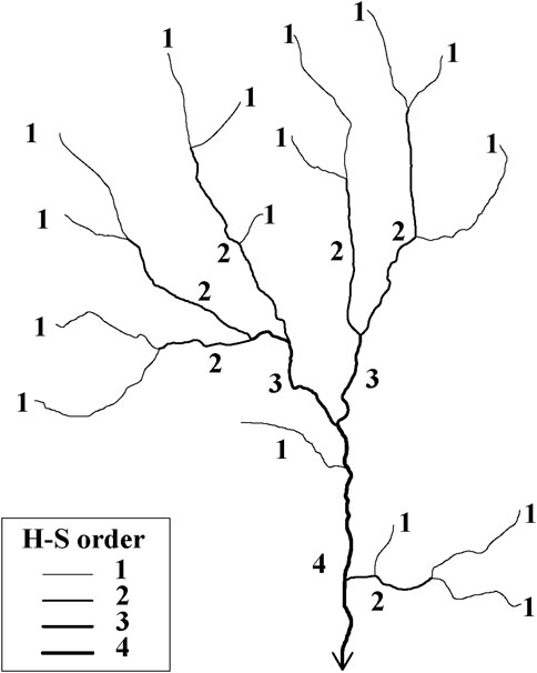
FIGURE 1. H-S ordering method schematic diagram for the illustrated river network with H-S order 4. There are 16 streams with H-S order 1, 6 streams with H-S order 2, 2 streams with H-S order 3, and 1 stream with H-S order 4. The arrow at the bottom is the outlet of this river network.
Tokunaga (1966) proposed an extended ordering method based on the H-S order. The Tokunaga ordering method reflects the topological relation of a side-branching tributary flowing into another stream with a higher order. His work plays an important role in analyzing the topology of river networks because it represents the inherent self-similarity of a river network.
A stream with H-S order
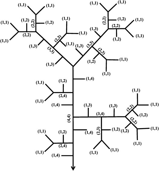
FIGURE 2. Schematic diagram for the Tokunaga ordering method for a binary tree (from Zhang et al., 2009).
For a binary tree network, the Tokunaga stream number matrix N specifies the number of streams with Tokunaga order
For example, the Tokunaga stream number matrix of the binary tree in Figure 2 is:
Eq. 2 defines the ordering method in Figure 2, which shows 22 streams with Tokunaga order (1,1), 11 streams with Tokunaga order (1,2), and so on.
The Tokunaga side-branching ratio
An upper triangular matrix T, which is calculated in terms of the Tokunaga stream number matrix N by Eq. 3, is defined as the side-branching ratio matrix with a dimension of
The necessary condition for a network to be self-similar is that the side-branching ratio
For a network to be a Tokunaga tree in a statistical sense, the side-branching ratio must satisfy the constraint (Peckham, 1995a):
Here,
In Figure 2,
Iterative Binary Tree Networks
The basic elements of a synthetic iterative network are 1) the generators, which are the smallest units of an iterative network, and 2) the iteration rules, which specify the growth pattern of the network using the generators. Different combinations of generators and iteration rules result in different networks. Iterative network models must be based on a series of generators. Each generator should be unique, and the generator series should be complete (Zhang et al., 2009; Mantilla et al., 2010).
Generator Series
Self-similarity has been considered to be an inherent characteristic of river networks since Mandelbrot first described their fractal nature (Mandelbrot, 1982; Peckham, 1995b). Since then, various methods to create synthetic networks have been proposed based on generator iteration (Veitzer and Gupta, 2000; Wang and Wang, 2002; Hung and Wang, 2005; Zhang et al., 2009; Mantilla et al., 2010). However, generators are not sequential and complete until they are cataloged by their topological structure (Zhang et al., 2009; Mantilla et al., 2010). Figure 3 shows the first four generators in a generator series. Each generator in the series can be denoted by an index λ, which is a positive integer in sequential order. The generator series in Figure 3 is the basis of the iterative networks discussed in this paper.
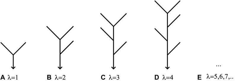
FIGURE 3. Diagrammatic infinite generator series for the topological structure of iterative binary tree networks. Here, λ is the index of each generator [revised from Zhang et al. (2009)].
Iteration Rule
The generation of a synthetic iterative network, specifically an ITBN, is based on iteration definitions and rules. First, we give some basic definitions for an iterative network. An exterior link is an unbroken section of stream that extends from a source to the first junction, and corresponds to a stream with H-S order 1, whereas an interior link connects two successive junctions or the last junction with the outlet (Shreve, 1966). The generators for the replacement of interior and exterior links are chosen from the series in Figure 3 and are denoted by λi and λo, respectively. Both interior and exterior links are replaced by the interior generator λi and exterior generator λo, respectively, in each step of the iterative process. The length of each link is assumed to be 1 in this paper. We use one link as the initial case (t = 0), and then the exterior generator λo as the first iterative step (t = 1).
The iteration rule discussed in this paper is taking λi as the constant interior generator and λo as the constant exterior generator in each step of the iterative process. This iteration rule is quasi-uniform because of the consistent generators in every iterative step. Therefore, the iterative network generated by this rule is defined as a QU-IBTN. Figure 4 shows two examples of how to generate QU-IBTNs using λi = 1, λo = 2 (Figures 4A–D) and λi = 2, λo = 3 (Figures 4E–H), respectively.
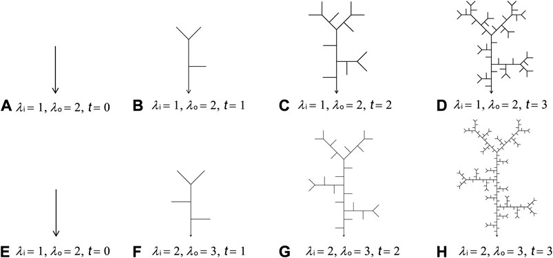
FIGURE 4. QU-IBTNs (A) and (E): initial cases (t = 0); (B–D): generator λi = 1 and λo = 2 after 1, 2, and 3 iteration steps; (F–H): generator λi = 2 and λo = 3 after 1, 2, and 3 iteration steps.
The invariance of generators in each iterative step for QU-IBTNs is strictly consistent with the definition of self-similarity. However, although the relevant iterative processes must not only have the sequentially and mathematically expressible generator series, but must also agree with the explicit given iteration rule, whether the QU-IBTN is a Tokunaga tree has never been examined graphically and recursively using a mathematical method.
Side Tributary Distribution of QU-IBTNs
The generation of a QU-IBTN begins with one link, the interior generator λi, and the exterior generator λo (i.e. the QU-IBTN is λo itself when t = 1). According to the iteration rule and Tokunaga ordering method, there are five stream number generating laws that must be obeyed during the iterative process.
The components of the generating law equations are defined as follows:
Law 1: H-S Order Law
The H-S order of the QU-IBTN is
Law 1 serves to replace the upper bound of the H-S order with the iterative step number in the calculations.
Law 2: Iteration Unchanging Law
The H-S orders of every stream and the entire network increase by 1 from the
By recursion from the
Law 2 ensures that the corresponding equality relationship between the number of streams in the different iterative steps is satisfied.
Law 3: The Source Stream Law
Every pair of source streams with order
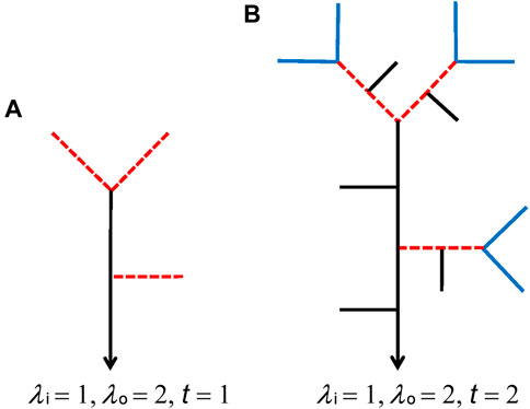
FIGURE 5. Generation of sources in the iterative process. The sources at the second step are generated by the exterior links at the first step. The red dotted lines in both (A) and (B) are the exterior links of QU-IBTNs at the first step in (A). The blue lines in (B) are the sources at the second step that are generated by the red dotted lines.
Figure 5 shows the generation of sources in Figure 5B from exterior links in Figure 5A. Consequently, the relationship between the sources at the
According to Eq. 9 in Law 2 and Eq. 10, the number of streams with order
Law 4: The Neighbor-Ordered Side-branch Law
In every iterative step, the relationship between the number of streams with Tokunaga order (1,1) and order (1,2) that depend on the exterior generator
Figure 6 shows a ratio of 3/6 for the number of streams with the order (1,2) and the number of streams with the order (1,1) in the QU-IBTN generated by the choices λi = 1, λo = 2 at the second iterative step.
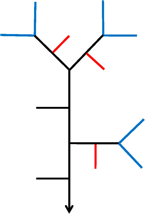
FIGURE 6. The QU-IBTN generated by λi = 1, λo = 2, t = 2 at the second step. The red lines are the streams with Tokunaga order (1,2) and the blue lines are the sources, which are the streams with Tokunaga order (1,1).
According to Eq. 9 in Law 2 and Eq. 12, the number of side branches that flow into streams that are 1 order greater (i.e.,
Law 5: The Greater-Ordered Side-branch Law
1) The streams with Tokunaga order (1,3) at the
According to Equation 9 and 14, the number of side branches that flow into streams that are 2 orders greater [i.e.,
Figure 7 shows the generation of streams with Tokunaga order (1,3) in the QU-IBTN with λi = 1, λo = 2, from the second to third iterative step.
2) The streams with Tokunaga order
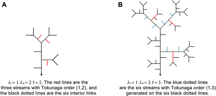
FIGURE 7. Streams with Tokunaga order (1,3) in QU-IBTNs are generated using λi = 1, λo = 2 from the second step in (A) to third iterative step in (B).
Figure 8 shows the generation of streams with Tokunaga order (1,4) in the QU-IBTN with λi = 1, λo = 2 from the second to third iterative step.
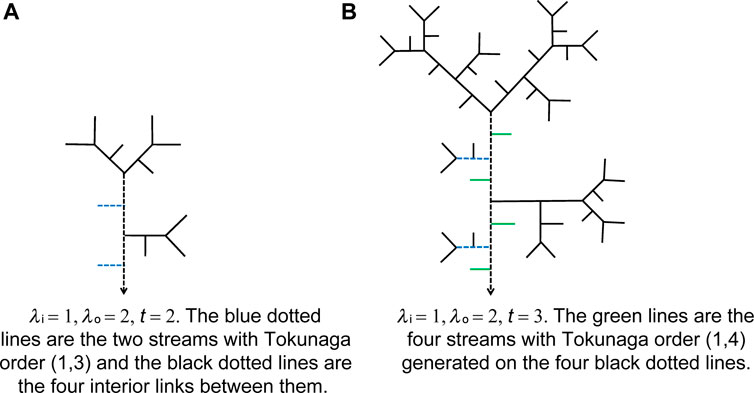
FIGURE 8. Streams with Tokunaga order (1,4) in QU-IBTNs are generated using λi = 1, λo = 2 from the second step in (A) to third iterative step in (B).
According to Equation 9 and 16, the number of side branches that flow into streams that are
Tokunaga Matrix
During the
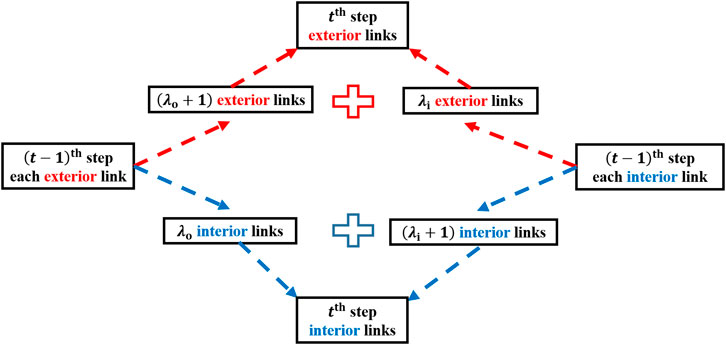
FIGURE 9. The generation of each interior and exterior link from the
Eq. 18 describes the relationship for increase of exterior and interior links between the
For the initial condition
From Eqs 10, Eqs 18, it is clear that the number of exterior links at the
The Tokunaga matrix
Using the first row of
In the following equations,
In the first column of
In the second column of
In the third column of
In the
In the
The recursion of elements in Eqs 21–25 form the matrix
The sum of the
Furthermore, the number of streams (1,1) at the
Side-Branching Ratio Matrix
The side-branching ratio matrix
We can get the expression for
We modify the form of
By combining Eq. 3 and the condition
Using Eqs 31, 32, we get the matrix
The efficient and necessary condition to be a self-similar network is that
For strict Tokunaga self-similarity, the elements in
No matter which values of
To demonstrate the constraints on self-similarity versus Tokunaga self-similarity, we provide the following two examples.
Example 1:
When the generators
The side-branching ratio
Example 2:
When the exterior link generator and the interior link generator satisfy the condition
According to Eq. 37, this QU-IBTN is a Tokunaga tree with
Results
Natural River Networks
In the following, we use the Yellow River in China (H-S order 11) and the Amazon River in South America (H-S order 12) as examples to verify whether or not they follow the rules of QU-IBTNs and the constraint of a Tokunaga tree. Figure 10 shows the river networks extracted from digital elevation model (DEM) data with a 30 m resolution (Li et al., 2018; Li et al., 2020).
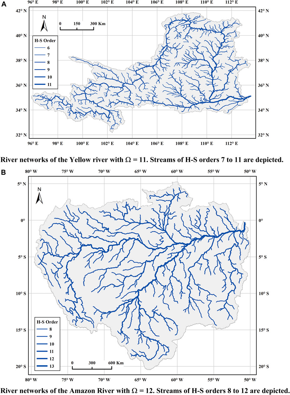
FIGURE 10. River networks of the Yellow River and the Amazon River with streams of no less than an H-S order 7 are shown in the figure.
Supplementary Table S1 (shown in Supplementary Material) shows the Tokunaga matrices of the stream numbers
The similarities Between Natural River Networks and Tokunaga Trees
Supplementary Table S2 (shown in Supplementary Material) shows the side-branching ratio matrices for the side-branching ratios
Supplementary Table S2 also shows that the branching ratio values have large fluctuations for main stems with large H-S orders, as shown in Figure 11.
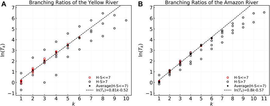
FIGURE 11. Branching ratios,
The statistical side-branching ratio matrices of the two rivers in Supplementary Table S2 and Figure 11 show that the statistical results of
The side-branching ratio series in Figure 11 were verified to satisfy as 1.34 × 2.25k−1 and 1.26 × 2.23k−1 using the least squares method, as shown in Figure 11 in terms of the dotted black lines with coefficients of determination R2 > 0.99.
Therefore, the Tokunaga parameters can be evaluated using
The Similarities Between Natural River Networks and QU-IBTNs
We construct
and
The
According to the standard form of the Tokunaga matrix
We calculate
In the
1) The exterior generators
2) The interior generators
3) The interior generators
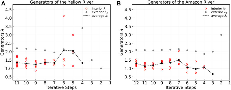
FIGURE 12. Generators of the Yellow River and the Amazon River for each iterative step. The gray solid points are the exterior generators
Table 1 lists the generators and Tokunaga parameters for the Yellow River and the Amazon River.
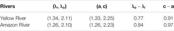
TABLE 1. The generators (
Analysis and conclusions for Table 1:
1) In our analysis, we have removed the main stems with high H-S orders at the low iterative steps, as these are controlled by the local geomorphology and terrain. The QU-IBTN rules and Tokunaga self-similarity are well demonstrated using the Yellow River and the Amazon River in terms of the uniformity and equality of the generators and branching ratios for streams with low H-S orders at high iterative steps.
2) According to the sufficient and necessary condition for a QU-IBTN to be a Tokunaga tree in Eq. 35, we should have
Discussion
The QU-IBTNs proposed above illustrate how to generate iterative binary tree networks simulating natural river networks. The complete mathematic iterative steps with graphic deduction are demonstrated in iterative orders. The iterative process is sustained by the self-similarity theory. The synthetic QU-IBTNs are close to the natural river networks in similarity characteristics parameters by two examples.
When generated by exterior generator
Although in theory the Shreve model should be the most ideal topology network that approaches natural river networks because it is a Tokunaga tree and plane-filling, there is an obvious contradiction that topological parameters such as
We have supposed that the hypothesis of the uniformity of link length in the IBTN may lead to differences in the bifurcation ratio as compared with natural river networks under the condition of plane-filling. The link length and confluence angles of IBTNs should be redefined according to the values of the stream length ratios of natural river networks when considering plane-filling.
Some aspects of the linkages between the structure of river networks and the processes that shape them remain somewhat unclear and difficult to understand (Abrahams, 1984; Montgomery and Dietrich, 1992; Perron et al., 2012; Seybold et al., 2017). A considerable body of research is available on the topologic structure associated with stream numbers and self-similarity of river networks (Peckham, 1995a; Dodds, 2000; Pelletier and Turcotte, 2000; Veitzer and Gupta, 2000; Mcconnell and Gupta, 2008; Mantilla et al., 2010; Zanardo et al., 2013). Recently, confluence angles (also referred to as junction angles) of a number of natural river networks, which represent a geometric component of river network structure, have been statistically evaluated and shown to depend on the climatic setting (Devauchelle et al., 2012; Seybold et al., 2017). These treatments of confluence angles may provide important clues in further studies to explore the following two questions: 1) where does a stream emerge from an unchannelized region? and 2) how far downstream does this stream extend until it merges into another stream?
Conclusion
In this paper we provide a complete mathematical and graphical deduction of QU-IBTNs with specified generator series and iteration rule. Our conclusions are as follows:
1) For the QU-IBTN generated by the generator series and iteration rule in this paper, five intrinsic stream number laws—which determine the distribution of source streams and side-branches following into streams of greater orders—are graphically and recursively analyzed and satisfied.
2) As defined in this paper, the QU-IBTN are demonstrated to be self-similar.
3) The sufficient and necessary constraint for a QU-IBTN to be a Tokunaga tree is that the exterior links must be replaced with a neighboring generator in the generator series that is larger than the interior links during the iterative process. This defines a generation method for a simulated network that is identical to a natural river network in topology.
4) Two natural river networks, i.e. the Yellow River, China and the Amazon River, South America, are shown to be Tokunaga trees and QU-IBTNs within specified H-S order scales.
The self-similarity of river networks is a classical topic, and there are many researchers working on this topic using varied methods, including mathematicians who are good at fractal theory (Kovchegov and Zaliapin, 2020). Other researchers might use random and mathematical foundations in their own research. Our manuscript here is an intuitive, accessible and understandable initial tool to measure the self-similarity of river networks. The advance of generator series, the integer iterative rules showing directly by graphs, and the corresponding mathematical derivations are new and different from others’ methods. The QU-IBTNs are built just in a few finite iterative steps as shown in the figures. QU-IBTNs in random scales will be generated by coding in the future. However, to some extent we are doing the same thing as other researchers-just find a way to demonstrate the self-similarity and Tokunaga property of river networks. This is what we think we can share with other researchers, and help make progress in river network simulations in the future.
Methods
The Method for Calculating
For the
The interior generators in the
and
In the matrix
For the Yellow River and the Amazon River, the statistically averaged values for
and
For the Yellow River and the Amazon River, the statistically averaged values for
and
Data Availability Statement
The original contributions presented in the study are included in the article/Supplementary Material, further inquiries can be directed to the corresponding author.
Author Contributions
LZ, the corresponding author, did all the mathematics derivations. KYW organized the manuscript. TJL did the derivations and provided the data. XL, BYG, and GXC collected the data and plot figures. JHW and YFH processed the data and revised the manuscript.
Funding
This paper is supported by the State Key laboratory of Plateau Ecology and Agriculture, Qinghai Univerisity (2021-KF-10), National Natural Science Foundation of China (52109092), and Huazhong University of Science and Technology (3004242101).
Conflict of Interest
The authors declare that the research was conducted in the absence of any commercial or financial relationships that could be construed as a potential conflict of interest.
Publisher’s Note
All claims expressed in this article are solely those of the authors and do not necessarily represent those of their affiliated organizations, or those of the publisher, the editors and the reviewers. Any product that may be evaluated in this article, or claim that may be made by its manufacturer, is not guaranteed or endorsed by the publisher.
Acknowledgments
Data supporting Figure 10 and Supplementary Table S1 in this study were obtained from a digital elevation model (DEM) data with a 30 m resolution. I would like to thank Rina Schumer and Gary Parker for their useful comments and revisions of the manuscript.
Supplementary Material
The Supplementary Material for this article can be found online at: https://www.frontiersin.org/articles/10.3389/fenvs.2021.792289/full#supplementary-material
Supplementary Table S1 | The Tokunaga matrices
Supplementary Table S2 | The side-branching ratio matrices
Supplementary Table S3 | The
Supplementary Table S4 | The
References
Abrahams, A. D. (1984). The Development of Tributaries of Different Sizes along Winding Streams and Valleys. Water Resour. Res. 20, 1791–1796. doi:10.1029/wr020i012p01791
Claps, P., Fiorentino, M., and Oliveto, G. (1996). Informational Entropy of Fractal River Networks. J. Hydrol. 187, 145–156. doi:10.1016/s0022-1694(96)03092-2
Devauchelle, O., Petroff, A. P., Seybold, H. F., and Rothman, D. H. (2012). Ramification of Stream Networks. Proc. Natl. Acad. Sci. 109, 20832–20836. doi:10.1073/pnas.1215218109
Dodds, P. S. (2000). Geometry of River Networks. Ph.D. Thesis. Massachusetts Institute of Technology.
Dodds, P. S., and Rothman, D. H. (1999). Unified View of Scaling Laws for River Networks. Phys. Rev. E 59, 4865–4877. doi:10.1103/PhysRevE.59.4865
Gupta, V. K., and Mesa, O. J. (2014). Horton Laws for Hydraulic-Geometric Variables and Their Scaling Exponents in Self-Similar Tokunaga River Networks. Nonlin. Process. Geophys. 21, 1007–1025. doi:10.5194/npg-21-1007-2014
Horton, R. E. (1945). Erosional Development of Streams and Their Drainage Basins; Hydrophysical Approach to Quantitative Morphology. Geol. Soc. Am. Bull. 56 (3), 275–370. doi:10.1130/0016-7606(1945)56[275:edosat]2.0.co;2
Hung, C.-P., and Wang, R.-Y. (2005). Coding and Distance Calculating of Separately Random Fractals and Application to Generating River Networks. Fractals 13 (1), 57–71. doi:10.1142/S0218348X05002738
Kovchegov, Y., and Zaliapin, I. (2020). Random Self-Similar Trees: A Mathematical Theory of Horton Laws. Probab. Surv. 17, 1–213. doi:10.1214/19-PS331
Li, J., Li, T., Liu, S., Shi, H., and Shi, H. Y. (2018). An Efficient Method for Mapping High-Resolution Global River Discharge Based on the Algorithms of Drainage Network Extraction. Water 10 (4), 533. doi:10.3390/w10040533
Li, J. Y., Li, T. J., Zhang, L., Bellie, S., Fu, X. D., Huang, Y. F., et al. (2020). A D8-Compatible High-Efficient Channel Head Recognition Method. Environ. Model. Softw. 125, 104624. doi:10.1016/j.envsoft.2020.104624
Mantilla, R., Troutman, B. M., and Gupta, V. K. (2010). Testing Statistical Self-Similarity in the Topology of River Networks. J. Geophys. Res. 115, 1–12. doi:10.1029/2009JF001609
Masek, J. G., and Turcotte, D. L. (1993). A Diffusion-Limited Aggregation Model for the Evolution of Drainage Networks. Earth Planet. Sci. Lett. 119, 379–386. doi:10.1016/0012-821x(93)90145-y
Mcconnell, M., and Gupta, V. K. (2008). A Proof of the Horton Law of Stream Numbers for the Tokunaga Model of River Networks. Fractals 16 (3), 227–233. doi:10.1142/S0218348X08003958
Menabde, M., Veitzer, S., Gupta, V., and Sivapalan, M. (2001). Tests of Peak Flow Scaling in Simulated Self-Similar River Networks. Adv. Water Resour. 24, 991–999. doi:10.1016/S0309-1708(01)00043-4
Montgomery, D. R., and Dietrich, W. E. (1992). Channel Initiation and the Problem of Landscape Scale. Science 255, 826–830. doi:10.1126/science.255.5046.826
Peckham, S. D. (1995b). Self-similarity in the Three-Dimensional Geometry and Dynamics of Large River Basins. Ph.D.Thesis. USA: University of Colorado.
Peckham, S. D. (1995a). New Results for Self-Similar Trees with Applications to River Networks. Water Resour. Res. 31 (4), 1023–1029. doi:10.1029/94WR03155
Pelletier, J. D., and Turcotte, D. L. (2000). Shapes of River Networks and Leaves: Are They Statistically Similar? Phil. Trans. R. Soc. Lond. B 355, 307–311. doi:10.1098/rstb.2000.0566
Perron, J. T., Richardson, P. W., Ferrier, K. L., and Lapôtre, M. (2012). The Root of Branching River Networks. Nature 492, 100–103. doi:10.1038/nature11672
Seybold, H., Rothman, D. H., and Kirchner, J. W. (2017). Climate's Watermark in the Geometry of Stream Networks. Geophys. Res. Lett. 44 (5), 2272–2280. doi:10.1002/2016gl072089
Strahler, A. N. (1952). Hypsometric (Area-altitude) Analysis of Erosional Topography. Geol. Soc. Am. Bull. 63, 1117–1142. doi:10.1130/0016-7606(1952)63[1117:haaoet]2.0.co;2
Tokunaga, E. (1978). Consideration on the Composition of Drainage Networks and Their Evolution, Geograph. Rep 13, 1–27.
Tokunaga, E. (1984). Ordering of divide Segments and Law of divide Segment Numbers. Trans. Jpn. Geomorphol. Union 5 (2), 71–77.
Tokunaga, E. (1966). The Composition of Drainage Network in Toyohira River basin and Valuation of Horton’s First Law (In Japanese with English Summary). Geophys. Bull. Hokkaido Univ. 15, 1–19.
Troutman, B. M. (2005). Scaling of Flow Distance in Random Self-Similar Channel Networks. Fractals 13, 265–282. doi:10.1142/S0218348X05002945
Veitzer, S. A., and Gupta, V. K. (2000). Random Self-Similar River Networks and Derivations of Generalized Horton Laws in Terms of Statistical Simple Scaling. Water Resour. Res. 36 (4), 1033–1048. doi:10.1029/1999WR900327
Veitzer, S. A., and Gupta, V. K. (2001). Statistical Self-Similarity of Width Function Maxima with Implications to Floods. Adv. Water Resour. 24, 955–965. doi:10.1016/S0309-1708(01)00030-6
Wang, G. Q., Li, T. J., Zhang, L., et al. (2016). River basin Geometry. Beijing, China: Science Press, 133–138. (in Chinese).
Wang, P.-J., and Wang, R.-Y. (2002). A Generalized Width Function of Fractal River Network for the Calculation of Hydrologic Responses. Fractals 10 (2), 157–171. doi:10.1142/S0218348X02001038
Zanardo, S., Zaliapin, I., and Foufoula-Georgiou, E. (2013). Are American Rivers Tokunaga Self-Similar? New Results on Fluvial Network Topology and its Climatic Dependence. J. Geophys. Res. Earth Surf. 118, 1–18. doi:10.1002/jgrf.2002910.1029/2012jf002392
Zhang, L., Dai, B., Wang, G., Li, T., and Wang, H. (2009). The Quantization of River Network Morphology Based on the Tokunaga Network. Sci. China Ser. D-Earth Sci. 52 (11), 1724–1731. doi:10.1007/s11430-009-0176-y
Glossary
N Tokunaga stream number matrix composed by
T Tokunaga side-branching ratio matrix composed by
Keywords: horton-strahler (H-S) order, tokunaga tree, generator series, side tributary distribution, self-similarity, iterative binary tree network
Citation: Wang K, Zhang L, Li T, Li X, Guo B, Chen G, Huang Y and Wei J (2022) Side Tributary Distribution of Quasi-Uniform Iterative Binary Tree Networks for River Networks. Front. Environ. Sci. 9:792289. doi: 10.3389/fenvs.2021.792289
Received: 10 October 2021; Accepted: 12 November 2021;
Published: 03 January 2022.
Edited by:
Jaan H. Pu, University of Bradford, United KingdomReviewed by:
Haiyun Shi, Southern University of Science and Technology, ChinaSongdong Shao, Dongguan University of Technology, China
Copyright © 2022 Wang, Zhang, Li, Li, Guo, Chen, Huang and Wei. This is an open-access article distributed under the terms of the Creative Commons Attribution License (CC BY). The use, distribution or reproduction in other forums is permitted, provided the original author(s) and the copyright owner(s) are credited and that the original publication in this journal is cited, in accordance with accepted academic practice. No use, distribution or reproduction is permitted which does not comply with these terms.
*Correspondence: Li Zhang, bGl6aGFuZ3BpZ0BnbWFpbC5jb20=