Estimation of Surface and Near-Surface Air Temperatures in Arid Northwest China Using Landsat Satellite Images

Near-surface air (Ta) and land surface (Ts) temperatures are essential parameters for research in the fields of agriculture, hydrology, and ecological changes, which require accurate datasets with different temporal and spatial resolutions. However, the sparse spatial distribution of meteorological stations in Northwest China may not effectively provide high-precision Ta data. And it is not clear whether it is necessary to improve the accuracy of Ts which has the most influence on Ta. In response to this situation, the main objective of this study is to estimate Ta for Northwest China using multiple linear regression models (MLR) and random forest (RF) algorithms, based on Landsat 8 images and auxiliary data collected from 2014 to 2019. Ts, NDVI (Normalized Difference Vegetation Index), surface albedo, elevation, wind speed, and Julian day were variables to be selected, then used to estimate the daily average Ta after analysis and adjustment. Also, the Radiative Transfer Equation (RTE) method for calculating Ts would be corrected by NDVI (RTE-NDVI). The results show that: 1) The accuracy of the surface temperature (Ts) was improved by using RTE-NDVI; 2) Both MLR and RF models are suitable for estimating Ta in areas with few meteorological stations; 3) Analyzing the temporal and spatial distribution of errors, it is found that the MLR model performs well in spring and summer, and is lower in autumn, and the accuracy is higher in plain areas away from mountains than in mountainous areas and nearby areas. This study shows that through appropriate selection and combination of variables, the accuracy of estimating the pixel-scale Ta from satellite remote sensing data can be improved in the area that has less meteorological data.

Introduction

Near-surface air temperature (Ta), usually refers to the air temperature at 2 m above the ground, is an essential factor affecting ecology, agriculture, and urban areas (Raja Reddy et al., 1997; Krüger and Emmanuel, 2013; Shamir and Georgakakos, 2014), and is also the basis for climate change studies (Alkama and Cescatti, 2016; Bathiany et al., 2018). The traditional method of obtaining Ta mainly relies on the temperature sensor installed at the meteorological station, and the interpolation method is frequently used to extend to regional-scale applications (Mostovoy et al., 2006). If the meteorological stations are sparse and unevenly distributed, the accuracy of the interpolation method will be greatly restricted due to the influence of underlying surface heterogeneity and heat conduction unevenness to air temperature (Chen et al., 2015). The air temperature has become the primary driving variable of many land surface models (Nieto et al., 2011), so its spatial fidelity must be higher than that obtained by interpolation of point observation data, and even the most complex geostatistical techniques cannot meet the requirements (Prince et al., 1998).

Satellite data has the characteristics of continuous spatial coverage (Czajkowski et al., 1997), which can obtain large-scale atmospheric information and invert surface parameters, including global surface temperature, vegetation index, elevation, and other information (Wang et al., 2018; Yoo et al., 2018). Due to the complexity of atmospheric radiation and its low proportion in remote sensing signals, Ta cannot be directly reversed (Xu et al., 2012; Li and Zha, 2018). However, Ta can be obtained by establishing the regression relationship between Ta and remote sensing inversion and auxiliary parameters, such as using land surface temperature (Ts), Normalized Difference Vegetation Index (NDVI), wind speed, geographic location and elevation, among which Ts is the most important parameter (Vancutsem et al., 2010; Hachem et al., 2012; Song and Wu, 2018).

Ts as the direct driving force of long-wave radiation and turbulent heat flux exchange at the surface-atmosphere interface is one of the most significant parameters in the physical process of surface energy and water balance at regional and global scales (Anderson et al., 2008; Li et al., 2013; Orhan et al., 2014; Folland et al., 2018). At present, there are three main methods for using Landsat to retrieve Ts: atmospheric correction method (also known as Radiative Transfer Equation: RTE), Single Channel Algorithm (SCA), and Split Window Algorithm (SWA). The SWA does not require any atmospheric profile information at the time of collection, which needs to use two thermal infrared channels (Li et al., 2013). However, the United States Geological Survey has pointed out that Thermal Infrared Sensor (TIRS) 11th band has data reception abnormalities and calibration instability problems, which mainly affects the accuracy of the split window algorithm applied to Landsat-8 TIRS data to retrieve Ts (Xu, 2015). SCA and RTE rely on atmospheric transmissivity and upwelling and downwelling atmospheric radiances (Jimenez-Munoz et al., 2009; Sekertekin and Bonafoni, 2020). RTE removes the error caused by the atmosphere’s thermal radiation on the surface and converts the thermal radiation intensity to the corresponding Ts (Ma and Pu, 2020). When using different data sets, the performance of the RTE method to retrieve Ts is also different. The Ts calculation result for Landsat TM 5 data is better than other methods in the same period with RMSE is 1–3°C (Sobrino et al., 2004; Ndossi and Avdan, 2016; Windahl and Beurs, 2016); however, the RMSE calculated based on Landsat 8 TIRS 10th band was 1.5–5°C, and most of them are inferior to other algorithms (Ndossi and Avdan, 2016; Wang et al., 2016; Sekertekin and Bonafoni, 2020). Moreover, the overestimation shown in the TIRS band will increase as the proportion of vegetation decreases (Xu and Huang, 2016).

Several studies have used surface information to estimate air temperatures, such as the temperature-vegetation index (TVX), energy balance, statistics, and machine learning methods (Zakšek and Schroedter-Homscheidt, 2009; Benali et al., 2012). Nemani and Running (1989), Goward et al. (1994) proposed the TVX approach to estimate near surface air temperature with promising results. The method is based on the assumption that there is a strong negative correlation between Ts and vegetation index (Goward et al., 1994; Czajkowski et al., 1997). Assuming that the Ta for fully covered vegetation is close to Ts, the value of full coverage NDVI (NDVImax) can be used to obtain an approximate value of Ta (Stisen et al., 2007; Nieto et al., 2011; Zhu et al., 2013). However, this assumption does not apply to all seasons, soil moisture, and ecosystem types, so estimation of Ta by using TVX method is not feasible in areas or seasons without high vegetation cover (Vancutsem et al., 2010).

The energy balance method has a physical mechanism, so it has well portability and versatility (Hou et al., 2013; Shen et al., 2020). According to the energy balance equation, Ta is related to surface temperature, and it depends on various environmental factors such as solar radiation, cloud cover, wind speed, soil moisture, and surface type (Prince et al., 1998). A large number of required parameters cannot be completely retrieved by remote sensing (Mostovoy et al., 2006), so it is difficult to use remote sensing to perform Ta inversion in the area. The issue of unclosed surface energy balance also brings additional uncertainty to this method (Zhang et al., 2015).

Statistical methods need to analyze the relationship between Ta and Ts and other auxiliary data, and then build an estimation model based on specific correlation (Cresswell et al., 1999; Park, 2011), which including simple statistical models, multiple linear regression (MLR) models, geographically weighted regression (GWR) models, and machine learning methods (Vogt et al., 1997; Vancutsem et al., 2010; Shen et al., 2020). Studies have shown that the linear regression models are more accurate in calculating the average daily temperature with a root mean square error (RMSE) ranging between 1.29–3.60°C (Chen et al., 2015; Shi et al., 2016; Yang et al., 2017), which can produce good results in a specific space and time range, but require a large amount of data involved in the calculation and training of the algorithms (Stisen et al., 2007). Geographically weighted statistical and machine learning methods usually have higher accuracy (Moser et al., 2015; Wang et al., 2017, 2018). Geographically and temporally weighted regression (GTWR) is an extension of the general linear regression model, which embeds changes in location and time into the regression equation and estimates regression coefficients for spatio-temporal variation by performing local regressions that can solve for constant-coefficient limits (Bai et al., 2016; Li et al., 2018). Machine learning methods can handle non-linear and highly correlated predictors (James et al., 2013) and estimate the temperature in areas with complex and heterogeneous underlying surfaces, mainly including neural networks (Jang et al., 2004), M5 model trees (Emamifar et al., 2013), and random forests (Zhang et al., 2016), support vector machine (Moser et al., 2015). Random forests (RF) are widely used and have been verified in various terrains. Ho et al. (2014) indicated that the RF algorithm is very useful for mapping the variability of urban internal temperature. Meyer et al. (2016) have pointed out that compared with linear regression, generalized augmented regression model (GBM), and cubic regression, the RF algorithm performs poorly in the extremely cold Antarctica. However, Noi et al. (2017) have shown reliable results in mountainous areas. Therefore, the conclusion of RF estimation Ta still needs to be discussed.

Most of the current researches for estimating Ta is based on the MODIS due to its time continuity advantage, but its resolution cannot meet the demand for farmland or even smaller scales. The spatial resolution of Landsat 8 imagery is higher than that of MODIS, and the estimated Ta data have a more intuitive correspondence with land use. Generally, if the temperature estimate based on remote sensing data is accurate, the accuracy should be between 1 and 2°C (Vázquez et al., 1997). Research suggests that site density is positively correlated with model accuracy. In other words, the denser the sites, the higher the accuracy of the model (Shen et al., 2020). If Ta is estimated jointly in Northwest China, where meteorological stations are scarce, and in areas where other stations are d ense, the former regions often do not obtain more accurate Ta data (Chen et al., 2015; Li and Zha, 2018). Therefore, it is very necessary to separately model and estimate the area where the data is lacking.

The main objective of this study was to propose a statistical method based on Landsat 8 and auxiliary data for accurately estimating Ta, especially in arid northwest China, where meteorological stations are scarce and unevenly distributed. The specific objectives of this study were to 1) use the RTE method to estimate Ts based on the Landsat8 data, and improve accuracy. 2) Select reasonable independent variables, participate in the modeling of MLR and RF, and compare the results of Ta estimation. 3) Evaluate the performance of the optimal Ta estimation model in time and space scale.

Materials and Methodology

Study Region and Meteorological Station

The study area is the Shiyang River basin in the arid region of Northwest China, which is located in the Hexi Corridor of Gansu Province and the coordinate range is between 101°40′E-104°20′E and 36°30′N-39°30′ N (Figure 1). It covers an area of 41,600 km², and the range of altitude is 1,157m–5012 m. This area is of a continental temperate arid climate, with the characteristics of aridity where precipitation is 300 mm per year and average annual pan evaporation is 2,000 mm.

FIGURE 1

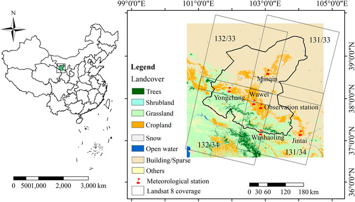
FIGURE 1. The location of the study area, the coverage area of Landsat8, distribution of meteorological stations, and land use cover.

Meteorological stations in Northwest China are sparse, with only five stations in and near the study area (Minqin, Wuwei, Yongchang, Wushaoling, Jintai station), which can be collected from the China Meteorological Science Data Center (http://data.cma.cn). The observation station (National Field Scientific Observation and Research Station on Efficient Water Use of Oasis Agriculture in Wuwei of Gansu Province) has a meteorological station to collect Ta data, SI-111 thermal infrared radiometers to obtain Ts data (the coordinates in Table 1). Google Earth Pro was used to verify the location of the meteorological station and ensure that Ta data corresponds totally to the site location. Then obtain the available satellite images from 2014 to 2019 and calculate and extract the Ts data corresponding to the location of the meteorological station through the GEE platform.

TABLE 1

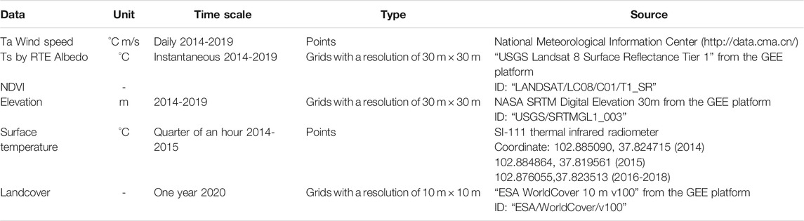
TABLE 1. Type and source of data used.

Satellite Data and Processing

Google Earth Engine (GEE) is a geospatial processing platform based on cloud computing developed by Google, which promotes fast analysis by using Google’s computing infrastructure and providing a convenient platform for applications based on linking to the cloud computing engine (Becker et al., 2021). Most of the algorithms built into the GEE cloud computing platform use pixel-by-pixel calculation functions, so no matter what the area or proportion of the calculation and analysis is required, as long as the research area has available data. The platform is suitable for scientific researchers with a background in non-professional programming and can quickly realize global-scale remote sensing data processing and mining. This research uses the online JavaScript API of the GEE platform (https://earthengine.google.com/) to access and analyze the data sets used from the public catalog, without downloading images, only outputting the processing results, which improves computing efficiency.

This study uses the Landsat 8 Raw and SR (Surface Reflectance product) dataset in the GEE platform, screening the images with cloudiness not exceeding 30% from 2014 to 2019 and perform cloud removal processing. To cover the entire area of the Shiyang River basin using images of four Landsat-8 tiles 131/033,131/034 and 132/033,132/034 (Figure 1). By using the GEE platform, the remote sensing images were spliced efficiently, clipped, and parameter inversion, also the meteorological data were interpolated.

Land Surface Temperature

At present, there are three main methods for remote sensing to retrieve land surface temperature: atmospheric Radiative Transfer Equation (RTE) method, single-channel algorithm, and split-window algorithm. This study uses the Landsat 8 SR data set in the GEE platform, to retrieve the Ts based on the RTE method.

The expression of the radiation transfer equation of the thermal infrared radiation value (L_λ) received by the satellite sensor is (Li et al., 2013; Windahl and Beurs, 2016):

$\begin{array}{c}{L}_{\text{λ}}=\left[\epsilon B\left(T_s\right)+\left(1-\epsilon \right)L\downarrow \right]\tau +L\uparrow \end{array}(1)$

where $L_{\text{λ}}$ is the spectral radiance value at the top of the atmosphere at the band λ ($W\cdot m^{-2}\cdot \mu m^{-1}\cdot s{r}^{-1}$); ε is the surface specific emissivity; B (T_s) is the blackbody thermal emissivity brightness ($W\cdot m^{-2}\cdot \mu m^{-1}\cdot s{r}^{-1}$); τ is the atmospheric thermal infrared band transmittance; L↓ is the downward radiance of the atmosphere after reflection on the ground ($W\cdot m^{-2}\cdot \mu m^{-1}\cdot s{r}^{-1}$); L↑ is the upward radiance of the atmosphere ($W\cdot m^{-2}\cdot \mu m^{-1}\cdot s{r}^{-1}$).

Knowledge of land surface emissivity (LSE) is necessary to apply the above methods to a Landsat image. Considering different situations, obtain the emissivity value from NDVI (Sobrino et al., 2004; Orhan and Yakar, 2016):

$\begin{array}{c}\epsilon =\{\begin{array}{c}0.986 \text{NDVI}\le {\text{NDVI}}_{Soil}\\ 0.004\left[\frac{\text{NDVI}-{\text{NDVI}}_{Soil}}{{\text{NDVI}}_{Veg}-{\text{NDVI}}_{Soil}}\right]+0.986{\text{NDVI}}_{Soil}<NDVI<{\text{NDVI}}_{Veg}\\ 0.990 \text{NDVI}\ge {\text{NDVI}}_{Veg}\end{array}\end{array}(2)$

where ${\text{NDVI}}_{Veg}=0.7$ and ${\text{NDVI}}_{Soil}=0.05$ (Ma and Pu, 2020).

When using Landsat8 images, take the 10th band to provide the thermal infrared radiance value. The calculation formula of $B\left(T_s\right)$ is:

$\begin{array}{c}B\left(T_s\right)=\frac{\left[L_{\text{λ}}-L\uparrow -\left(1-\epsilon \right)\tau L\downarrow \right]}{\tau \epsilon }\end{array}(3)$

The calculation of the surface temperature (T_s) uses the Planck formula:

$\begin{array}{c}{T}_s=\frac{K_2}{\ln \left(\frac{K_1}{B\left(T_s\right)}+1\right)}-273.15\end{array}(4)$

where Ts is surface temperature (°C); $K_1$, $K_2$ can be obtained from the header file of the remote sensing data. For Landsat8 TIRS Band10, $K_1=774.89W·m^{-2}\cdot \mu m^{-1}\cdot s{r}^{-1}$, $K_2=1321.08K$.

It can be seen that the use of Radiative Transfer Equation method to retrieve the Ts needs to have the atmospheric profile parameters, which can be obtained by entering the shadowing time, latitude, and longitude in the website provided by NASA (http://atmcorr.gsfc.nasa.gov/).

Auxiliary Data and Processing Flow

The near-surface air temperature (Ta) has a good correlation with the surface temperature (Ts) (Benali et al., 2012; Ruiz-Álvarez et al., 2019). Ts is a physical quantity that reflects the degree of cold and heat on the surface of a ground object because it is affected by the characteristics of the underlying surface, such as vegetation coverage and dry and wet conditions. Ta is a physical quantity reflecting the degree of cold and hot air in the atmosphere. The atmosphere has strong fluidity, which is easily affected by the surrounding environment (Xu et al., 2012; Gholamnia et al., 2017). Therefore, when looking for the correlation between Ts and Ta, the influence of various factors such as ground characteristic and environment must be considered. For the estimation of Ta, Jang et al. (2004) showed that Julian day is a more significant parameter than altitude or the solar zenith angle. In addition, we have chosen variables that are often selected as predictors in air temperature modeling literature, such as surface albedo, elevation (DEM), normalized vegetation index (NDVI), and wind speed (Riddering and Queen, 2006; Cristóbal et al., 2008; Hou et al., 2013). The full name of the DEM (WGS84/EGM96) data source is “NASA SRTM Digital Elevation 30 m,” which is used directly on the GEE platform and provided by NASA JPL (Farr et al., 2007).

The broadband albedo ($\text{α}$) of the ground surface is a critical variable for many scientific applications, which is the ratio of the total radiant flux reflected by the ground surface to the incident flux (Liang et al., 2003). The calculation formula of $\text{α}$ is:

$\begin{array}{c}\alpha =0.356{\text{α}}_2+0.130{\text{α}}_4+0.373{\text{α}}_5+0.085{\text{α}}_6+0.072{\text{α}}_7-0.0018\end{array}(5)$

Where α is the surface reflectance, and its value is between 0–1.0; α₂, α₄, α₅, α₆, and α₇ are the 2, 4, 5, 6, and 7 bands of Landsat 8 surface reflectance products.

As has been commented in the previous section, the LSE can be retrieved from NDVI values. The data can be used to construct NDVI according to the following equation:

$\begin{array}{c}NDVI=\frac{NIR-R}{NIR+R}\end{array}(6)$

Where NIR and R are the reflection values of the near-infrared and infrared bands, respectively, which are the fifth and fourth bands of Landsat 8.

This study mainly considers the relationship between Ta and Ts, NDVI, surface albedo, DEM, wind speed and Julian day. The flow chart of the models used is shown in Figure 2, and the process can be summarized as Data preparation, processing and prediction. Data collection is the basis for establishing a reliable model, but it is also necessary to filter the input variables and try to use as few variables as possible under the condition of high model accuracy. Variables used in this study are readily available, which are closely related to the changes of Ta. Previous studies on Ta estimation lack the verification of Ts and analysis of related results. Therefore, this research explored whether it is necessary to improve the precision of Ts to achieve better results in actual application. After verification and comparison, the best model is selected from the combined methods to estimate Ta.

FIGURE 2

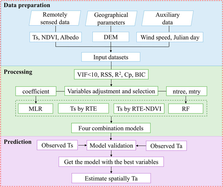
FIGURE 2. The flow chart for estimating daily mean air temperature (Ta). Input variables include surface temperature (Ts), normalized vegetation index (NDVI), surface albedo (Albedo), elevation (DEM), wind speed, and Julian day, and build MLR and RF models. Variables are selected by indicators such as variance inflation factor (VIF), residual sum of squares (RSS), coefficient of determination ( R²), Mallows Cp (Cp) value, and Bayesian Information Criterion (BIC). Finally, compare the simulation results of the four combined models with the measured values, then obtaining the Ta distribution in the study area.

The spatial and temporal matching among the variables is the main issue for the reliability of the regression implementation. Table 1 shows the sources and resolutions of all data sets. On the spatial scale, the resolutions of spatial variability independent variables such as Ts, Albedo, NDVI, elevation, wind speed (resampled after interpolation) are all 30 m × 30 m, which is spatially consistent. On the time scale, Ts, Albedo, and NDVI are instantaneous data, and only wind speed is daily data.

Models Adjustment and Validation

Multiple Linear Regression

The regression model aims to establish the corresponding functional relationship between several independent input parameters and output targets (Giacomino et al., 2011; Agha and Alnahhal, 2012; Williams and Ojuri, 2021). MLR is a linear regression technique and very useful for the best relationship between predictor variables and several independent variables, which is different from a simple linear regression analysis (Akan et al., 2015). R is an excellent tool for statistical calculation and statistical mapping. It is free, open-source software that does not require any license and is simple to operate (Williams and Ojuri, 2021). Using the “lm” function in R software, an MLR model of Ta and multiple correlation factors are established Expanding the MLR equation into the more commonly used form is:

$\begin{array}{c}A= {\text{b}}_0+ {\text{b}}_1{\text{X}}_1+{\text{ b}}_2{\text{X}}_2+ {\text{b}}_3{\text{X}}_3+\dots + {\text{ b}}_n{\text{X}}_{\text{n}}\end{array}(7)$

where A is the regression target variable; b₀∼b_n are undetermined coefficients; X₁∼X_n are independent variables.

Random Forest

The random forest (RF) is a non-parametric machine learning algorithm, which is more flexible than classical statistical models (Genuer et al., 2017; Li et al., 2019). It hardly requires statistical assumptions and is more tolerant of missing values and outliers. Due to the Law of Large Numbers, RF does not overfit. Injecting the correct randomness makes them accurate classifiers and regressors. RF algorithm can automatically distinguish the importance of each variable, give out the dependence between variables, and easily give explanations in combination with professional knowledge (Breiman, 2001). The RF method has been widely used for classification and regression in remote sensing applications (Ke et al., 2016; Park et al., 2016, 2018; Richardson et al., 2017). RF has begun to be used for Ta estimation in recent years (Ho et al., 2014; Zhang et al., 2016; Yoo et al., 2018). Use the default model parameter settings of R and its contribution packages to develop and apply statistical models (R Core Development Team, 2008; Ho et al., 2014; Liaw and Wiener, 2015).

Variable Adjustment

The absence of complete collinearity between any two independent variables is one of the assumptions of multiple linear regression. Variance Inflation Factor (VIF) is an index used to judge whether there is collinearity. If there is no linear relationship between the independent variables, the VIF value is 1, and a deviation from 1 indicates a trend of collinearity. From the effect of the multicollinearity test, multicollinearity can be tolerated when VIF <10. The VIF value of a variable greater than 10 indicates that there may be estimation problems. If there is multicollinearity, we would simply delete the variable directly, or use a biased estimate for processing (Shabani and Norouzi, 2015; Williams and Ojuri, 2021).

The Ta peaks around the 200th day of each year, which is nonlinear with the increase of Julian Day, so assuming that there is a quadratic function relationship. Linearize the Julian Day and adjust it to $x7={(J-200)}^2$ as the independent variable. The Ts and the Julian day are independent variables with a strong correlation. Therefore, adding the relationship of $x8=x7\times Ts$ as an interaction term to match the model, assuming that the slope of Ts depends on the value of Julian day.

Selecting appropriate variables can not only avoid overfitting but also increase the explanatory degree of the model. The idea of the optimal subset selection method is to model all the variable combinations, then select the model with the best result. The advantage of this method is that all possible combinations are tested, and the final choice must be the best result. However, as the number of candidate variables increases, the amount of calculation will increase exponentially. Therefore, this method is only suitable for situations with few independent variables.

Residual Sum of Squares (RSS), adjusted coefficients of determination (adjusted R²), Mallows’s Cp (Cp) value, and Bayesian Information Criterion (BIC) value are used to evaluate model statistics (Cristóbal et al., 2008). The closer Adjusted R² is to 1, and the other indicators are smaller, the better the model fits. The optimal model can be determined by comparing the indicators of each variable.

Validation Data and Indicators

The verification of Ts used the infrared sensor (SI-111) observation data in the uniform and widespread farmland from 2014 to 2018. Ta and wind speed data records for 2014–2019 come from the daily data set of surface climate data, obtaining from the China Meteorological Data Service Centre (http://data.cma.cn/). Use Ts and other independent variables from 2014 to 2017 as a training set to build the MLR model and use data from 2018 to 2019 to verify the accuracy. The RF model randomly extracts 70% of all the data as a training set, using the remaining data to validate the resulting model. Such a verification method can explore whether the model constructed by the data from the past years is also applicable to the future years, which achieve the expansion of the time scale.

A set of statistical parameters were calculated to assess the accuracy of the predicted air temperature, including coefficients of determination (R²), root mean square error (RMSE), and model efficiency (MEF). Values of R², RMSE, MEF and can be estimated using the following equations:

$\begin{array}{c}{\text{R}}^2=\frac{{{\displaystyle \sum }}_{i=1}^n\left[\left(y_i-\overline{y}\right)\left(O_i-\overline{O}\right)\right]}{{{\displaystyle \sum }}_{i=1}^n\left[{\left(y_i-\overline{y}\right)}^2\right]{{\displaystyle \sum }}_{i=1}^n\left[{\left(O_i-\overline{O}\right)}^2\right]} \end{array}(8)$

$\begin{array}{c}\text{RMSE}= {\left[{\displaystyle \sum }_{i=1}^n\frac{{\left(O_i-y_i\right)}^2}{n}\right]}^{\raisebox{1ex}{$1$}\!\left/ \!\raisebox{-1ex}{$2$}\right.}\end{array}(9)$

$\begin{array}{c}\text{MEF}=1-\left({\displaystyle \sum }_{i=1}^n\frac{{\left(O_i-y_i\right)}^2}{\sum _{i=1}^n{\left(O_i-\overline{O}\right)}^2}\right)\end{array}(10)$

where n is the number of records in validation data sets used in this study, $y_i$ is the estimated variable, and $O_i$ is the observed variable, $\overline{y}$ is the mean value of the predicted for all validation sites, $\overline{O}$ is the mean value of the observed variable for all validation sites.

R² always calculated for a significance level of 0.005, was used as a measure of correlation and proportion of observed variability accounted by the model (Benali et al., 2012). RMSE is used to quantify the error (Willmott and Matsuura, 2005). RMSE is an indicator that shows the mean and spatial variance and is used to measure the quadratic error at a single level, which is also particularly sensitive to outliers (Janssen and Heuberger, 1995). The value of MEF is in the range between −1.0 and 1.0. If the performance of the estimation method is poor, the value will be lower (Zheng et al., 2013; Yang et al., 2017; Wang and Lu, 2018). Because MEF integrates correlation and error measurement, it is a robust statistical indicator for model consistency evaluation and reflects the adjustment of the 1:1 line, so it is used to measure the predictive ability of the model (Nash and Sutcliffe, 1970). The above parameters compared the observations and predictions values of each meteorological station and described the fitting performance of each model. The uncertainty of the predicted Ta in spatiotemporal scale was also calculated.

Results

Surface Temperature Calibration

SI-111 collected Ts data for the 5 years from 2014 to 2018. Based on Landsat8, using RTE to invert the Ts, 40 points corresponding to the position of the ground instrument were extracted. The RTE method estimates Ts from 2014 to 2017, compared with observation data and its R² = 0.77, RMSE = 3.27°C. This study found that the RTE method overestimated the value of Ts. Especially when the surface vegetation coverage is low, the error will be more obvious (Figure 3). To resolve this uncertainty, a correction method using NDVI is proposed to improve the accuracy of the RTE method for inversion of Ts.

FIGURE 3

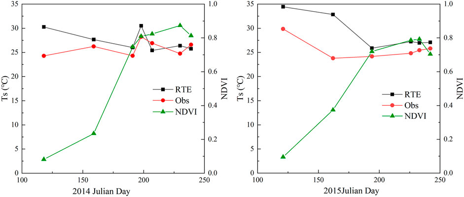
FIGURE 3. Surface temperature (Ts °C) computed from the Radiative Transfer Equation (RTE) method and observed (Obs) from 2015 and 2014. As reference, the normalized difference vegetation index (NDVI) is included from Julian Day 100 to 250.

Correcting RTE with NDVI, the expression is:

$\begin{array}{c}{\text{Ts}}_{RTE-NDVI}={\text{Ts}}_{RTE}-\frac{0.22}{\text{NDVI}}-1.5\end{array}(11)$

where NDVI is Normalized Difference Vegetation Index; ${\text{Ts}}_{RTE-NDVI}$ is the surface temperature calculated using the Radiation Transfer Equation corrected by NDVI (°C); ${\text{ Ts}}_{RTE}$ is the surface temperature calculated using the original Radiation Transfer Equation (°C).

The 31 measured data from 2014 to 2017 were used as the target to revise the RTE (Figure 4A), and the 2018 data were used as verification (Figure 4B). After correction using NDVI of 2014–2017, compared with the verified data, the accuracy of the model is R² = 0.83, RMSE = 2.09°C. And after the verification of the data in 2018, it is confirmed that Eq. 11 has improved the accuracy of RTE (before: R² = 0.63, RMSE = 4.80°C; After: R² = 0.76, RMSE = 2.41°C). The fitting line is close to 1:1, indicating that the estimation accuracy of the Ts is significantly improved.

FIGURE 4

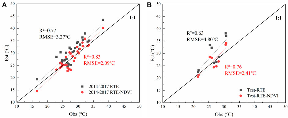
FIGURE 4. Comparison between observed (Obs) and estimated (Est) surface temperature for 2014-2017 (A), 2018 (B). RTE and NDVI-RTE corresponds to the estimated values from the original equation and RTE equation adjusted using the normalized difference vegetation index (NDVI), respectively. Also, coefficients of determination (R2) and root mean square error (RMSE °C) are indicated in the figure.

Variable Importance and Selection

Seven variables were tested for multicollinearity, and there was no variable with VIF greater than 10, indicating that the regression model can be established. As shown in Figure 5, RSS monotonically decreases with the increase of the number of independent variables, which cannot be directly judged. Adjusted R² and Cp values tended to be the largest when the number of variables was 6 and 7. The adjusted R² for Ta models ranged from 0.87 to 0.95, which eventually fixed at 0.95. Further addition of the independent variable did not improve the adjusted R², indicating that 6 independent variables were considered optimal. The change of BIC with the number of variables also proves that the model with six variables has the highest accuracy.

FIGURE 5

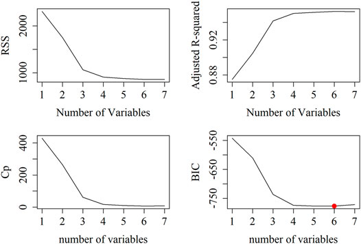
FIGURE 5. Effect of number of variables in the air temperature model on Residual Sum of Squares (RSS), adjusted coefficients of determination (adjusted R²), Mallows’s Cp (Cp) value, and Bayesian Information Criterion (BIC).

The statistical analysis indicated that Ts, Albedo, NDVI, DEM, x7, and x8 were significant independent variables for estimating Ta. As shown in Figure 6, R² was increased with the increase of the independent variables, so optimal combination of independent variables was not proposed in this study. However, in the absence of the wind speed, the adjusted R² reached a maximum while Cp and BIC arrived at a minimum, indicating that wind speed does not improve the accuracy of the Ta model. Except that the wind speed does not affect the model construction, the addition of other variables can improve the fitting accuracy of the model. The date of Ta estimation is almost always sunny when the average wind speed is slightly different in space. Therefore, there is no significant correlation between wind speed and Ta variation. Moreover, the average wind speed data is interpolated from the data obtained from meteorological stations, which may be inaccurate at the regional scale. To sum up, it is sufficient to use remote sensing data, elevation, and Julian days as the independent variables for the model.

FIGURE 6

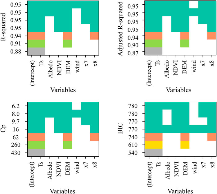
FIGURE 6. Combination of different variables when the value of coefficients of determination (R²), adjusted coefficients of determination (adjusted R²), Mallows's Cp (Cp) value, and Bayesian Information Criterion (BIC) value were stabilized. The variables included surface temperature (Ts), normalized vegetation index (NDVI), surface albedo (Albedo), elevation (DEM), wind speed (wind), $x7={(J-200)}^2$ and $x8=x7\times Ts$. The highest color in the figure indicates that the statistical indicators are gradually stable, and the variable combination is optimal.

After determining the independent variables, the formula of the constructed multiple linear regression equation is as follows:

$\begin{array}{c}Ta=b_0+b_{1}Ts+b_2\alpha +b_{3}NDVI+b_{4}H+b_{5}x7+b_{6}x8\end{array}(12)$

where Ta is the near-surface air temperature; Ts is the surface temperature; a is the surface albedo; NDVI is Normalized Difference Vegetation Index; H is the altitude; $x7={(J-200)}^2; x8 = x7\times Ts$; J is Julian Day (the number of the day of the year); b_0∼b₆ are undetermined coefficients.

The random forest algorithm cannot provide an estimation form similar to MLR because it cannot be parameterized. Two parameters are critical to the operation of the random forest model: the number of trees to grow (ntree) and the number of variables to be used at each node (mtry). These two parameters are selected based on the percentage of model interpretation and mean of squared residuals. The mtry value was tested from 1 to 8, and the ntree value was tested using the following 6 values: 100, 300, 500, 1,000, 1,500, and 2,000.

Figure 7 shows the changes in Mean of squared residuals and Percent variance explained after running a random forest with different ntree and mtry values. The highest Percent variance explained and the lowest Mean of squared residuals were obtained when mtry = 3 and ntree = 1,500 or 2,000. Since the higher the value of ntree, the more cost and time for calculation, so the value of ntree is set to 1,500, and the value of mtry is set to 3 to run the random forest model.

FIGURE 7

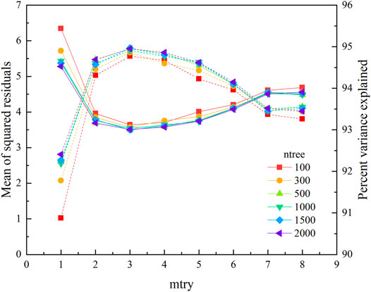
FIGURE 7. Mean of squared residuals and variation in percentage variance explained by the random forest model with different number of trees to grow (ntree) and number of variables to be used at each node (mtry). Dotted lines represent percentage variance explained; solid lines represent Mean of squared residuals.

The amount of Ta-related data from 2014 to 2019 is 397. Randomly select 70% of the total amount as the training set to determine the variables and parameters, and the remaining data as the testing set. Figure 8 is a scatter plot of the simulated and observed values of the two models constructed from the training set data. The R² and RMSE of the MLR model were 0.953 and 1.74°C, respectively. Most of the points of the RF are concentrated and close to the 1:1 line. The comparison between the results of the RF model and the MLR model shows that the random forest has higher estimation accuracy.

FIGURE 8

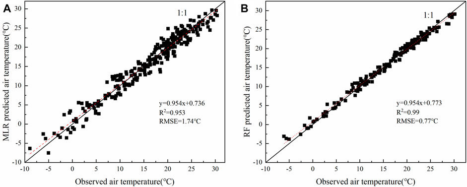
FIGURE 8. Scatter plot between predicted and in-situ near-surface air temperatures (Ta °C) based on multiple linear regression (MLR) model (Figure 8A) and random forest (RF) algorithm (Figure 8b). The surface temperature (Ts °C) in the models is calculated by radiation transfer equation (RTE). Coefficients of determination (R²) and root mean square error (RMSE °C) were used to evaluate the accuracy of Ta estimation from the training set.

Model Validation

To understand the universality of the built model, the MLR model was verified using the 2018–2019 dataset; the RF algorithm was verified using the reserved test dataset. At the same time, it is explored whether the improvement of the estimation accuracy of Ts will affect the estimation accuracy of Ta.

The prediction result of Ta estimated through the validation data set (Figure 9) cannot reach the accuracy of the initial training set. When Ta is estimated from the validation data set of the RF, the prediction could not achieve the accuracy of the initial training set, respectively. When using NDVI to correct RTE, the R² and RMSE of the RF model was 0.943 and 2.12°C, respectively, indicating that the estimation accuracy of using RTE-NDVI is reduced. In contrast, the simulation results of MLR on Ta are relatively stable. The two calculation methods of Ts have little effect on MLR. Therefore, the accuracy of Ts inversion will not affect the accuracy of the two methods for estimating Ta. The estimation results of all models show good performance, and the fitting line is close to 1:1.

FIGURE 9

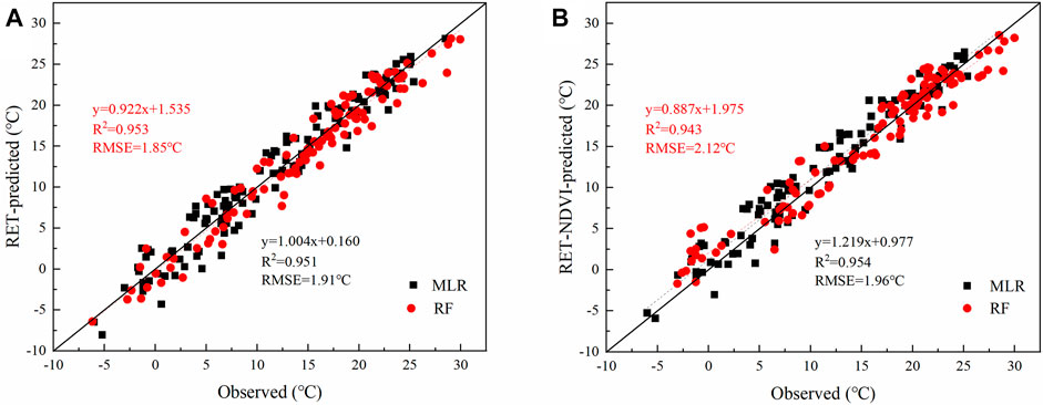
FIGURE 9. The Ts involved in the Ta estimation were calculated through the radiation transfer equation (RTE, (A)) and the NDVI correction (NDVI-RTE, (B)). The coefficient of determination (R²) and root mean square error (RMSE °C) were used to evaluate the accuracy of estimation Ta on the validation set for the two models and the two Ts data.

Spatial and Temporal Performance

Through the analysis of the average daily Ta and error estimated by MLR for 2018–2019, it was found that the temperature and error on the time scale have spatial variability. As shown in Figure 10, Ta had a clear trend with Julian day and season, and the estimation accuracy had an apparent seasonal trend. Sometimes, the meteorological station is covered by clouds and cannot participate in the calculation or verification, especially at the high-altitude Wushaoling station. The amount of remote sensing image data in winter is insufficient. Although the error is small, it cannot be fully verified. There was not much difference in the accuracy between spring and summer. The RMSE values in spring and summer were both 1.66°C, which had no difference in the estimation accuracy. With the increase of temperature, the error value was relatively stable and had no apparent change trend. In autumn, the RMSE was 2.35°C. At this time, the study area is in the rainy season, and the estimate of Ta will be affected by the increase in rainfall.

FIGURE 10

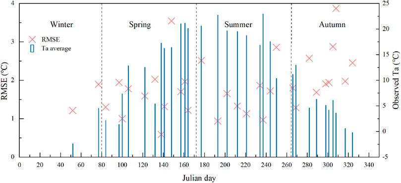
FIGURE 10. Relations between the temporal distribution of observed near-surface air temperature (Ta °C) and model performance, using root mean square error (RMSE °C) to represent the accuracy in the estimation of air temperature (Ta).

In 2018 and 2019, the MEF value of each station was between 0.84 and 0.97, and the overall MEF was 0.946, indicating that MLR has good performance. Analyze the error distribution of Ta estimated by the MLR model at each site. Figure 9 shows that Ta is more accurate at locations far from the mountainous area.

The MEF of the Minqin station for 2 years was close to 1, and the degree of the fitting was relatively high. The MLR model behaved differently in different altitude ranges. As the altitude increases, the performance of the MLR model gradually weakens, which may be caused by the complexity of the terrain. The RMSE has the maximum value at the highest altitude site (Wu Shaolin) (Figures 11C,D). The average RMSE of Minqin and Jintai Station are below 1.5°C. The accuracy of these two stations is better than that of other stations, possibly because the terrain and environmental conditions of the stations are not complicated. The locations of these two stations are far away from the Qilian Mountains, which are as high as 5,000 m above sea level. The estimation model had the highest relevance and accuracy at the Minqin station, which is located on the north side of the basin, and the surrounding terrain is flat and less affected by high mountains. Although Jintai Station is close to the east of Qilian Mountain, which is far from the mountain range, the estimation accuracy of Ta is also very high.

FIGURE 11

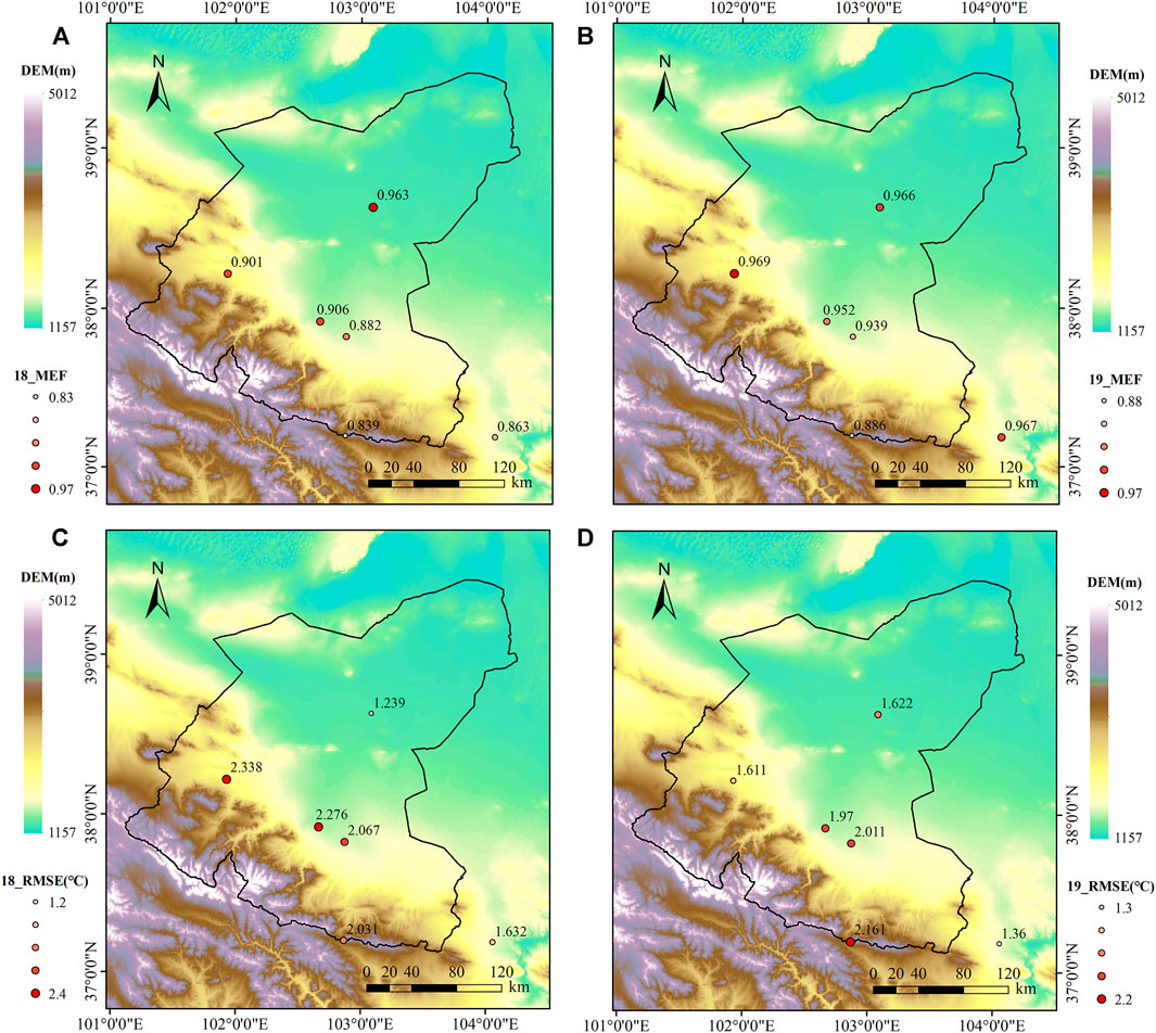
FIGURE 11. Spatial distribution of the optimal models, model efficiency (MEF): (A) 2018, (B) 2019, root mean square error (RMSE °C): (C) 2018, (D) 2019 for all the meteorological stations.

Because the data of the two adjacent columns of the Landsat satellite are of different periods, remote sensing images of the entire study area cannot be obtained on the same day, so the basin can only be divided into two parts for comparison. Chosen four images with fewer clouds, then calculated the difference between the spatial interpolation result and the MLR model estimate. Inverse Distance Weighted (IDW) assumes that the influence of variables on the surrounding area decreases as the distance to the sample location increases, which was used to interpolate Ta data from the meteorological station. The error of Ta distribution obtained by IDW in the area is related to the underlying surface. Using meteorological and remote sensing data from July 31, August 22, 2018, May 21, May 28, 2019, Ta spatial interpolation and estimation maps were obtained and compared.

It iswidely believed that Ta is related to altitude. Temperature decreased with the increase of altitude in most cases. In high altitude areas, where no meteorological station provides temperature data, the Ta of the regions was determined by data from nearby stations. Therefore, Ta in high altitude areas was often overestimated by interpolation (the red area below Figures 12A,C). Simultaneously, there are also large desert areas in the study area (the blue area in Figure 12). Since the temperature in the desert during the day will be much higher than in other zones, the interpolation method can underestimate the temperature by up to 15°C. The Ta of farmland is overestimated during spatial interpolation (the part of the red area above d in Figure 12B), which is also related to the location of meteorological stations. Most of the station is established in cities or border areas. The vegetation coverage of farmland is very high during the growth period of crops, which will affect its Ta. Therefore, when using interpolation methods such as IDW, more meteorological stations are needed to ensure the accuracy of the interpolation results, and at the same time, should pay attention to the unreliability of interpolation methods in mountains or deserts.

FIGURE 12

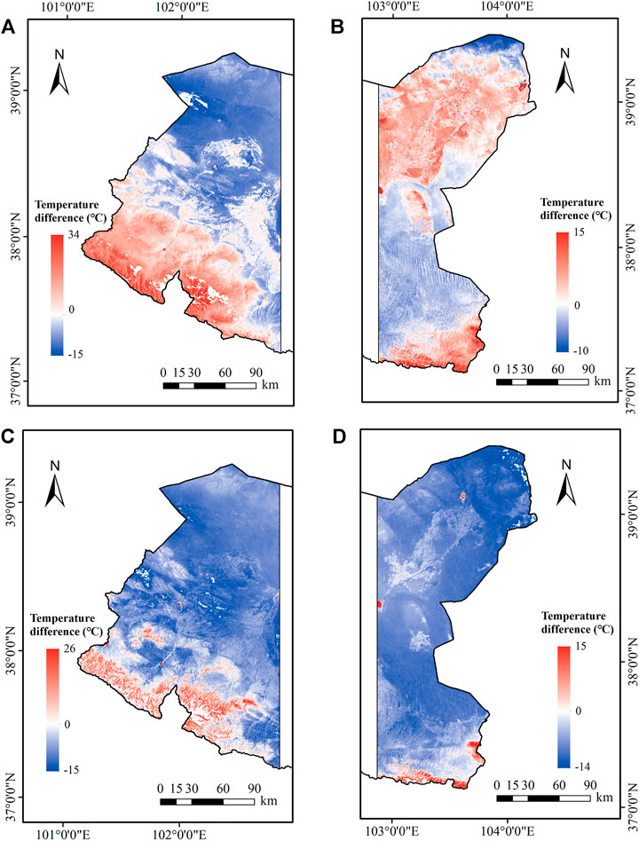
FIGURE 12. Difference between interpolation method and multiple linear regression model estimation result (A-D): (July 31 and August 22, 2018, and May 21 and May 28, 2019).

Discussion

Model Selection

In areas with vegetation cover, the temperature value retrieved from remote sensing data is often a mixed value of Ts and canopy temperature (Tc). The accurate estimation of Ts still needs to be analyzed according to the vegetation situation and terrain (Zhang and Li, 2018). Comparing the Ts calculated by RTE with the measured values, it was found that RTE overestimated the Ts, especially when the vegetation coverage was low, consistent with the conclusions published by USGS in 2015 (Barsi et al., 2014; Xu and Huang, 2016). However, due to the characteristics of fewer parameters and suitable for any thermal infrared band, the improved accuracy can also be widely used. Ts is considered to be the most important independent variable the many estimated Ta models (Park, 2011; Zhang et al., 2016; Song and Wu, 2018). In this study, the RMSE of Ts directly calculated by RTE is 3–5°C, and it is 2–3°C after correction. The correction equation is proposed based on the local estimation results, and its universality still needs to be verified. The error is related to the surface emissivity or atmospheric profile parameters (Li et al., 2013; Sekertekin and Bonafoni, 2020).

The variables of this study to be selected are closely related to Ta in many studies (Cristóbal et al., 2008; Gholamnia et al., 2017; Shen et al., 2020). Although the correlation between time parameters and Ta was not strong, the adjusted x7 had a significant influence on model accuracy indicating that the adjustment using the Julian Day was useful. Studies have suggested that wind speed is significant, especially when using energy balance methods, which require wind speed to calculate aerodynamic resistance (Hou et al., 2013; Zhang et al., 2015). Through indicators comparison, it is found that when using a statistical method to build the model, the average wind speed is not helpful to improve Ta estimation accuracy (Stisen et al., 2007).

The selected variables participate in MLR and RF to estimate Ta, using the available satellite dataset. The RMSE of the two methods were both lower than 2.0°C, which indicated that they were both suitable for northwest China. Previously, Ho et al. (2014) Using the RF algorithm to estimate the maximum Ta in Vancouver, Canada, and the RMSE was 2.3°C. The optimal MLR model established by Yang et al. (2017) estimates the average Ta and the RMSE is 3.6°C. Therefore, the methods of estimating Ta in this study had relatively high accuracy. However, due to the 16-days revisit cycle of the Landsat satellite and the low temporal resolution of the images, there are limitations in monitoring daily Ta (Yoo et al., 2018).

When performing regression, the random forest cannot make predictions that exceed the range of the training dataset, which may lead to overfitting when modeling some data with specific noise. For many statistical modelers, the random forest is like a black box (Zheng et al., 2019), almost unable to control the internal operation of the model, can only try between different parameters and random allocation. The simulation results of the random forest algorithm for the existing data are very good, but when it is used in the prediction and estimation, its accuracy may drop suddenly. It is difficult to improve it because it cannot control the internal operation of the model. For this study, multiple linear regression is still recommended. The simulation accuracy of the MLR model is similar to that of validation, which is conducive to the evaluation of subsequent prediction results. From the comparison results of the models, the MLR and RF models that without improving the accuracy of Ts performed better, and the actual operation was simpler. The reason for this phenomenon may be that the NDVI involved in the Ts correction is also one of the independent variables of the Ta estimation model, which makes the internal adjustment of the model during operation can ignore the errors of Ts.

Spatial and Temporal Uncertainties of Model

The seasonal variation of the average temperature and the distribution of the station will affect the estimation accuracy of Ta (Holden et al., 2011; Chen et al., 2015). From the time point of view, the RMSE in autumn reaches 2.24°C, which is 0.57°C higher than that in spring and summer. This is consistent with the results of Golkar et al. (2018), which believe that the estimation of Ta in spring and summer has higher accuracy, while there are more uncertainties in autumn. Therefore, the estimation model of daily average temperature is more suitable for spring and summer days. Yang et al. (2017) integrated various statistical indicators and believed that each model performed better in spring, and the estimation accuracy decreased due to the influence of rainfall and cloudy weather. The study area is located in the inland of Northwest China, and rainfall is mainly concentrated in autumn. Benali et al. (2012) believe that the cloud cover of remote sensing images is inversely proportional to the model performance, and higher cloud cover harms model performance. That is, because cloud cover could reduce the accuracy of the Ts, which affects the accuracy of estimated values of daily average temperature. Therefore, the model can be optimized to the season or month scale, and the process of climate and environmental impacts can be added to adapt to the impact of climate change and cloud cover.

The spatial distribution map of RMSE shows that the model in mountainous and plateau areas generally performs worse than in plain areas. This conclusion is consistent with the research results of Yang et al. (2017). Due to the influence of terrain differences, mountainous terrain has a broader spatial variation range than flat terrain, so mountain temperature changes are more complicated. On relatively flat terrain and vegetation, horizontal uniformity leads to stable atmospheric conditions (Blandford et al., 2008; Lin et al., 2016). Ta raster data is usually limited by site coverage, especially in mountainous areas where the density and elevation distribution of meteorological observations vary greatly (Holden et al., 2011). Shen et al. (2020) believe that in the case of large-scale use of MLR and RF, the accuracy of the estimation results is poor due to the scarcity of sites in Northwest China that can participate in model training. When MLR is estimated in the Shiyang River Basin, the MEF of the highest altitude station (3000 m) is higher than 0.83, and the RMSE = 2.10°C, the model also performs well.

The method proposed by the research can obtain high-precision Ta estimation results when using the Landsat 8 data set, and improve the spatial resolution. However, the actual situation of only six meteorological stations limits the accuracy of Ta inversion in this area. We hope that more reliable verification data can be obtained in future studies.

Conclusion

The purpose of this study is to estimate Ts and Ta in the Shiyang River Basin. Perform parameter inversion based on Landsat8 images, use RTE to calculate and correct Ts. Using Ts, NDVI, elevation, and other parameters as variables to construct MLR and RF models for estimating Ta. The results show that: For MLR and RF, after calibrating Ts and participating in the estimation of Ta, both methods have accurate estimation results; The accuracy of RF training results is better than MLR, but the test set results of the two models are not significantly different; Although the topography of the study area is complex and the land cover conditions are different, the MLR model applies to the study area. In addition, compared with the MLR model, the comparison found that the interpolation method will underestimate the temperature in areas with low vegetation coverage like deserts, while the opposite is in the mountains and farmland areas.

This study can be used to accurately understand the distribution characteristics and changing trends of Ts and Ta in the study area. Further research can optimize the model in time to a month to adapt the climate change; make up the deficiency of Landsat8 and MODIS data by fusing remote sensing data, then obtaining Ta data with high temporal and spatial resolution.

Data Availability Statement

The raw data supporting the conclusion of this article will be made available by the authors, without undue reservation.

Author Contributions

YL and SW conceived the idea. YL wrote the manuscript, SO, FT, and SW revised and improved the paper. The validation data of the model is provided by SL. All authors reviewed the manuscript.

Funding

This study was supported by the International and regional cooperation and exchange projects of the National Natural Science Foundation of China (51961125205), and the Chilean government through National Agency for Research and Development (ANID)/PCI (NSFC190013).

Conflict of Interest

The authors declare that the research was conducted in the absence of any commercial or financial relationships that could be construed as a potential conflict of interest.

Publisher’s Note

All claims expressed in this article are solely those of the authors and do not necessarily represent those of their affiliated organizations, or those of the publisher, the editors and the reviewers. Any product that may be evaluated in this article, or claim that may be made by its manufacturer, is not guaranteed or endorsed by the publisher.

Acknowledgments

The authors would like to thank the NASA team for making the remote sensing data freely available, the GEE platform for processing remote sensing data, and the National Meteorological Information Center of China Meteorological Administration for archiving the observed climate data (http://data.cma.cn).

References

Agha, S. R., and Alnahhal, M. J. (2012). Neural Network and Multiple Linear Regression to Predict School Children Dimensions for Ergonomic School Furniture Design. Appl. Ergon. 43, 979–984. doi:10.1016/j.apergo.2012.01.007

PubMed Abstract | CrossRef Full Text | Google Scholar

Akan, R., Keskin, S. N., and Uzundurukan, S. (2015). Multiple Regression Model for the Prediction of Unconfined Compressive Strength of Jet Grout Columns. Proced. Earth Planet. Sci. 15, 299–303. doi:10.1016/j.proeps.2015.08.072

CrossRef Full Text | Google Scholar

Alkama, R., and Cescatti, A. (2016). Biophysical Climate Impacts of Recent Changes in Global forest Cover. Science 351, 600–604. doi:10.1126/science.aac8083

PubMed Abstract | CrossRef Full Text | Google Scholar

Anderson, M., Norman, J., Kustas, W., Houborg, R., Starks, P., and Agam, N. (2008). A thermal-based Remote Sensing Technique for Routine Mapping of Land-Surface Carbon, Water and Energy Fluxes from Field to Regional Scales. Remote Sensing Environ. 112, 4227–4241. doi:10.1016/j.rse.2008.07.009

CrossRef Full Text | Google Scholar

Bai, Y., Wu, L., Qin, K., Zhang, Y., Shen, Y., and Zhou, Y. (2016). A Geographically and Temporally Weighted Regression Model for Ground-Level PM2.5 Estimation from Satellite-Derived 500 M Resolution AOD. Remote Sensing 8, 262. doi:10.3390/rs8030262

CrossRef Full Text | Google Scholar

Barsi, J., Schott, J., Hook, S., Raqueno, N., Markham, B., and Radocinski, R. (2014). Landsat-8 thermal Infrared Sensor (TIRS) Vicarious Radiometric Calibration. Remote Sensing 6, 11607–11626. doi:10.3390/rs61111607

CrossRef Full Text | Google Scholar

Bathiany, S., Dakos, V., Scheffer, M., and Lenton, T. M. (2018). Climate Models Predict Increasing Temperature Variability in Poor Countries. Sci. Adv. 4, 1–11. doi:10.1126/sciadv.aar5809

CrossRef Full Text | Google Scholar

Becker, W. R., Ló, T. B., Johann, J. A., and Mercante, E. (2021). Statistical Features for Land Use and Land Cover Classification in Google Earth Engine. Remote Sensing Appl. Soc. Environ. 21, 100459. doi:10.1016/j.rsase.2020.100459

CrossRef Full Text | Google Scholar

Benali, A., Carvalho, A. C., Nunes, J. P., Carvalhais, N., and Santos, A. (2012). Estimating Air Surface Temperature in Portugal Using MODIS LST Data. Remote Sensing Environ. 124, 108–121. doi:10.1016/j.rse.2012.04.024

CrossRef Full Text | Google Scholar

Blandford, T. R., Humes, K. S., Harshburger, B. J., Moore, B. C., Walden, V. P., and Ye, H. (2008). Seasonal and Synoptic Variations in Near-Surface Air Temperature Lapse Rates in a Mountainous basin. J. Appl. Meteorol. Climatol. 47, 249–261. doi:10.1175/2007JAMC1565.1

CrossRef Full Text | Google Scholar

Breiman, L. (2001). Random Forests. Mach. Learn. 45, 5–32. doi:10.1023/A:1010933404324

CrossRef Full Text | Google Scholar

Chen, F., Liu, Y., Liu, Q., and Qin, F. (2015). A Statistical Method Based on Remote Sensing for the Estimation of Air Temperature in China. Int. J. Climatol 35, 2131–2143. doi:10.1002/joc.4113

CrossRef Full Text | Google Scholar

Cresswell, M. P., Morse, A. P., Thomson, M. C., and Connor, S. J. (1999). Estimating Surface Air Temperatures, from Meteosat Land Surface Temperatures, Using an Empirical Solar Zenith Angle Model. Int. J. Remote Sensing 20, 1125–1132. doi:10.1080/014311699212885

CrossRef Full Text | Google Scholar

Cristóbal, J., Ninyerola, M., and Pons, X. (2008). Modeling Air Temperature through a Combination of Remote Sensing and GIS Data. J. Geophys. Res. 113, 1–13. doi:10.1029/2007JD009318

CrossRef Full Text | Google Scholar

Czajkowski, K. P., Mulhern, T., Goward, S. N., Cihlar, J., Dubayah, R. O., and Prince, S. D. (1997). Biospheric Environmental Monitoring at BOREAS with AVHRR Observations. J. Geophys. Res. 102, 29651–29662. doi:10.1029/97jd01327

CrossRef Full Text | Google Scholar

Emamifar, S., Rahimikhoob, A., and Noroozi, A. A. (2013). Daily Mean Air Temperature Estimation from MODIS Land Surface Temperature Products Based on M5 Model Tree. Int. J. Climatol. 33, 3174–3181. doi:10.1002/joc.3655

CrossRef Full Text | Google Scholar

Farr, T. G., Rosen, P. A., Caro, E., Crippen, R., Duren, R., Hensley, S., et al. (2007). The Shuttle Radar Topography Mission. Rev. Geophys. 45, RG2004. doi:10.1029/2005RG000183

CrossRef Full Text | Google Scholar

Folland, C. K., Boucher, O., Colman, A., and Parker, D. E. (2018). Causes of Irregularities in Trends of Global Mean Surface Temperature since the Late 19th century. Sci. Adv. 4. doi:10.1126/sciadv.aao5297

PubMed Abstract | CrossRef Full Text | Google Scholar

Genuer, R., Poggi, J.-M., Tuleau-Malot, C., and Villa-Vialaneix, N. (2017). Random Forests for Big Data. Big Data Res. 9, 28–46. doi:10.1016/j.bdr.2017.07.003

CrossRef Full Text | Google Scholar

Gholamnia, M., Darvishi Boloorani, A., Hamzeh, S., Kiavarz, M., and Kiavarz, M. (2017). Diurnal Air Temperature Modeling Based on the Land Surface Temperature. Remote Sensing 9, 915. doi:10.3390/rs9090915

CrossRef Full Text | Google Scholar

Giacomino, A., Abollino, O., Malandrino, M., and Mentasti, E. (2011). The Role of Chemometrics in Single and Sequential Extraction Assays: A Review. Part II. Cluster Analysis, Multiple Linear Regression, Mixture Resolution, Experimental Design and Other Techniques. Analytica Chim. Acta 688, 122–139. doi:10.1016/j.aca.2010.12.028

PubMed Abstract | CrossRef Full Text | Google Scholar

Golkar, F., Sabziparvar, A. A., Khanbilvardi, R., Nazemosadat, M. J., Zand- Parsa, S., and Rezaei, Y. (2018). Estimation of Instantaneous Air Temperature Using Remote Sensing Data. Int. J. Remote Sensing 39, 258–275. doi:10.1080/01431161.2017.1382743

CrossRef Full Text | Google Scholar

Goward, S. N., Waring, R. H., Dye, D. G., and Yang, J. (1994). Ecological Remote Sensing at OTTER: Satellite Macroscale Observations. Ecol. Appl. 4, 322–343. doi:10.2307/1941937

CrossRef Full Text | Google Scholar

Hachem, S., Duguay, C. R., and Allard, M. (2012). Comparison of MODIS-Derived Land Surface Temperatures with Ground Surface and Air Temperature Measurements in Continuous Permafrost Terrain. The Cryosphere 6, 51–69. doi:10.5194/tc-6-51-2012

CrossRef Full Text | Google Scholar

Ho, H. C., Knudby, A., Sirovyak, P., Xu, Y., Hodul, M., and Henderson, S. B. (2014). Mapping Maximum Urban Air Temperature on Hot Summer Days. Remote Sensing Environ. 154, 38–45. doi:10.1016/j.rse.2014.08.012

CrossRef Full Text | Google Scholar

Holden, Z. A., Abatzoglou, J. T., Luce, C. H., and Baggett, L. S. (2011). Empirical Downscaling of Daily Minimum Air Temperature at Very fine Resolutions in Complex Terrain. Agric. For. Meteorology 151, 1066–1073. doi:10.1016/j.agrformet.2011.03.011

CrossRef Full Text | Google Scholar

Hou, P., Chen, Y., Qiao, W., Cao, G., Jiang, W., and Li, J. (2013). Near-surface Air Temperature Retrieval from Satellite Images and Influence by Wetlands in Urban Region. Theor. Appl. Climatol. 111, 109–118. doi:10.1007/s00704-012-0629-7

CrossRef Full Text | Google Scholar

Isaya Ndossi, M., and Avdan, U. (2016). Application of Open Source Coding Technologies in the Production of Land Surface Temperature (LST) Maps from Landsat: A PyQGIS Plugin. Remote Sensing 8, 413. doi:10.3390/rs8050413

CrossRef Full Text | Google Scholar

James, G., Witten, D., Hastie, T., and Tibshirani, R. (2013). An Introduction to Statistical Learning: With Applications in R. 1st ed. New YorkNew York: Springer.

Google Scholar

Jang, J.-D., Viau, A. A., and Anctil, F. (2004). Neural Network Estimation of Air Temperatures from AVHRR Data. Int. J. Remote Sensing 25, 4541–4554. doi:10.1080/01431160310001657533

CrossRef Full Text | Google Scholar

Janssen, P. H. M., and Heuberger, P. S. C. (1995). Calibration of Process-Oriented Models. Ecol. Model. 83, 55–66. doi:10.1016/0304-3800(95)00084-9

CrossRef Full Text | Google Scholar

Jimenez-Munoz, J. C., Cristobal, J., Sobrino, J. A., Soria, G., Ninyerola, M., Pons, X., et al. (2009). Revision of the Single-Channel Algorithm for Land Surface Temperature Retrieval from Landsat thermal-infrared Data. IEEE Trans. Geosci. Remote Sensing 47, 339–349. doi:10.1109/TGRS.2008.2007125

CrossRef Full Text | Google Scholar

Ke, Y., Im, J., Park, S., and Gong, H. (2016). Downscaling of MODIS One Kilometer Evapotranspiration Using Landsat-8 Data and Machine Learning Approaches. Remote Sensing 8, 215–226. doi:10.3390/rs8030215

CrossRef Full Text | Google Scholar

Krüger, E., and Emmanuel, R. (2013). Accounting for Atmospheric Stability Conditions in Urban Heat Island Studies: The Case of Glasgow, UK. Landscape Urban Plann. 117, 112–121. doi:10.1016/j.landurbplan.2013.04.019

CrossRef Full Text | Google Scholar

Li, L., and Zha, Y. (2018). Mapping Relative Humidity, Average and Extreme Temperature in Hot Summer over China. Sci. Total Environ. 615, 875–881. doi:10.1016/j.scitotenv.2017.10.022

PubMed Abstract | CrossRef Full Text | Google Scholar

Li, S., Quackenbush, L. J., and Im, J. (2019). Airborne Lidar Sampling Strategies to Enhance forest Aboveground Biomass Estimation from Landsat Imagery. Remote Sensing 11, 1906. doi:10.3390/rs11161906

CrossRef Full Text | Google Scholar

Li, X., Zhou, Y., Asrar, G. R., and Zhu, Z. (2018). Developing a 1 Km Resolution Daily Air Temperature Dataset for Urban and Surrounding Areas in the Conterminous United States. Remote Sensing Environ. 215, 74–84. doi:10.1016/j.rse.2018.05.034

CrossRef Full Text | Google Scholar

Li, Z.-L., Tang, B.-H., Wu, H., Ren, H., Yan, G., Wan, Z., et al. (2013). Satellite-derived Land Surface Temperature: Current Status and Perspectives. Remote Sensing Environ. 131, 14–37. doi:10.1016/j.rse.2012.12.008

CrossRef Full Text | Google Scholar

Liang, S., Shuey, C. J., Russ, A. L., Fang, H., Chen, M., Walthall, C. L., et al. (2003). Narrowband to Broadband Conversions of Land Surface Albedo: II. Validation. Remote Sensing Environ. 84, 25–41. doi:10.1016/S0034-4257(02)00068-8

CrossRef Full Text | Google Scholar

Liaw, A., and Wiener, M. (2015). randomForest: Breiman and Cutler’s Random Forests for Classification and Regression.

Google Scholar

Lin, X., Zhang, W., Huang, Y., Sun, W., Han, P., Yu, L., et al. (2016). Empirical Estimation of Near-Surface Air Temperature in China from MODIS LST Data by Considering Physiographic Features. Remote Sensing 8, 629. doi:10.3390/rs8080629

CrossRef Full Text | Google Scholar

Ma, S., and Pu, Z. (2020). Research on Surface Temperature Inversion Algorithm Based on Landsat8 Data in Urumqi City. Comput. Digit. Eng. 10, 2316–2320. doi:10.3969/j.issn.1672-9722.2020.10.003

CrossRef Full Text | Google Scholar

Meyer, H., Katurji, M., Appelhans, T., Müller, M., Nauss, T., Roudier, P., et al. (2016). Mapping Daily Air Temperature for Antarctica Based on MODIS LST. Remote Sensing 8, 732. doi:10.3390/rs8090732

CrossRef Full Text | Google Scholar

Moser, G., De Martino, M., and Serpico, S. B. (2015). Estimation of Air Surface Temperature from Remote Sensing Images and Pixelwise Modeling of the Estimation Uncertainty through Support Vector Machines. IEEE J. Sel. Top. Appl. Earth Observations Remote Sensing 8, 332–349. doi:10.1109/JSTARS.2014.2361862

CrossRef Full Text | Google Scholar

Mostovoy, G. V., King, R. L., Reddy, K. R., Kakani, V. G., and Filippova, M. G. (2006). Statistical Estimation of Daily Maximum and Minimum Air Temperatures from MODIS LST Data over the State of Mississippi. GIScience & Remote Sensing 43, 78–110. doi:10.2747/1548-1603.43.1.78

CrossRef Full Text | Google Scholar

Nash, J. E., and Sutcliffe, J. V. (1970). River Flow Forecasting through Conceptual Models Part III - the Ray Catchment at Grendon Underwood. J. Hydrol. 11, 109–128. doi:10.1016/0022-1694(70)90098-3

CrossRef Full Text | Google Scholar

Nemani, R. R., and Running, S. W. (1989). Estimation of Regional Surface Resistance to Evapotranspiration from NDVI and Thermal-IR AVHRR Data. J. Appl. Meteorol. 28, 276–284. doi:10.1175/1520-0450(1989)028<0276

CrossRef Full Text | Google Scholar

Nieto, H., Sandholt, I., Aguado, I., Chuvieco, E., and Stisen, S. (2011). Air Temperature Estimation with MSG-SEVIRI Data: Calibration and Validation of the TVX Algorithm for the Iberian Peninsula. Remote Sensing Environ. 115, 107–116. doi:10.1016/j.rse.2010.08.010

CrossRef Full Text | Google Scholar

Noi, P., Degener, J., and Kappas, M. (2017). Comparison of Multiple Linear Regression, Cubist Regression, and Random forest Algorithms to Estimate Daily Air Surface Temperature from Dynamic Combinations of MODIS LST Data. Remote Sensing 9, 398. doi:10.3390/rs9050398

CrossRef Full Text | Google Scholar

Orhan, O., Ekercin, S., and Dadaser-Celik, F. (2014). Use of Landsat Land Surface Temperature and Vegetation Indices for Monitoring Drought in the Salt Lake Basin Area, Turkey. Scientific World J. 2014, 1–11. doi:10.1155/2014/142939

PubMed Abstract | CrossRef Full Text | Google Scholar

Orhan, O., and Yakar, M. (2016). Investigating Land Surface Temperature Changes Using Landsat Data in Konya, Turkey. Int. Arch. Photogramm. Remote Sens. Spat. Inf. Sci. XLI-B8, 285–289. doi:10.5194/isprsarchives-XLI-B8-285-2016

CrossRef Full Text | Google Scholar

Park, S., Im, J., Jang, E., and Rhee, J. (2016). Drought Assessment and Monitoring through Blending of Multi-Sensor Indices Using Machine Learning Approaches for Different Climate Regions. Agric. For. Meteorology 216, 157–169. doi:10.1016/j.agrformet.2015.10.011

CrossRef Full Text | Google Scholar

Park, S. (2011). Integration of Satellite-Measured LST Data into Cokriging for Temperature Estimation on Tropical and Temperate Islands. Int. J. Climatol. 31, 1653–1664. doi:10.1002/joc.2185

CrossRef Full Text | Google Scholar

Park, S., Seo, E., Kang, D., Im, J., and Lee, M.-I. (2018). Prediction of Drought on Pentad Scale Using Remote Sensing Data and MJO index through Random forest over East Asia. Remote Sensing 10, 1811–1818. doi:10.3390/rs10111811

CrossRef Full Text | Google Scholar

Prince, S. D., Goetz, S. J., Dubayah, R. O., Czajkowski, K. P., and Thawley, M. (1998). Inference of Surface and Air Temperature, Atmospheric Precipitable Water and Vapor Pressure Deficit Using Advanced Very High-Resolution Radiometer Satellite Observations: Comparison with Field Observations. J. Hydrol. 212-213, 230–249. doi:10.1016/S0022-1694(98)00210-8

CrossRef Full Text | Google Scholar

R Core Development Team (2008). R: A Language and Environment for Statistical Computing.

Google Scholar

Raja Reddy, K., Hodges, H. F., and Mckinion, J. M. (1997). Crop Modeling and Applications: A Cotton Example. Adv. Agron. 59, 225–290. doi:10.1016/S0065-2113(08)60056-5

CrossRef Full Text | Google Scholar

Richardson, H. J., Hill, D. J., Denesiuk, D. R., and Fraser, L. H. (2017). A Comparison of Geographic Datasets and Field Measurements to Model Soil Carbon Using Random Forests and Stepwise Regressions (British Columbia, Canada). GIScience & Remote Sensing 54, 573–591. doi:10.1080/15481603.2017.1302181

CrossRef Full Text | Google Scholar

Riddering, J. P., and Queen, L. P. (2006). Estimating Near-Surface Air Temperature with NOAA AVHRR. Can. J. Remote Sensing 32, 33–43. doi:10.5589/m06-004

CrossRef Full Text | Google Scholar

Ruiz-Álvarez, M., Alonso-Sarria, F., and Gomariz-Castillo, F. (2019). Interpolation of Instantaneous Air Temperature Using Geographical and MODIS Derived Variables with Machine Learning Techniques. Ijgi 8, 382. doi:10.3390/ijgi8090382

CrossRef Full Text | Google Scholar

Sekertekin, A., and Bonafoni, S. (2020). Land Surface Temperature Retrieval from Landsat 5, 7, and 8 over Rural Areas: Assessment of Different Retrieval Algorithms and Emissivity Models and Toolbox Implementation. Remote Sensing 12, 294. doi:10.3390/rs12020294

CrossRef Full Text | Google Scholar

Shamir, E., and Georgakakos, K. P. (2014). MODIS Land Surface Temperature as an index of Surface Air Temperature for Operational Snowpack Estimation. Remote Sensing Environ. 152, 83–98. doi:10.1016/j.rse.2014.06.001

CrossRef Full Text | Google Scholar

Shen, H., Jiang, Y., Li, T., Cheng, Q., Zeng, C., and Zhang, L. (2020). Deep Learning-Based Air Temperature Mapping by Fusing Remote Sensing, Station, Simulation and Socioeconomic Data. Remote Sensing Environ. 240, 111692. doi:10.1016/j.rse.2020.111692

CrossRef Full Text | Google Scholar

Shabani, A., and Norouzi, M. (2015). Predicting Cation Exchange Capacity by Artificial Neural Network and Multiple Linear Regression Using Terrain and Soil Characteristics. Indian J. Sci. Technol. 8. doi:10.17485/ijst/2015/v8i28/83328

CrossRef Full Text | Google Scholar

Shi, L., Liu, P., Kloog, I., Lee, M., Kosheleva, A., and Schwartz, J. (2016). Estimating Daily Air Temperature across the Southeastern United States Using High-Resolution Satellite Data: A Statistical Modeling Study. Environ. Res. 146, 51–58. doi:10.1016/j.envres.2015.12.006

PubMed Abstract | CrossRef Full Text | Google Scholar

Sobrino, J. A., Jiménez-Muñoz, J. C., and Paolini, L. (2004). Land Surface Temperature Retrieval from LANDSAT TM 5. Remote Sensing Environ. 90, 434–440. doi:10.1016/j.rse.2004.02.003

CrossRef Full Text | Google Scholar

Song, Y., and Wu, C. (2018). Examining Human Heat Stress with Remote Sensing Technology. GIScience & Remote Sensing 55, 19–37. doi:10.1080/15481603.2017.1354804

CrossRef Full Text | Google Scholar

Stisen, S., Sandholt, I., Nørgaard, A., Fensholt, R., and Eklundh, L. (2007). Estimation of Diurnal Air Temperature Using MSG SEVIRI Data in West Africa. Remote Sensing Environ. 110, 262–274. doi:10.1016/j.rse.2007.02.025

CrossRef Full Text | Google Scholar

Vancutsem, C., Ceccato, P., Dinku, T., and Connor, S. J. (2010). Evaluation of MODIS Land Surface Temperature Data to Estimate Air Temperature in Different Ecosystems over Africa. Remote Sensing Environ. 114, 449–465. doi:10.1016/j.rse.2009.10.002

CrossRef Full Text | Google Scholar

Vázquez, D. P., Reyes, F. J. O., and Arboledas, L. A. (1997). A Comparative Study of Algorithms for Estimating Land Surface Temperature from AVHRR Data. Remote Sens. Environ. 62, 215–222. doi:10.1016/S0034-4257(97)00091-6

CrossRef Full Text | Google Scholar

Vogt, J. V., Viau, A. A., and Paquet, F. (1997). Mapping Regional Air Temperature fields Using Satellite-Derived Surface Skin Temperatures. Int. J. Climatol. 17, 1559–1579. doi:10.1002/(sici)1097-0088

CrossRef Full Text | Google Scholar

Wang, M., He, G., Zhang, Z., Wang, G., Zhang, Z., Cao, X., et al. (2017). Comparison of Spatial Interpolation and Regression Analysis Models for an Estimation of Monthly Near Surface Air Temperature in China. Remote Sensing 9, 1278. doi:10.3390/rs9121278

CrossRef Full Text | Google Scholar

Wang, M. M., He, G. J., Zhang, Z. M., Zhang, Z. J., and Liu, X. G. (2018). Estimation of Monthly Near Surface Air Temperature Using Geographically Weighted Regression in China. Int. Arch. Photogramm. Remote Sens. Spat. Inf. Sci. XLII-3, 1747–1750. doi:10.5194/isprs-archives-XLII-3-1747-2018

CrossRef Full Text | Google Scholar

Wang, W., and Lu, Y. (2018). Analysis of the Mean Absolute Error (MAE) and the Root Mean Square Error (RMSE) in Assessing Rounding Model. IOP Conf. Ser. Mater. Sci. Eng. 324, 012049. doi:10.1088/1757-899X/324/1/012049

CrossRef Full Text | Google Scholar

Wang, Y., Zhou, J., Li, M., and Zhang, X. (2016). Validation of Landsat-8 TIRS LAND Surface Temperature Retrieved from Multiple Algorithms in an Extremely Arid Region. Int. Geosci. Remote Sens. Symp., 6934–6937. doi:10.1109/IGARSS.2016.7730809

CrossRef Full Text | Google Scholar

Williams, C. G., and Ojuri, O. O. (2021). Predictive Modelling of Soils' Hydraulic Conductivity Using Artificial Neural Network and Multiple Linear Regression. SN Appl. Sci. 3, 7. doi:10.1007/s42452-020-03974-7

CrossRef Full Text | Google Scholar

Willmott, C., and Matsuura, K. (2005). Advantages of the Mean Absolute Error (MAE) over the Root Mean Square Error (RMSE) in Assessing Average Model Performance. Clim. Res. 30, 79–82. doi:10.3354/cr030079

CrossRef Full Text | Google Scholar

Windahl, E., and Beurs, K. d. (2016). An Intercomparison of Landsat Land Surface Temperature Retrieval Methods under Variable Atmospheric Conditions Using In Situ Skin Temperature. Int. J. Appl. Earth Observation Geoinformation 51, 11–27. doi:10.1016/j.jag.2016.04.003

CrossRef Full Text | Google Scholar

Xu, H. Q., and Huang, S. L. (2016). A Comparative Study on the Calibration Accuracy of Landsat 8 thermal Infrared Sensor Data. Spectrosc. Spectr. Anal., 1941–1948. doi:10.3964/j.issn.1000-0593(2016)06-1941-08

PubMed Abstract | CrossRef Full Text | Google Scholar

Xu, H. Q. (2015). Retrieval of the Reflectance and Land Surface Temperature of the Newly-Launched Landsat 8 Satellite. Chin. J. Geophys. Chin. Ed. 58, 741–747. doi:10.6038/cij20150304

CrossRef Full Text | Google Scholar

Xu, Y., Qin, Z., and Shen, Y. (2012). Study on the Estimation of Near-Surface Air Temperature from MODIS Data by Statistical Methods. Int. J. Remote Sensing 33, 7629–7643. doi:10.1080/01431161.2012.701351

CrossRef Full Text | Google Scholar

Yang, Y., Cai, W., and Yang, J. (2017). Evaluation of MODIS Land Surface Temperature Data to Estimate Near-Surface Air Temperature in Northeast China. Remote Sensing 9, 410–419. doi:10.3390/rs9050410

CrossRef Full Text | Google Scholar

Yoo, C., Im, J., Park, S., and Quackenbush, L. J. (2018). Estimation of Daily Maximum and Minimum Air Temperatures in Urban Landscapes Using MODIS Time Series Satellite Data. ISPRS J. Photogrammetry Remote Sensing 137, 149–162. doi:10.1016/j.isprsjprs.2018.01.018

CrossRef Full Text | Google Scholar

Zakšek, K., and Schroedter-Homscheidt, M. (2009). Parameterization of Air Temperature in High Temporal and Spatial Resolution from a Combination of the SEVIRI and MODIS Instruments. ISPRS J. Photogrammetry Remote Sensing 64, 414–421. doi:10.1016/j.isprsjprs.2009.02.006

CrossRef Full Text | Google Scholar

Zhang, H., Zhang, F., Ye, M., Che, T., and Zhang, G. (2016). Estimating Daily Air Temperatures over the Tibetan Plateau by Dynamically Integrating MODIS LST Data. J. Geophys. Res. Atmos. 121 (11), 11,425–11,441. doi:10.1002/2016JD025154

CrossRef Full Text | Google Scholar

Zhang, R., Rong, Y., Tian, J., Su, H., Li, Z.-L., and Liu, S. (2015). A Remote Sensing Method for Estimating Surface Air Temperature and Surface Vapor Pressure on a Regional Scale. Remote Sensing 7, 6005–6025. doi:10.3390/rs70506005

CrossRef Full Text | Google Scholar

Zhang, X., and Li, P. (2018). A Temperature and Vegetation Adjusted NTL Urban index for Urban Area Mapping and Analysis. ISPRS J. Photogrammetry Remote Sensing 135, 93–111. doi:10.1016/j.isprsjprs.2017.11.016

CrossRef Full Text | Google Scholar

Zheng, L., Jinying, X. U., and Wang, X. (2019). Application of Random Forests Algorithm in Researches on Wetlands. Wetl. Sci. 01, 16–24. doi:10.13248/j.cnki.wetlandsci.2019.01.003

CrossRef Full Text | Google Scholar

Zheng, X., Zhu, J., and Yan, Q. (2013). Monthly Air Temperatures over Northern China Estimated by Integrating MODIS Data with GIS Techniques. J. Appl. Meteorol. Climatol. 52, 1987–2000. doi:10.1175/JAMC-D-12-0264.1

CrossRef Full Text | Google Scholar

Zhu, W., Lű, A., and Jia, S. (2013). Estimation of Daily Maximum and Minimum Air Temperature Using MODIS Land Surface Temperature Products. Remote Sensing Environ. 130, 62–73. doi:10.1016/j.rse.2012.10.034

CrossRef Full Text | Google Scholar