- 1College of Surveying and Geo-Informatics, Tongji University, Shanghai, China
- 2Frontiers Science Center for Intelligent Autonomous Systems, Shanghai, China
- 3School of Geography and Information Engineering, China University of Geosciences (Wuhan), Wuhan, China
- 4National Engineering Research Center of Geographic Information System, China University of Geosciences (Wuhan), Wuhan, China
Sea surface temperature (SST) is an important factor in the global ocean–atmosphere system, being vital in a variety of climate analyses and air–sea interaction research studies. However, estimating daily SST with both high precision and high spatial completeness remains a challenge. This article attempts to solve this problem by merging two complementary daily SST products, that is, the 25 km-resolution Advanced Microwave Scanning Radiometer for EOS (AMSR-E) SST and 4 km-resolution Moderate Resolution Imaging Spectroradiometer (MODIS) SST, using a genetic algorithm–assisted deep neural network model (GA-DNNM). The merged SST with a spatial resolution of 4 km and a temporal resolution of 1 day is achieved. Experiments in the Asia and Indo-Pacific Ocean (AIPO) region in 2005 were conducted to demonstrate the feasibility and advantages of the proposed method. Results showed that the spatial coverages of the original MODIS SST and AMSR-E SST are ranging from 25.0 to 48.1%, and 31.5 to 47.6%, respectively, while the merged SST achieves a spatial coverage ranging from 56.1 to 73.1%, with improvements ranging from 50.2 to 131.7% relative to the original MODIS SST. Comparisons with drifting buoy observations indicate that the merged SST is accurate, with an average bias of 0.006°C and an average RMSE of 0.502°C, in places where the MODIS SST data are missing before being merged in the AIPO area, and with an average bias of −0.082 °C, and an average RMSE of 0.603°C for the merged SST in the whole study area.
Introduction
Sea surface temperature (SST) is an important physical parameter of the oceans, playing a fundamentally important role in the exchange of energy, momentum, and moisture between the oceans and atmosphere (Wentz et al., 2000). The SST’s changes may alter marine ecosystems, affect global climate significantly, influence the development and evolution of tropical storms and hurricanes, and potentially contribute to droughts and floods in some areas (Wentz et al., 2000; USEPA, 2021). SST with high spatiotemporal resolution, spatial coverage, and accuracy is of vital importance to forecasting weather and monitoring climate change (Reynolds & Smith, 1995; Reynolds et al., 2002; Guan & Kawamura, 2004; Guo, 2010; Li et al., 2013; Tang et al., 2015; Zhu et al., 2018; Xiao et al., 2019).
Satellite observations, including infrared (IR) and microwave (MW), are the major sources based on which the global SST products are derived. IR SST is the earliest satellite derived one that emerged in the 1970s (Wentz et al., 2000). The IR SST usually has high spatial resolutions but is vulnerable to cloud contaminations (covering about half of the Earth), fog, and aerosols, leading to sparse spatial coverage and large amounts of missing data (Tang et al., 2015). In contrast, microwaves can penetrate clouds with little attenuation, and thus, MW SST can provide a fairly high spatial coverage of the sea under all weather conditions, except for rain (Wentz et al., 2000). However, MW SST has lower resolution than IR SST. Besides, its accuracy near coastlines is low, and it may not even be retrieved near lands (Li et al., 2013). It can be concluded that both IR SST and MW SST have advantages and disadvantages, which means they can only derive SST under certain circumstances alone. However, they are complementary to each other. Therefore, we can utilize these two types of SST complementarily to obtain SST with desirable qualities based on the idea of synergy (Zhang and Chen, 2016).
There have already been research studies on conflating MW SST and IR SST (Chao et al., 2009; Donlon et al., 2012; Guan & Kawamura, 2004; Guo, 2010; Li et al., 2013; Tang et al., 2015; Wang & Xie, 2007; Zhu et al., 2018). The mostly used methods are objective analysis (OA), optimum interpolation (OI), data assimilation, and Bayesian methods. OA, based on the Gauss–Markov theorem, was first introduced into oceanographic applications by Bretherton et al. (1976). However, statistical information about the field to be interpolated should be known or the field should be smooth (McIntosh, 1990). The OI method can increase the spatial completeness. However, it smoothens the fine spatial characteristics, which limits applications near the coastal area (Li et al., 2013; Tang et al., 2015). Besides, prior knowledge of the statistics of errors of input data is also required, which however is hard to know (Bretherton et al., 1976; Tang et al., 2015). There are primarily two data assimilation methods applied to merging SSTs, including the VARiational (VAR) approach and Kalman filter (KF). Using the same mathematical principle with OI, the VAR approach has a disadvantage that the variances of the background error and the covariances of the observational error are usually subjectively specified due to the difficulties in ascertaining them (Li et al., 2013; Tang et al., 2015). The KF needs to transform scales before merging, which may introduce extra uncertainties (Zhu et al., 2018). The Bayesian hierarchal model (BHM) and Bayesian maximum entropy (BME) are two typical Bayesian methods for merging multiple SSTs. The BHM-based methods assume that the value of pre-fusion data satisfies a special distribution. They use the prior knowledge as parameters and conclude the posterior average value to be the fused value (Guo, 2010). Therefore, prior knowledge is still a necessity, and bad or insufficient prior knowledge may lead to inaccurate fusion results. BME has been successfully applied to merging IR SST and MW SST of different spatial resolutions to produce high-resolution and high-accuracy SST (Li et al., 2013; Tang et al., 2015). The BME method can resolve the scale transformation problem of KF, but prior knowledge is still needed.
Unlike the previous methods, the deep neural network model represents a nonlinear computational method for learning knowledge from data and predicting complex trends, no matter what distributions the errors are subjected to, or how complex the relationships hidden in the data are (Yue et al., 2017; Zare Abyaneh et al., 2016). It has been successfully applied to numerous areas such as speech recognition (Dahl et al., 2012), human face recognition (Le, 2011), crop yield prediction (Kaul et al., 2005; Panda et al., 2010), crop type classification (Cai et al., 2018), weather forecasting (Valverde Ramírez et al., 2005), environmental monitoring (Li et al., 2017), and image fusion (Wu et al., 2018). However, neural networks tend to get trapped in local extreme values during training. Therefore, some researchers have tried to solve this problem by combing the neural network approach with optimization methods such as genetic algorithms (GA), and have achieved better performance and improved results consequently (Mahmoudabadi et al., 2009; Tahmasebi & Hezarkhani, 2012).
Therefore, considering the complex patterns and uncertainties in the satellite data, the fact that current methods usually require prior knowledge about the error statistics of input data which however is sometimes hard to ascertain, and the advantages of genetic algorithm-assisted deep neural network model (GA-DNNM) in learning patterns of data and dealing with uncertainties, no matter how complex the patterns are and how the data are distributed, we adapt the GA-DNNM to model the relationship between IR SST and MW SST data, and merge these two data to produce high-quality SST products which can further benefit climate analyses and air–sea interaction studies. Therefore, this research aims to 1) develop a GA-DNNM model to capture complex relationships between IR SST and MW SST, and evaluate the accuracy of such relationships over different time frames; 2) exploit the relationships to produce merged SST using IR SST and MW SST; and 3) evaluate the quality of the merged SST with drifting buoy observations (ground truth).
The study area is targeted at the area joined by the Asia and Indo-Pacific Ocean (AIPO) (Chang-Xiang et al., 2010). The major contributions of this article include 1) a novel GA-DNNM method specifically developed and demonstrated to be feasible and accurate for the task of merging IR SST and MW SST, and 2) the merged SST whose spatial resolution is 4 km, temporal resolution is 1 day, and spatial coverage is much improved.
The reminder of the article is structured as follows. In Section 2, the study area and data are introduced. Section 3 describes the method, including data preprocessing, deep neural network model design, and genetic algorithm–based deep neural network model parameter optimization. In Section 4, the experimental results are given, and the accuracy of the GA-DNNM and quality of the merged SST are comprehensively evaluated. Finally, the conclusions are given in Section 5 with potential future work.
Study Area and Data
Study Area
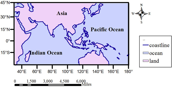
The study area AIPO lies between 30°S and 45°N, 30°E, and 180°E, as shown in Figure 1. The ocean–atmosphere interaction over AIPO has significant impacts on the short-term climate variations and predictions in China and surrounding areas (Wu et al., 2006; Li et al., 2013). Therefore, it is of vital importance to provide SST with high accuracy, high spatial completeness, and high spatiotemporal resolution in this region.
Data
This research uses two kinds of satellite-derived SSTs, that is, moderate-resolution imaging spectroradiometer (MODIS) SST, that is, IR SST, and advanced microwave scanning radiometer for EOS (AMSR-E) SST, that is, MW SST for merging, and drifting buoy observations as the ground truth for validation purpose, as illustrated in Table 1 and detailed in the following subsections.
MODIS SST
MODIS SST that is used in this research is the MODIS Aqua Global Level 3 Mapped Thermal SST products derived from the 11 and 12 µm thermal infrared bands, produced and distributed by the Ocean Biology Processing Group (OBPG) at the NASA GSFC (OBPG, 2015; Werdell et al., 2013). Daily, weekly, monthly, and annual MODIS products can be obtained at the spatial resolutions of both 4.63 and 9.26 km, and for both day and night passes. To avoid diurnal warming caused by solar heating of the ocean surface, and to provide high spatiotemporal resolution SST, the daily 4 km-resolution nighttime SST products at 1:30 am local time are chosen. The version of this dataset is v2014.0 released on August 31, 2015. The time span of this dataset is from July 4, 2002 to present, and in this study, the daily MODIS SST data in 2005 are chosen, with 363 images in total (the MODIS SST on November 17, 2005 and that on November 20, 2005 are excluded).
The SST data used are in the format of netCDF with two layers, including a temperature data layer and a data quality control layer. The data quality control layer has the same number of pixels as the temperature data layer, recording a quality label of the corresponding SST on the temperature data layer. The quality flags are as following: 0 represents good, 1 represents questionable, 2 represents clouds, and 255 represents gross clouds, land, and other errors. In this research, the MODIS SST pixels with the quality flag equaling 0 are used for the modeling process. The temperature data represent the temperature at the depth of a few micrometers, with a valid retrieval range of −2°C–32°C (Armstrong, 2007).
AMSR-E SST
AMSR-E SST is derived from the remote sensing data of AMSR-E on NASA’s EOS Aqua spacecraft, produced by Remote Sensing Systems (RSS), and sponsored by the NASA AMSR-E Science Team, and the NASA Earth Science MEaSUREs Program (Wentz et al., 2014). The data version is v7 released in October 2011. The daily SST products provided by RSS are orbital data that are mapped to 0.25°C grid, and divided into two maps based on ascending (1:30 pm) and descending (1:30 am) passes. To be consistent with the MODIS SST data in time, the data measured at 1:30 am are chosen.
The AMSR-E SST data are the temperature of the top layer of water, which is about 1 mm thick. The original data values are in the range of 0–255, with 0–250 indicating valid geophysical data, 251 indicating missing SST, 252 indicating sea ice, 253 indicating bad observations which are not used in composite maps, 254 indicating no observations, and 255 indicating land mass. The original data values have to be scaled to get meaningful SST, which is achieved by multiplying the scale factor (0.15) and adding the offset (−3.0) (RSS, 2021). Therefore, the valid value for AMSR-E SST is -3°C–34.5°C.
Drifting Buoy SST
Drifters are expendable satellite-tracked systems which drift in response to ocean currents and winds. Currently, there are more than 1,000 drifters circulating in the world ocean, measuring SST and other properties (e.g., atmospheric pressure, sea salinity, wind speed, and wind direction) at unprecedented resolution as ocean currents carry them along. The drifting buoy observations are usually used to correct the satellite measurement of ocean environmental parameters.
The drifting buoy SST data that are used in this research are collected, processed, and quality-controlled by the Atlantic Oceanographic and Meteorological Laboratory (AOML) (Lumpkin & Centurioni, 2019). The measurements are obtained at a depth of 0.2–0.3 m. The raw observations are interpolated into quarter-day intervals at 00:00, 06:00, 12:00, and 18:00 UTC using an optimal interpolation procedure. For the purpose of minimizing the possible diurnal warming of in situ SST and avoiding cold bias of the AMSR-E SST and MODIS SST, the minimum value of the observations of a day is chosen as daily ground truth for validation of the merged SST (Li et al., 2013; Tang et al., 2015). Before using the drifting buoy data, we remove the gross errors which are beyond the range of −1.8 °C–35 °C (Høyer et al., 2012). The chosen drifting buoy SST at the same day is then mapped to 4 km × 4 km grids for the MODIS SST and merged SST, and 25 km × 25 km grids for AMSR-E SST by averaging the drifting buoy data belonging to the same grid as the corresponding satellite SST.
Methods
The workflow of the method is depicted in Figure 2. First, ocean pixels are extracted in MODIS SST, based on AMSR-E SST. Then AMSR-E SST and MODIS SST pixels are matched based on locations, and quad-tuples (SSTAMSR-E, latitude, longitude, and SSTMODIS) are obtained. After preprocessing, including outlier removal and normalization, the quad-tuples are used by the genetic algorithm to obtain optimal initial parameters for the neural network model. Then the optimized neural network is trained with the quad-tuples to establish a mapping function between (SSTAMSR-E, latitude, and longitude) and SSTMODIS. The mapping function is later used to reconstruct the MODIS SST where MODIS SST is missing, but AMSR-E SST exists. The final merged SST is achieved by combining the reconstructed MODIS SST with the original MODIS SST and performing necessary post-processing. The following subsections detail the main steps of the method.
Extracting Ocean Pixels in MODIS SST Based on AMSR-E SST
Extracting ocean pixels from the satellite SST data is the prior step for further evaluating the spatial coverage of satellite SST before and after merging. It can be easily achieved for AMSR-E SST because the land pixels are marked separately in AMSR-E SST with a flag value 255. However, we cannot directly determine land pixels in MODIS SST because the MODIS SST quality control layer uses the same flag 255 to represent land, gross clouds, and other errors. By using the cross-check method proposed in the studies by Li et al. (2013) and Zhu et al. (2018), we can extract the land pixels in MODIS SST and further obtain the ocean pixels with the assistance of AMSR-E SST. The principle of this method is formulated as
Namely, for a pixel in MODIS SST flagged with 255 (potential land), if the AMSR-E SST pixel that spatially overlaps the most with the target MODIS pixel is marked as land, then the MODIS SST pixel is identified as land. Otherwise, it is regarded as an ocean pixel with gross clouds and other errors. When the land pixels are identified in MODIS SST, ocean pixels can then be easily extracted.
Data Location Matching
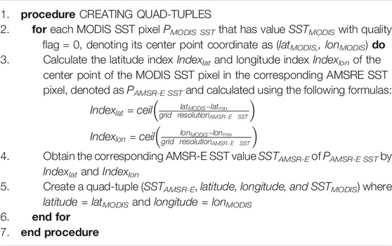
To achieve high-resolution and high-spatial-coverage merged SST, the missing high-resolution MODIS SST pixels should be reconstructed based on the low-resolution cloud-free AMSR-E SST, where the AMSR-E SST has value. Therefore, an important step of our method is establishing a mapping relation between the MODIS SST and AMSR-E SST at the same location. To achieve this, first we must match MODIS SST and AMSR-E SST where the values of both SST exist in the study area. The output of the matching is quad-tuples (SSTAMSR-E, latitude, longitude, and SSTMODIS), which will feed into the deep neural network model for model establishment. Algorithm 1 achieves this goal, where grid resolutionAMSR-E SST = 0.25°, and ceil(x) function rounds x to the smallest integer that is bigger than or equal to x.
Outlier Removal and Normalization
Before feeding the quad-tuples (SSTAMSR-E, latitude, longitude, and SSTMODIS) for model establishment, first we must perform some preprocessing for data quality control, including outlier removal and data normalization. The outlier removal can help avoid the decrease in modeling accuracy caused by outliers in the training data (Khamis et al., 2005). The normalization of the quad-tuples can enhance the neural network’s training speed and performance (Puheim & Madarász, 2014).
For outlier removal, we calculate the difference between AMSR-E SST and MODIS SST of each quad-tuple and obtain a difference value set. The quad-tuple with its difference value falling outside of 3 standard deviations of mean of the difference set are flagged as an outlier and removed. Then, the remaining quad-tuples go to the next step for normalization.
To perform normalization, we first split the N rows (N is the number of quad-tuples obtained after outlier removal) of quad-tuples (SSTAMSR-E, latitude, longitude, and SSTMODIS) into N rows of triple-tuples (SSTAMSR-E, latitude, and longitude) and N rows of scalar value SSTMODIS. Then, we map values of each row of both the triple-tuples and the scalar values to [-1 1] by using the following equation.
where
Genetic Algorithm–Assisted Deep Neural Network Model
Deep neural network models are good at modeling nonlinear and complex relationships among variables. Therefore, in this research, we use a deep neural network model for modeling the relationships between MODIS SST and AMSR-E SST together with locations, namely, obtaining the relationship
Deep Neural Network Model
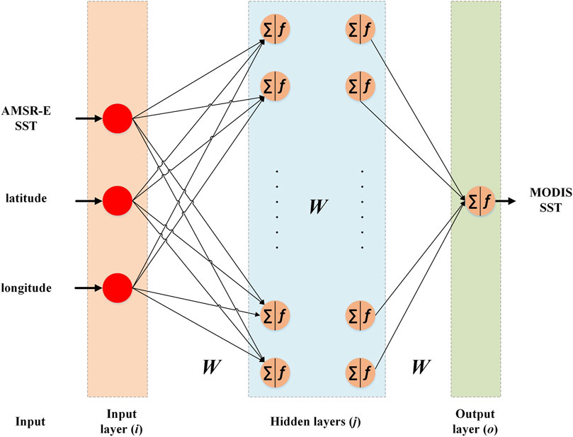
The deep neural network model used in this research is a feed-forward deep neural network model, the structure of which is shown in Figure 3. It consisted of an input layer, one or more hidden layers, and an output layer. Each layer is consisted of a number of neurons. Neurons between the layers are connected with varying weights (denoted as W in Figure 3). The weighted sum (denoted using the operator ∑ in Figure 3) of all the inputs to a neuron plus a bias is activated by an activation function f (·), producing the output of the neuron.
The deep neural network model is trained by using a backpropagation (BP) algorithm. The interconnecting weights and bias are updated iteratively to minimize the output error, which is usually a mean-square-error (MSE) between the targeted outputs and actual outputs of the neural network over all the training samples (Zare Abyaneh et al., 2016), and is calculated as
where b and w denote all the bias and weights in the network, respectively. N denotes the number of inputs, x is the input of the network, and
During the backpropagation, the weights and bias are updated using a gradient descent strategy. In each iteration, the gradient is first calculated using
Then, each weight and bias are updated using the increment,
where η is the learning rate, which is a constant.
The following parameters need to be determined in the deep neural network model: the number of hidden layers, the number of neurons in each hidden layer, the activation function for each layer, and the learning rate. The parameters in this study are set by combining experience and experiments. We choose a 3-layer architecture with three neurons for the input layer which receives the input triple-tuples (SSTAMSR-E, latitude, and longitude), seven neurons for the hidden layer, and one neuron for the output layer which outputs the estimated SSTMODIS value. The number of hidden layers and number of neurons in each hidden layer are determined by the process that we first chose several configurations of the number of hidden layers and the number of neurons in each hidden layer, then we compare the prediction performance of each configuration, and finally, the one that achieves the best performance is chosen. The sigmoid function is used as the activation function for the hidden layer, and the linear function is used as the activation function for the output layer. The learning rate is set to 0.05.
Genetic Algorithm–Based Deep Neural Network Parameter Optimization
By using the gradient descent method, the cost function is driven to a low value which however is without global convergence guarantee. Besides, the gradient-based training method is sensitive to the values of initial parameters (i.e., weights and bias). Thus, to prevent the deep neural network model from being trapped in a local minimum, the GA approach is adopted.
GA is a meta-heuristic method for solving optimization problems. Some researchers have demonstrated that GA can be used to help the neural network achieve global optimum (Mahmoudabadi et al., 2009; Wang et al., 2016; Yu & Xu, 2014). GA is based on the process of natural selection (Whitley et al., 1990), during which a population of individual solutions is repeatedly modified, and the population finally reaches an optimal solution through successive generations based on the following rules.
• Selection: select individuals as parents in the current generation to reproduce next generation based on their fitness.
• Crossover: combine the genes of parents to produce children as individuals in the next generation.
• Mutation: introduce random changes to a chromosome to produce children for the next generation.
Specifically, for optimizing the deep neural network model in this study, parameters of the neural network, including weights and bias (w, b), are encoded to a chromosome, and a population of such chromosomes is created and initialized. The fitness of each chromosome is evaluated using
where C(x,w,b) is the MSE of the deep neural network model whose parameters are specified by the chromosome. The L2 regularization term
There are several parameters in GA that need to be set, including initial population size, number of elite children (individuals with top fitness and directly selected to the next generation of population without any change), crossover fraction, and mutation rate. In this study, we set these parameters empirically, as listed in Table 2.
Performance Validation of the Model
Before applying the GA-DNNM to the merging AMSR-E SST and MODIS SST, the performance of the model should be first validated. In this study, we randomly select 90% of the normalized quad-tuples obtained in section Outlier Removal and Normalization to train the neural network and the remaining 10% to test the generalization performance of the trained network. Two indexes are utilized for performance evaluation: the mean error and root-mean-square-error (RMSE), which is defined as
where di is the error vector calculated by the difference between the desired MODIS SST value and the estimated MODIS SST value of the GA-DNNM, and n is the total number of test samples.
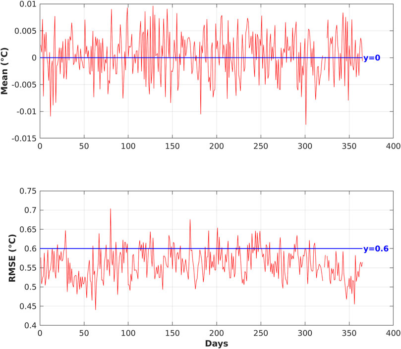
Performance validation results obtained during the experimental period are shown in Figure 5. From the testing results, the mean errors are almost equal to 0 °C, and 84.02% of the RMSEs are below 0.6°C. The estimated probability densities of the residuals of prediction on the test dataset of the first day of each month in 2005 are shown in Figure 6. It can be seen that the residuals are concentrated around 0. The validation results demonstrate a high generalized prediction accuracy of the GA-DNNM. Therefore, the GA-DNNM is capable of establishing the relationship between AMSR-E SST and MODIS SST through learning from the training dataset and can be further applied to merging these two SSTs.
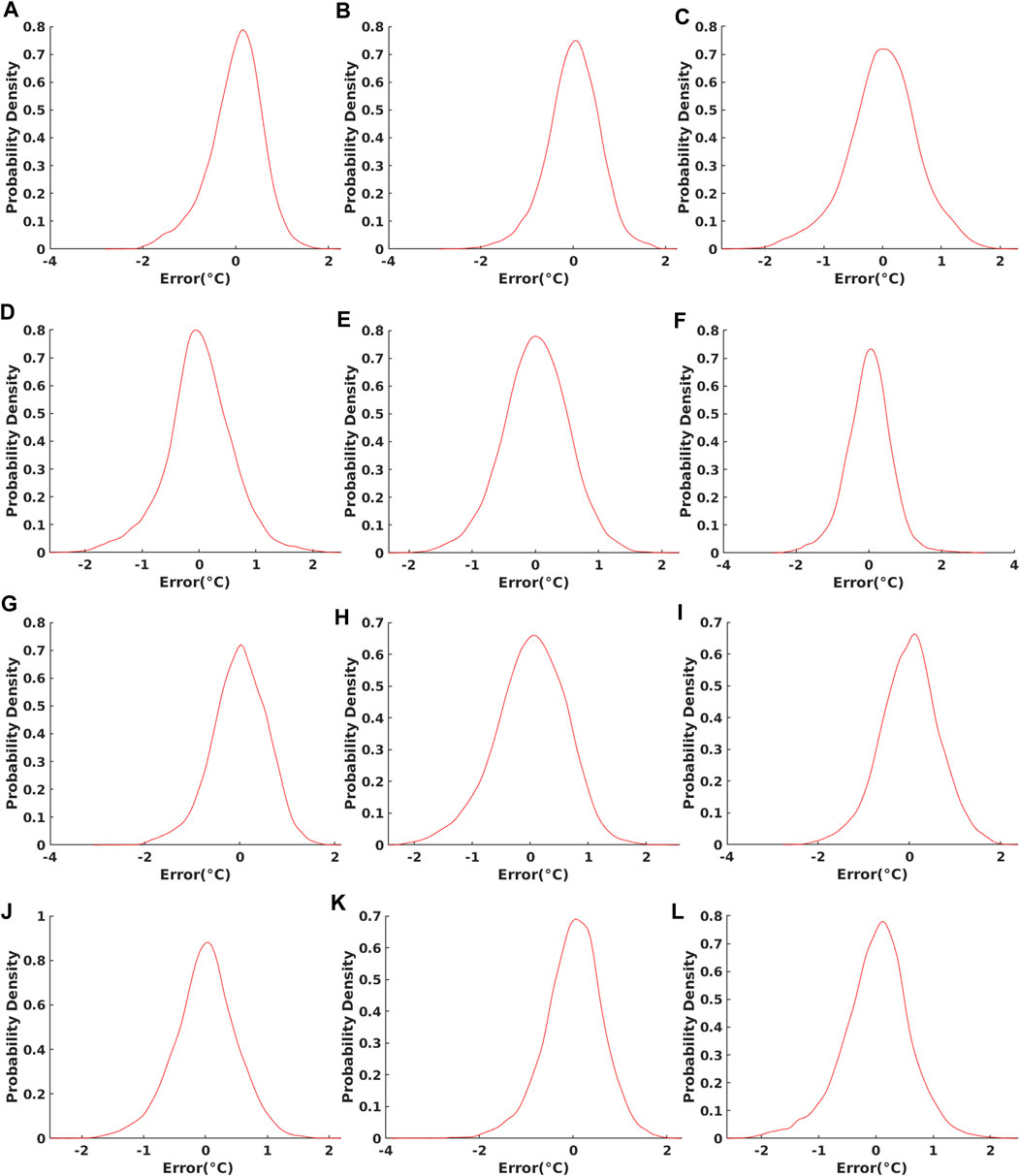
FIGURE 6. Estimated probability density of residuals of the proposed GA-DNNM for prediction on test data. Subfigures (A)–(L) are the estimated probability densities of residuals for the first day of January to December in 2005, respectively.
Post-Processing
When the merged SST has been obtained by GA-DNNM, we post-process it by removing pixels with gross error. The gross error pixels are those whose SST values are beyond the range of −3°C–35°C, which is the union of the valid data range of the MODIS SST and that of the AMSR-E SST.
Results and Discussion
For evaluating the proposed method, experiments are conducted on each day of 2005, expect for November 17, 2005 when the AMSR-E SST’s spatial coverage is 0.0% in the study area, and November 20, 2005 when the AMSR-E SST’s spatial coverage is 0.0524% in the study area and has no match with the drifting buoy observations. 4 km daily merged SST products with improved quality are generated in the AIPO area.
Comparison of the Spatial Coverage of MODIS SST, AMSR-E SST, and Merged SST
The spatial coverage is a critical index for measuring the quality of SST. In this section, we evaluate the spatial coverage of MODIS SST, AMSR-E SST, and merged SST both visually and quantitatively.
Intuitively, from Figure 7, we can see that the spatial coverage and continuity of SST are greatly improved after merging. The atmospheric contaminations and costal effects have been eliminated extensively. Further, in a quantitative way, we examine the spatial coverage of the three SSTs in the year 2005, in the study area using the following formula.
where Nvalid SST and Nocean denote the number of valid SST pixels and total ocean pixels, respectively. The number of ocean pixels is obtained using the method introduced in section Extracting Ocean Pixels in MODIS SST Based on AMSR-E SST.
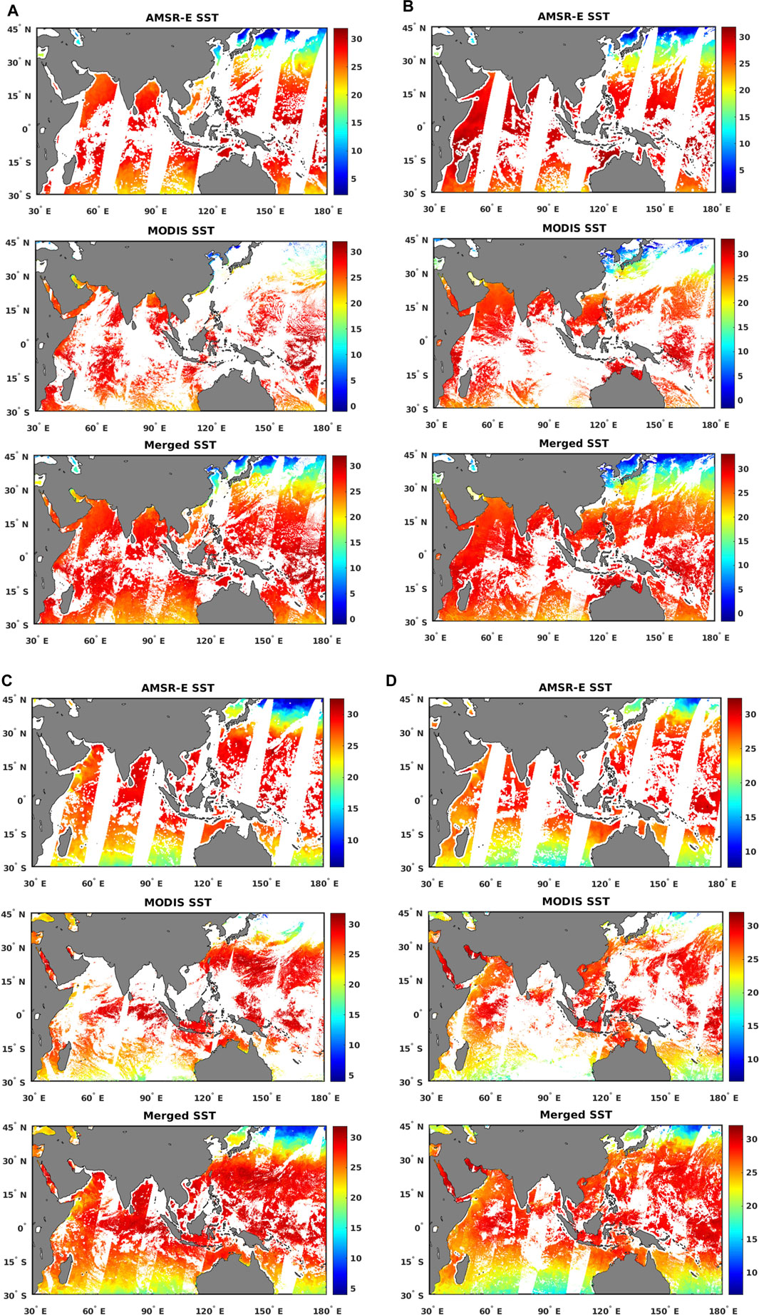
FIGURE 7. Spatial patterns of AMSR-E SST, MODIS SST, and merged SST on selected days in each season in 2005 with white color representing missing ocean pixels and gray color representing land pixels (A) from top to bottom: the three SSTs on January 1, 2005; (B) from top to bottom: the three SSTs on April 1, 2005; (C) from top to bottom: the three SSTs on July 1, 2005; and (D) from top to bottom: the three SSTs on October 1, 2005.
The quantitative results are shown in Figure 8. The spatial coverage of the original MODIS SST, original AMSR-E SST, and merged SST are ranging from 25.0 to 48.1%, 31.5 to 47.6%, and 56.1 to 73.1%, respectively. The merged SST has much higher spatial coverage than MODIS SST and AMSR-E SST, with a minimum improvement by 50.2% on April 19, 2005 and maximum improvement by 131.7% on December 9, 2005 compared with MODIS SST. The improvement of the spatial coverage relative to AMSR-E SST ranges from 32.3 to 79.2%. The spatial coverage of AMSR-E SST is quite stable, while there is more fluctuation for MODIS SST due to the vulnerability of the MODIS sensor to various atmospheric contaminations such as cloud cover, thick fogs, and concentrated aerosols. The spatial coverage of merged SST has the same fluctuation characteristics as MODIS SST because of the stability of AMSR-E SST and fluctuation of MODIS SST.
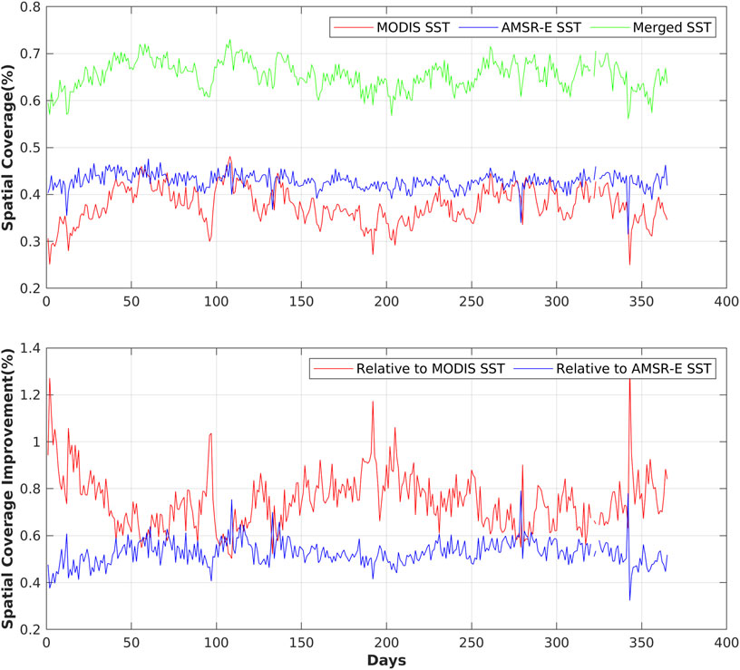
FIGURE 8. Comparison of spatial coverage of the daily MODIS SST, daily AMSR-E SST, and daily merged SST in 2005 in the AIPO area.
Validation of Reconstructed SST and Merged SST With Drifting Buoy Observations
To validate the reconstructed SST and merged SST (SST in the whole study area), a linear regression of the MODIS SST with the drifting buoy observations, the AMSR-E SST with the drifting buoy observations, the reconstructed SST with the drifting buoy observations, and the merged SST with the drifting buoy observations are performed each for each day in the study period. R-square (R2), RMSE, mean bias (Bias), and correlation coefficient are used for quantitatively evaluating the accuracy of SST.
To be concise, we select 1 day in each season to illustrate the accuracy of merged results, as shown in Figure 9A–D. From Figure 9, it can be seen that R2 and correlation coefficient of reconstructed SST are with little difference with those of AMSR-E SST but are much greater than those of MODIS SST. The RMSE of reconstructed SST in the time frame mostly lies between that of the AMSR-E SST and MODIS SST, that is, greater than AMSR-E SST and smaller than MODIS SST. The bias of the reconstructed SST is also much smaller than that of the MODIS SST. As with the finally merged SST, its R2 and correlation coefficient are greater than those of MODIS SST, and the RMSE greater than that of AMSR-E SST and reconstructed SST but smaller than that of MODIS SST. The reason why merged SST has bigger RMSE than reconstructed SST is that during the integration of reconstructed SST and MODIS SST to produce merged SST, the error of MODIS SST may be introduced. The RMSE and bias of the merged SST are acceptable, with higher accuracy than MODIS SST, and meanwhile keeps the same spatial resolution (4 km) and temporal resolution (1 day) as MODIS SST.
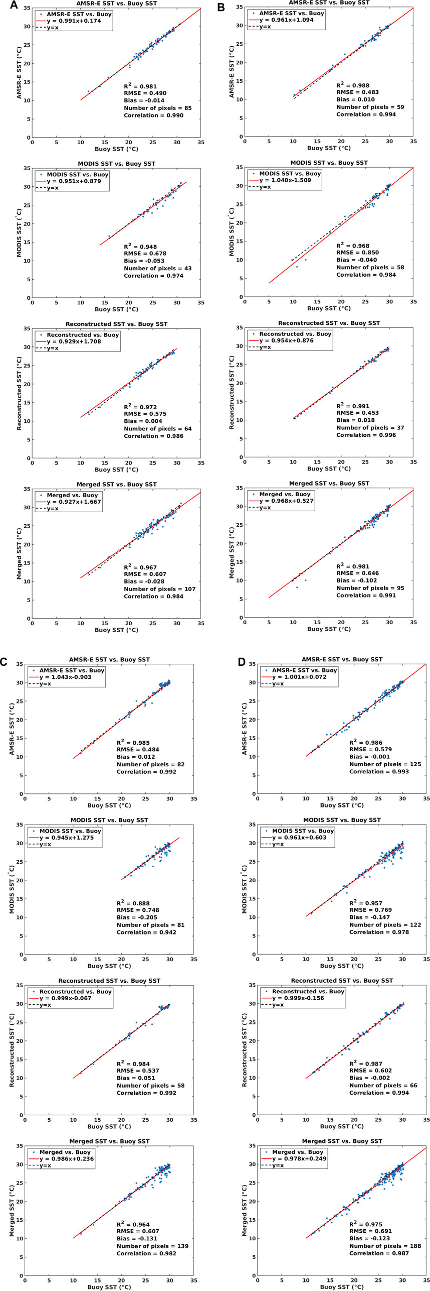
FIGURE 9. Validation of reconstructed SST and merged SST with drifting buoy observations on selected date in each season in 2005. From top to bottom: (A) validation on January 1, 2005, (B) validation on April 1, 2005, (C) validation on July 1, 2005, and (D) validation on October 1, 2005.
The average RMSE and average bias of the reconstructed SST are 0.502°C and 0.006°C, respectively. The average RMSE and average bias of the merged SST in the AIPO area are 0.603°C and −0.082°C, respectively. Errors of the merged SST may come from three aspects: 1) error of AMSR-E SST and MODIS SST: the merged SST is based on the AMSR-E SST and MODIS SST. Therefore, errors existing in two merging source of SST may contribute to errors in merged SST. 2) Errors of GA-DNNM can also be a source of errors for the merged SST; 3) difference of measured depth: AMSR-E SST, MODIS SST, and buoy SST measured at ∼ um (skin SST), ∼ 1 mm and 0.2–0.3 m (bulk SST), respectively. The merged SST can be seen measuring the same depth as MODIS SST, which however is coupled with the atmosphere–ocean exchange of heat and momentum closely, making the bulk-skin difference a quantity which varies with quite short time and space scales (Emery et al., 2001; Zhu et al., 2018).
Efficiency Analysis of the Proposed Method
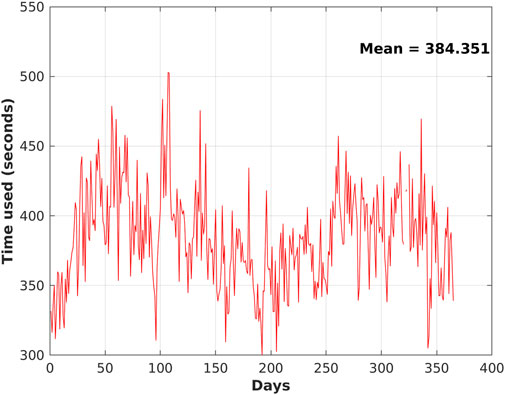
The time taken for the whole processing process each day, including data preprocessing, data location matching, GA-DNNM establishment, and SST merging, is shown in Figure 10. The time fluctuates for different days, with the longest time being 502.964 s on April 17 and the lowest time being 300.072 s on July 11, and the average time for each day being 384.351 s. It is little bit time-consuming, due to two reasons: 1) In the genetic algorithm, each chromosome carries 36 genes (calculated based on the structure of the neural network designed) that need to be optimized, and the number of inputs used for evaluating fitness of individuals in a population in each generation is firmly large (around 200,000–350,000) which involves lots of computation. 2) The procedure runs on a desktop with one Intel (R) Core (TM) i9-9,920X CPU at 3.5GHz and 48.0 GB RAM, whose computing resources and computing capabilities are limited. The fluctuating characteristics of the time consumed in each day are primarily because of the varying number of inputs for the genetic algorithm, neural network model training, and SST reconstruction. In future research, the configuration of the genetic algorithm may be further optimized, and high-performance computing (HPC) infrastructure and technologies (Wright and Wang, 2011) may be used to improve the efficiency.
Conclusions
SST is a crucial parameter for oceanic and atmospheric models. It plays an important role for weather forecasting and climate change monitoring. Therefore, getting high-resolution SST both in time and space, as well as high spatial coverage, is of vital importance. Satellite observations are the major sources based on which large-area SST is derived. However, due to the difference in the imaging mechanism, different satellite observations have different limitations. Infrared satellite sensors usually have high spatial resolutions but are vulnerable to various atmospheric contaminations such as cloud cover, thick fogs, and concentrated aerosols, while microwave sensors can penetrate clouds and aerosols but usually with low resolution and cannot obtain data near coasts. Consequently, a single sensor usually cannot achieve desirable SST.
This study therefore merges SST data from both infrared sensor (MODIS SST) and microwave sensor (AMSR-E SST) synergistically to produce daily SST with a spatial resolution of 4 km which has a much higher spatial coverage than the SST of each sensor, much higher spatial resolution than SST of microwave sensor, and higher accuracy than SST of infrared sensor. During this process, a genetic algorithm–assisted deep neural network model is established and evaluated. The validation of the reconstructed SST with drifting buoy observations each day during the year 2005 (363 days of data are analyzed) shows an average RMSE and average bias of 0.502°C and 0.006°C, respectively, and an average RMSE and average bias of 0.603°C and −0.082°C, respectively, for the merged SST in the whole study area. With the high generalized prediction accuracy, the model can be used for extended merging of the MODIS SST and AMSR-E SST in other years.
With the improved SST, extensive climate applications promise to be better supported, and the marine environment including spatiotemporal patterns and variability can be better monitored and understood than using SST from a single sensor alone. Furthermore, the method is applicable to merging SST at a global scale, which can provide improved data for and further benefit global and regional climate research and applications.
The GA-assisted optimization strategy is both computation- and data-intensive, which takes significant time for the GA-DNNM workflow. For future work on larger geographic areas, cyberGIS and high-performance computing approaches may be developed to accelerate and enhance the workflow (Liu & Wang, 2015; Wang & Goodchild, 2019). Besides, the proposed model currently could only be applied to the locations where AMSR-E SST is available, making it hard to achieve daily merged SST with 100% spatial coverage. How to expand the proposed model to incorporate more kinds of satellite-derived SSTs and drifting buoy observations to produce spatially seamless SST may also be a future direction.
Data Availability Statement
Publicly available datasets were analyzed in this study. These data can be found here: The MODIS SST data analyzed for this study can be obtained at PO. DACC website: https://podaac.jpl.nasa.gov/dataset/MODIS_AQUA_L3_SST_THERMAL_DAILY_4KM_NIGHTTIME_V2014.0. The AMSR-E SST analyzed for this study can be obtained at the Remote Sensing Systems website: http://data.remss.com/amsre/bmaps_v07/y2005/). The drifting buoy data analyzed for this study can be obtained at NOAA National Centers for Environmental Information website: https://doi.org/10.25921/7ntx-z961.
Author Contributions
CX, CH, and NC conceived and designed the experiments; CX performed the experiments; CX, ZC, and XZ analyzed the data; CX wrote the paper; and XT helped revise the paper.
Funding
This research was supported by the National Nature Science Foundation of China (NSFC) Program (Nos. 42001372 and 42071380), the National Key R&D Program (No. 2018YFB2100501), the Project funded by China Postdoctoral Science Foundation (Nos. 2019M661621 and 2021T140513), Shanghai Municipal Science and Technology Major Project (No. 2021SHZDZX0100), and Shanghai Municipal Commission of Science and Technology Project (No.19511132101).
Conflict of Interest
The authors declare that the research was conducted in the absence of any commercial or financial relationships that could be construed as a potential conflict of interest.
Publisher’s Note
All claims expressed in this article are solely those of the authors and do not necessarily represent those of their affiliated organizations, or those of the publisher, the editors, and the reviewers. Any product that may be evaluated in this article, or claim that may be made by its manufacturer, is not guaranteed or endorsed by the publisher.
Acknowledgments
The authors would like to thank the following data, tool, and service providers: OBPG at the NASA Goddard Space Flight Center and NASA Physical Oceanography Distributed Active Archive Center (PO.DACC) for providing MODIS SST data and corresponding data reading software; Remote Sensing Systems (RSS) for providing AMSR-E SST data and corresponding data reading routines (AMSR data are produced by Remote Sensing Systems and were sponsored by the NASA AMSR-E Science Team and the NASA Earth Science MEaSUREs Program. Data are available at www.remss.com); NOAA National Centers for Environmental Information for providing AOML Global Drifter interpolated data. The authors would also like to thank Professor Shaowen Wang at the University of Illinois at Urbana-Champaign for his help in the investigation of this work.
References
Armstrong, E. (2007). MODIS Sea Surface Temperature (SST) Products. Available at: ftp://podaac-ftp.jpl.nasa.gov/allData/modis/L3/docs/modis_sst.html (Accessed March 1, 2021).
Bretherton, F. P., Davis, R. E., and Fandry, C. B. (1976). A Technique for Objective Analysis and Design of Oceanographic Experiments Applied to MODE-73. Deep Sea Res. Oceanographic Abstr. 23 (7), 559–582. doi:10.1016/0011-7471(76)90001-2
Cai, Y., Guan, K., Peng, J., Wang, S., Seifert, C., Wardlow, B., et al. (2018). A High-Performance and In-Season Classification System of Field-Level Crop Types Using Time-Series Landsat Data and a Machine Learning Approach. Remote Sensing Environ. 210, 35–47. doi:10.1016/j.rse.2018.02.045
Chang-Xiang, Y., Jiang, Z., and Ji-Ping, X. (2010). An Ocean Reanalysis System for the Joining Area of Asia and Indian-Pacific Ocean. Atmos. Oceanic Sci. Lett. 3 (2), 81–86. doi:10.1080/16742834.2010.11446848
Chao, Y., Li, Z., Farrara, J. D., and Hung, P. (2009). Blending Sea Surface Temperatures from Multiple Satellites and In Situ Observations for Coastal Oceans. J. Atmos. Ocean. Technol. 26 (7), 1415–1426. doi:10.1175/2009JTECHO592.1
Dahl, G. E., Dong Yu, D., Li Deng, L., and Acero, A. (2012). Context-Dependent Pre-trained Deep Neural Networks for Large-Vocabulary Speech Recognition. IEEE Trans. Audio Speech Lang. Process. 20 (1), 30–42. doi:10.1109/TASL.2011.2134090
Donlon, C. J., Martin, M., Stark, J., Roberts-Jones, J., Fiedler, E., and Wimmer, W. (2012). The Operational Sea Surface Temperature and Sea Ice Analysis (OSTIA) System. Remote Sensing Environ. 116, 140–158. doi:10.1016/j.rse.2010.10.017
Emery, W. J., Castro, S., Wick, G. A., Schluessel, P., and Donlon, C. (2001). Estimating Sea Surface Temperature from Infrared Satellite and In Situ Temperature Data. Bull. Amer. Meteorol. Soc. 82 (12), 2773–2785. doi:10.1175/1520-0477(2001)082<2773:ESSTFI>2.3.CO;2
Guan, L., and Kawamura, H. (2004). Merging Satellite Infrared and Microwave SSTs: Methodology and Evaluation of the New SST. J. Oceanogr. 60 (5), 905–912. doi:10.1007/s10872-005-5782-5
Guo, P. (2010). “Study on Bayesian Hierarchal Model-Based SST Data Fusion Methods,” in Proc. Remote Sensing of the Ocean, Sea Ice, and Large Water Regions 2010. Editors R. B. Charles, P. M. Stelios, N. Xavier, and V.-R. Miguel (Washington, United States: International Society for Optics and Photonics), 7825O. doi:10.1117/12.864912
Høyer, J. L., Karagali, I., Dybkjær, G., and Tonboe, R. (2012). Multi Sensor Validation and Error Characteristics of Arctic Satellite Sea Surface Temperature Observations. Remote Sensing Environ. 121, 335–346. doi:10.1016/j.rse.2012.01.013
Kaul, M., Hill, R. L., and Walthall, C. (2005). Artificial Neural Networks for Corn and Soybean Yield Prediction. Agric. Syst. 85 (1), 1–18. doi:10.1016/j.agsy.2004.07.009
Khamis, A., Ismail, Z. I., Khalid, K. H., and Mohammed, A. T. (2005). The Effects of Outliers Data on Neural Network Performance. J. Appl. Sci. 5 (8), 1394–1398. doi:10.3923/jas.2005.1394.1398
Le, T. H. (2011). Applying Artificial Neural Networks for Face Recognition. Adv. Artif. Neural Syst. 2011, 1–16. doi:10.1155/2011/673016
Li, A., Bo, Y., Zhu, Y., Guo, P., Bi, J., and He, Y. (2013). Blending Multi-Resolution Satellite Sea Surface Temperature (SST) Products Using Bayesian Maximum Entropy Method. Remote Sensing Environ. 135, 52–63. doi:10.1016/j.rse.2013.03.021
Li, T., Shen, H., Yuan, Q., Zhang, X., and Zhang, L. (2017). Estimating Ground-Level PM2.5 by Fusing Satellite and Station Observations: A Geo-Intelligent Deep Learning Approach. Geophys. Res. Lett. 44 (23), 11985–11993. doi:10.1002/2017GL075710
Liu, Y. Y., and Wang, S. (2015). A Scalable Parallel Genetic Algorithm for the Generalized Assignment Problem. Parallel Comput. 46, 98–119. doi:10.1016/j.parco.2014.04.008
Lumpkin, R., and Centurioni, L. (2019). Data from: Global Drifter Program Quality-Controlled 6-hour Interpolated Data from Ocean Surface Drifting Buoys. NOAA National Centers for Environmental Information. doi:10.25921/7ntx-z961
Mahmoudabadi, H., Izadi, M., and Menhaj, M. B. (2009). A Hybrid Method for Grade Estimation Using Genetic Algorithm and Neural Networks. Comput. Geosci. 13 (1), 91–101. doi:10.1007/s10596-008-9107-9
McIntosh, P. C. (1990). Oceanographic Data Interpolation: Objective Analysis and Splines. J. Geophys. Res. 95 (C8), 13529–13541. doi:10.1029/JC095iC08p13529
OBPG (2015). Data from: MODIS Aqua Level 3 SST Thermal IR Daily 4km Nighttime v2014.0. OBPG, v2014.0. CA, USA: PO.DAAC. doi:10.5067/MODSA-1D4N4
Panda, S. S., Ames, D. P., and Panigrahi, S. (2010). Application of Vegetation Indices for Agricultural Crop Yield Prediction Using Neural Network Techniques. Remote Sensing 2 (3), 673–696. doi:10.3390/rs2030673
Puheim, M., and Madarász, L. (2014). “Normalization of Inputs and Outputs of Neural Network Based Robotic Arm Controller in Role of Inverse Kinematic Model,” in Article Presented at 12th International Symposium on Applied Machine Intelligence and Informatics (Sami), IEEE, Herl'any, Slovakia (IEEE). doi:10.1109/SAMI.2014.6822439
Reynolds, R. W., Rayner, N. A., Smith, T. M., Stokes, D. C., and Wang, W. (2002). An Improved In Situ and Satellite SST Analysis for Climate. J. Clim. 15 (13), 1609–1625. doi:10.1175/1520-0442(2002)015<1609:AIISAS>2.0.CO;2
Reynolds, R. W., and Smith, T. M. (1995). A High-Resolution Global Sea Surface Temperature Climatology. J. Clim. 8 (6), 1571–1583. doi:10.1175/1520-0442(1995)008<1571:AHRGSS>2.0.CO;2
RSS (2021). AMSR-2/AMSR-E. Available at: http://www.remss.com/missions/amsr/(Accessed March 1, 2021).
Sexton, R. S., Dorsey, R. E., and Johnson, J. D. (1998). Toward Global Optimization of Neural Networks: A Comparison of the Genetic Algorithm and Backpropagation. Decis. Support Syst. 22 (2), 171–185. doi:10.1016/S0167-9236(97)00040-7
Tahmasebi, P., and Hezarkhani, A. (2012). A Hybrid Neural Networks-Fuzzy Logic-Genetic Algorithm for Grade Estimation. Comput. Geosciences 42, 18–27. doi:10.1016/j.cageo.2012.02.004
Tang, S., Yang, X., Dong, D., and Li, Z. (2015). Merging Daily Sea Surface Temperature Data from Multiple Satellites Using a Bayesian Maximum Entropy Method. Front. Earth Sci. 9 (4), 722–731. doi:10.1007/s11707-015-0538-z
USEPA (2021). Climate Change Indicators: Sea Surface Temperature. Available at: https://www.epa.gov/climate-indicators/climate-change-indicators-sea-surface-temperature (Accessed May 28, 2021).
Valverde Ramírez, M. C., de Campos Velho, H. F., and Ferreira, N. J. (2005). Artificial Neural Network Technique for Rainfall Forecasting Applied to the São Paulo Region. J. Hydrol. 301 (1-4), 146–162. doi:10.1016/j.jhydrol.2004.06.028
Wang, S., and Goodchild, M. F. (2019). CyberGIS for Geospatial Innovation and Discovery. Dordrecht, Netherlands: Springer. doi:10.1007/978-94-024-1531-5
Wang, S., Zhang, N., Wu, L., and Wang, Y. (2016). Wind Speed Forecasting Based on the Hybrid Ensemble Empirical Mode Decomposition and GA-BP Neural Network Method. Renew. Energ. 94, 629–636. doi:10.1016/j.renene.2016.03.103
Wang, W., and Xie, P. (2007). A Multiplatform-Merged (MPM) SST Analysis. J. Clim. 20 (9), 1662–1679. doi:10.1175/JCLI4097.1
Wright, D., and Wang, S. (2011). The Emergence of Spatial Cyberinfrastructure. PNAS 108 (14), 5488–5491. doi:10.1073/pnas.1103051108
Wentz, F. J., Gentemann, C., Smith, D., and Chelton, D. (2000). Satellite Measurements of Sea Surface Temperature through Clouds. Science 288 (5467), 847–850. doi:10.1126/science.288.5467.847
Wentz, F. J., Meissner, T., Gentemann, C., and Brewer, M. (2014). Data from: Remote Sensing Systems AQUA AMSR-E Daily Environmental Suite on 0.25 Deg Grid. R.S. System, V7. Santa Rosa, CA: Remote Sensing Systems. Available at: http://www.remss.com/missions/amsr/.
Werdell, P. J., Franz, B. A., Bailey, S. W., Feldman, G. C., Boss, E., Brando, V. E., et al. (2013). Generalized Ocean Color Inversion Model for Retrieving marine Inherent Optical Properties. Appl. Opt. 52 (10), 2019–2037. doi:10.1364/AO.52.002019
Whitley, D., Starkweather, T., and Bogart, C. (1990). Genetic Algorithms and Neural Networks: Optimizing Connections and Connectivity. Parallel Comput. 14 (3), 347–361. doi:10.1016/0167-8191(90)90086-O
Wu, G., Li, J., Zhou, T., Lu, R., Yu, Y., Zhu, J., et al. (2006). The Key Region Affecting the Short-Term Climate Variations in China: the Joining Area of Asia and Indian-Pacific Ocean. Adv. Earth Sci. 21 (11), 1109–1118. doi:10.11867/j.issn.1001-8166.2006.11.1109
Wu, W., Qiu, Z., Zhao, M., Huang, Q., and Lei, Y. (2018). Visible and Infrared Image Fusion Using NSST and Deep Boltzmann Machine. Optik 157, 334–342. doi:10.1016/j.ijleo.2017.11.087
Xiao, C., Chen, N., Hu, C., Wang, K., Gong, J., and Chen, Z. (2019). Short and Mid-term Sea Surface Temperature Prediction Using Time-Series Satellite Data and LSTM-AdaBoost Combination Approach. Remote Sensing Environ. 233, 111358. doi:10.1016/j.rse.2019.111358
Yu, F., and Xu, X. (2014). A Short-Term Load Forecasting Model of Natural Gas Based on Optimized Genetic Algorithm and Improved BP Neural Network. Appl. Energ. 134, 102–113. doi:10.1016/j.apenergy.2014.07.104
Yue, L., Shen, H., Zhang, L., Zheng, X., Zhang, F., and Yuan, Q. (2017). High-quality Seamless DEM Generation Blending SRTM-1, ASTER GDEM V2 and ICESat/GLAS Observations. ISPRS J. Photogrammetry Remote Sensing 123, 20–34. doi:10.1016/j.isprsjprs.2016.11.002
Zare Abyaneh, H., Bayat Varkeshi, M., Golmohammadi, G., and Mohammadi, K. (2016). Soil Temperature Estimation Using an Artificial Neural Network and Co-active Neuro-Fuzzy Inference System in Two Different Climates. Arab. J. Geosci. 9 (5), 377. doi:10.1007/s12517-016-2388-8
Zhang, X., and Chen, N. (2016). Reconstruction of GF-1 Soil Moisture Observation Based on Satellite and In Situ Sensor Collaboration under Full Cloud Contamination. IEEE Trans. Geosci. Remote Sensing 54 (9), 5185–5202. doi:10.1109/TGRS.2016.2558109
Keywords: sea surface temperature (SST), AMSR-E SST, MODIS SST, data fusion, genetic algorithm, deep neural network model
Citation: Xiao C, Hu C, Chen N, Zhang X, Chen Z and Tong X (2021) A Genetic Algorithm–Assisted Deep Neural Network Model for Merging Microwave and Infrared Daily Sea Surface Temperature Products. Front. Environ. Sci. 9:748913. doi: 10.3389/fenvs.2021.748913
Received: 28 July 2021; Accepted: 09 September 2021;
Published: 27 October 2021.
Edited by:
Peng Liu, Institute of Remote Sensing and Digital Earth (CAS), ChinaReviewed by:
Lei Guan, Ocean University of China, ChinaZenghong Liu, Ministry of Natural Resources, China
Manoj Singh, University of Petroleum and Energy Studies, India
Copyright © 2021 Xiao, Hu, Chen, Zhang, Chen and Tong. This is an open-access article distributed under the terms of the Creative Commons Attribution License (CC BY). The use, distribution or reproduction in other forums is permitted, provided the original author(s) and the copyright owner(s) are credited and that the original publication in this journal is cited, in accordance with accepted academic practice. No use, distribution or reproduction is permitted which does not comply with these terms.
*Correspondence: Chuli Hu, aHVjaGxAY3VnLmVkdS5jbg==
 Changjiang Xiao
 Chuli Hu3,4*
 Zeqiang Chen