 Chinmay Mallik
 Harish Gadhavi
 Shyam Lal
 Rahul Kant Yadav
 R. Boopathy
 Trupti Das
94% of researchers rate our articles as excellent or good
Learn more about the work of our research integrity team to safeguard the quality of each article we publish.
Find out more
ORIGINAL RESEARCH article
Front. Environ. Sci., 13 October 2021
Sec. Atmosphere and Climate
Volume 9 - 2021 | https://doi.org/10.3389/fenvs.2021.743894
This article is part of the Research TopicImpact of the COVID-19 Lockdown on the AtmosphereView all 10 articles
The COVID-19 pandemic resulted in changed emission regimes all over the world. India also imposed complete lockdown on all modes of travel and industrial activities for about 2 months from 25-March-2020 and later unlocked these activities in a phased manner. Here, we study signatures of emissions changes on levels of atmospheric trace gases and aerosols contributing to air pollution over multiple sites in India’s capital Delhi covering various lockdown and unlock phases using satellite data and in-situ observations. The resulting changes in the levels of these species were compared with respect to their average of 2015–2019 to attribute for year to year and seasonal changes. A clear impact of lockdown was observed for AOD, PM, NO2, CO, and SO2 as a result of emission changes, while changed precursor levels led to a change in O3 chemical regimes impacting its concentrations. A detailed analysis of FLEXPART trajectories revealed increased PM levels over Delhi in north-westerly air masses sourced to Punjab region all the way up to Pakistan. Changes in aerosols and NO2 were not only restricted to the surface but transcended the total tropospheric column. The maximum decrease in PM, NO2, CO, and SO2 was observed during the month of total lockdown in April. The lockdown impact varied with species e.g., PM10 and PM2.5 as well as locations even within the periphery of Delhi. While surface level aerosols and NO2 showed significant and almost similar changes, AOD showed much lower decrease than tropospheric column NO2.
Delhi is known for its high levels of air pollution with increasing emissions from various anthropogenic sources. Apart from local, anthropogenic emissions, Delhi’s air quality is also impacted by transport of pollutants from the nearby industrial and agricultural sources. Transport of pollutants from the agriculture residue burning both toward the end of autumn and spring in the nearby states of Punjab and Haryana is a regular feature every year. Planning effective strategies for controlling the levels of pollutants needs accurate emission inventories of various sources. The COVID-19 pandemic in India is part of the worldwide pandemic of coronavirus disease 2019 (COVID-19) caused by severe acute respiratory syndrome coronavirus 2 (SARS-CoV-2). The COVID-19 containment effort such as countrywide lockdown provided a unique opportunity to study how pollutant levels change in an otherwise highly polluted urban atmosphere following a curb in various anthropogenic emission sources. While this pandemic started in November 2019 in China, India saw the first case of COVID-19 on January 30, 2020 and the first reported death on March 12 (Andrews et al., 2020; 1). Henceforth, the infection rate continued to increase. A single-day trial lockdown was announced in India on March 22, followed by the first phase from March 25 and later various other phases for lockdown followed by phasewise unlock as detailed in Table 1 2,3. There are various studies related to the impact of lockdown on pollutant levels in different parts of the world (Le et al., 2020; Sicard et al., 2020; Xu et al., 2020) as well as in India (Dhaka et al., 2020; Jain and Sharma 2020; Mahato et al., 2020; Singh et al., 2020; Nath et al., 2021; Panda et al., 2021). Although this was a nationwide lockdown but we chose to study the impact over Delhi as it is the most polluted major urban region in India. This article provides a detailed account of the changes until almost the end of the government-enforced planned lockdown/unlock periods in 2020 and with respect to emission sources and lifetimes using surface-based in situ measurements as well as satellite-based measurements.
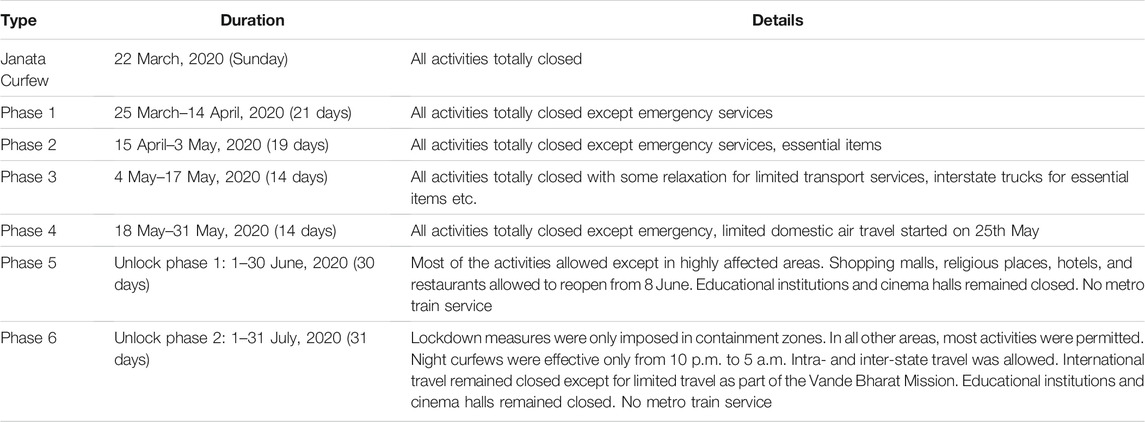
TABLE 1. Various phases of lockdown in India to arrest the spread of the infection due to COVID-19.
For the present analysis, we have focused on the Delhi metropolitan region (28.20–28.71°N, 77.17–77.38°E). The reasons are that Delhi is a megacity and home to a population of 29 million estimated in 2018 and projected to be the world’s most populous in a decade4,5. With an area of approximately 1,500 square kilometers, a population density of approximately 19,400 per square km, and being the capital city of India, Delhi is also a hub of connection with close to 11 million vehicles daily plying the roads of Delhi with a growth rate of 5% in 20186,7. Apart from that, Delhi also witnesses a significant flux of industrial emissions including the power plants. The Delhi-Mumbai industrial corridor is one of the biggest in the world. Additionally, a significant amount of pollution in Delhi is attributed to adjoining agriculture waste burning emissions (Perrino et al., 2011; Rajput et al., 2014). Emissions and air pollution were also found to impact the vertical temperature structure over Delhi, leading to accelerated warming (Mallik and Lal, 2011). So, when the COVID-19 was announced and the entire functioning transport system came to a halt suddenly, the impacts were expected to be significant. To understand the impact of lockdown on the emissions and the subsequent impact of these changed emissions as a result of enforcement of various lockdown/unlock phases on atmospheric concentrations of particulate matter (PM: 10 and 2.5), nitrogen dioxide (NO2), ozone (O3), cabon monoxide (CO), and sulphur dioxide (SO2), we have analyzed the respective data from six different locations in Delhi. These locations are given in Table 2 and are also shown in Figure 1. The study sites are: Anand Vihar (AnVh), Punjabi Bagh (PnBg), Shadipur (SdPr), Central Road Research Institute (CRRI), NSIT Dwarka (NstD), and EPA/US Embassy Delhi (EPA-D).
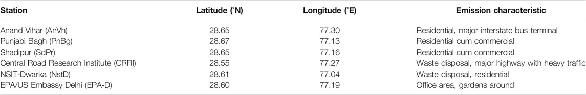
TABLE 2. Location and characteristics of sites chosen for this study.
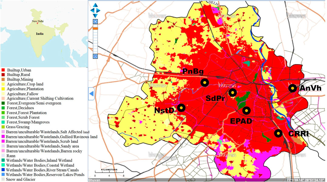
FIGURE 1. Map of Delhi showing the study locations. The Land Use Land Cover (LULC) map is downloaded from Bhuvan(https://bhuvan-app1.nrsc.gov.in/thematic/thematic/index.php). The study sites are: Anand Vihar (AnVh), Punjabi Bagh (PnBg), Shadipur (SdPr), Central Road Research Institute (CRRI), NSIT-Dwarka (NstD), and EPA/US Embassy Delhi (EPA-D).
Anand Vihar is a posh locality in the Eastern part of Delhi with many residential colonies and shopping complexes. It harbors a major railway station and is situated in the east of the River Yamuna. The major emission sources in this region are likely to be the residential and traffic sectors. However, in the western part, there are a few industries manufacturing paper, glass, and chemicals. While paper industries can be a secondary source of SO2, petrol pumps (and vehicles plying) in the region can be a significant source of hydrocarbons and NOx impacting local O3 chemistry.
The Central Road Research Institute is housed in a green campus in south east Delhi, just 1 km west of the Okhla Bird sanctuary on Mathura Road. Despite being in a green area, the measurements here would be significantly affected by sulfur and hydrocarbon emissions from landfill, with the Okhla Disposable Area of Delhi being in the immediate eastern neighborhood. The area also has several industries related to waste and garbage management. The area is surrounded by large educational hubs with IIT Delhi in the south-west and Jamia Millia Islamia in the north-east. There are a few hospitals toward the north, while industrial parks are located to the south.
The US Embassy is located in the very green and planned Chanakyapuri area of New Delhi surrounded by parks and other tourist attractions. The Rashtrapati Bhavan is less than 1 km to the north, Central Ridge Reserve Forest to the west, office/market/religious areas to the south, and Safdarjung Airport to the east. The major local emissions in this area are likely to be from the transport sector, mostly light motor vehicles. Shadipur and Punjabi Bagh are located less than 2 km apart in Central West Delhi and can be characterized as residential cum commercial area. Additionally, the Naraina Industrial Area lies 1 km south of Shadipur, while the Mangolpuri Industrial Area and Ordinance Depot (Shakurbasti) lie north of Punjabi Bagh, so both these areas are likely to be impacted by mixed emission regimes. Netaji Subhas University of Technology, Dwarka (NstD, henceforth NSIT-Dwarka) is located in the western part of Delhi in the vicinity of Indira Gandhi International Airport, the later lying to the east of the monitoring station in the educational institute. About 6 km to the north is situated the Scion Waste Water treatment plant. The Keshopur Sewage Treatment Plant is also in close vicinity.
The National Centres for Environmental Prediction (NCEP) Final (NCEP FNL) operational global analysis data are produced at 1° × 1° grid horizontally and 26 pressure levels vertically every 6 h using Global Data Assimilation System (GDAS). The GDAS assimilates all the observations such that the model produced gridded values are consistent with observations. For all practical purposes the reanalysis data are proxy for observations. The same data-set was also used to run the FLEXPART model described later. Figure 2 shows the 24 h average values of meteorology over New Delhi using NCEP FNL reanalysis data (National Centers for Environmental Prediction (NCEP)/National Weather Service/NOAA/U.S. Department of Commerce, 2000). The red dots show the daily 5 year (2015–2019) average of the value on a given day along with standard deviation whereas blue dots show the daily average of 2020. Five year mean values of temperatures steadily rose from March to mid-May and then started decreasing. The temperature in 2020 followed nearly the same trend as 5 year mean but in about three instances that were around day numbers 85, 110, and 150, a sudden decrease in temperature for a few days was observed. Corresponding to each of these three events, an increase in Relative Humidity (RH) and wind speed was observed. Overall, RH follows an inverse pattern of temperature variation and there is no systematic seasonal variation in wind speed. The planetary boundary layer height is low in March. It rises steadily in April and then remains high till the middle of June. Subsequently, it decreases but rather slowly.
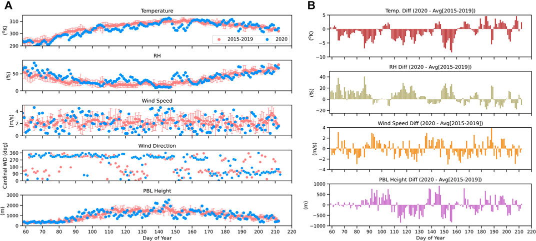
FIGURE 2. (A) Variations in daily average meteorological parameters during COVID-19 lockdown and unlock phases and comparison with daily 5-year average for the years 2015–2019. (B) Difference plot for meteorological parameters.
The Central Pollution Control Board (CPCB) monitors ambient air quality across stations spanning the entire Indian region with the help of the State Pollution Control Boards and other agencies under the National Air Quality Monitoring Programme (NAMP). Under NAMP, four air pollutants, viz. SO2, oxides of nitrogen as NO2, suspended particulate matter, and respirable suspended particulate matter, were identified for regular monitoring8. Along with it, measurements of O3 and CO are also available for many stations. PM measurements include PM2.5 and PM10. The suite of instruments constitutes a Continuous Ambient Air Quality Monitoring (CAAQM) station. Currently, monitoring is carried out over 233 CAAQM stations, mostly representing urban and industrial locations. In most cases, the monitoring data is available on an hourly basis. The data can be downloaded from the CPCB portal9. A major objective of CBCB for making these measurements is to present the Air Quality Indices (AQI)10. The AQI are used for resource allocation, enforcement of standards, to determine evolution (improvement/degradation) of air quality, to raise public awareness using simple infographics, and of course to help in scientific research. For this study, CAAQM station data were downloaded for 6 sites in Delhi as described in The Study Locations. The parameters considered for this study are PM10, PM2.5, NO2, O3, CO, and SO2.
The ultraviolet photometric O3 gas analyzers work on the standard principle of absorption of radiation at 254.7 nm by atmospheric O3. The lower detection limit of the instrument is 1 ppb with a response time of 30 s or less. The CO instruments are based on gas filter correlation technology and operate on the principle of infrared absorption at 4.67 μm vibration-rotation band of CO (Nedelec et al., 2003). It has a lower detection limit of 100 ppbv at a 60 s response time. The zero noise of the instrument is 20 ppbv root-mean-square (RMS) at 30 s averaging time. The NOx instruments are based on the detection of chemiluminescence produced by the oxidation of nitric oxide (NO) by O3 molecules, which peak at 630 nm radiation (Navas et al., 1997). The method is specific to NO only. NO2 is measured by converting it into NO using a molybdenum convertor and then measuring total NOx as NO. Unfortunately, the reduction of NO2 to NO is not specific for NO2, and other nitrogen species are also reduced to NO and act as interferences in the NO2 measurements. The lower detection limits of these instruments are approximately 1 ppb at a response time of 120 s or less. The SO2 measurements are based on UV fluorescence wherein SO2 is excited using 214 nm and a band pass filter centered approximately 350 nm is used to collect the fluorescence (Mallik et al., 2016). The PM10 measurements are based on the principle of β-ray attenuation. The particulate matter in ambient air is sampled through the instrument at a flow rate of 16 liters per minute and collected on fiberglass filter tape. Comparison of measurements of β-ray radiation by scintillation/G.M. counter before and after sampling gives a measure of the amount of PM10. The PM2.5 measurements are similar to PM10 but the particle size cutoff is in the range of 0–2.5 μm. The instrument specifications for obtaining these measurements can be found in the CPCB website8.
We have used daily average data for 5 selected sites from January, 2015 to July, 2020. However, there are data gaps for various species e.g. data for Central Road Research Institute are only available from the last quarter of 2017 (except availability of intermittent data in 2015: Jan–Apr, Sep–Nov), while data from Anand Vihar are missing during Jun–Oct 2017. Similarly data from Punjabi Bagh are missing from Nov 2016 to Oct 2017, while data from Shadipur is missing during Apr–Sep 2017. PM data of NSIT-Dwarka is missing during Dec 2015–Sep 2017.
Ozone Monitoring Instrument (OMI) is a spectrometer on board NASA EOS Aura satellite in sun-synchronous orbit with local equator crossing time 13:45 ± 0:15 h (Levelt et al., 2006). The spectrometer has a field of view 13 km × 24 km near nadir and 24 km × 160 km at the edges of swath. It has three channels—two in UV wavelength range and one in visible wavelength range with subnanometer spectral resolution. Columnar NO2 concentrations are estimated using visible channel radiance values in wavelength range 405–465 using the algorithm described in Lamsal et al. (2020). The NO2 spatial maps (0.25° × 0.25°) are made using cloud screened L3 data (Version 3) from OMI obtained through Giovanni iterface11. For the rest of the calculations and plots in this work, Version 4 OMI NO2 standard product (Krotkov et al., 2019) is used. The version 4 update includes use of field of view specific geometry dependent Lambertian surface reflectivity in NO2 retrieval and more accurate terrain pressure among several other improvements and has uncertainty less than 30%.
Visible Infrared Imager-Radiometer Suite (VIIRS) is a whiskbroom radiometer with 22 channels ranging from 0.41 to 12.01 µm on board Suomi National Polar-orbiting Partnership (NPP) satellite platform that was launched in October 2011. The VIIRS sensor is designed to extend and improve upon its predecessor namely MODIS and AVHRR. There are two different algorithms to estimate aerosol optical depth (AOD) (Levy et al., 2015; Sawyer et al., 2020). In this work, AOD estimated using the dark target algorithm is used (Levy et al., 2020)12.
FLEXPART (FLEXible PARTicle dispersion model) is an open-source Lagrangian particle dispersion model. The FLEXPART model can be run in forward or backward mode using user-supplied meteorological fields and allows for physical processes such as dry deposition, wet deposition, diffusion, convective transport, etc. to estimate dispersion or source-receptor relationships (Seibert and Frank, 2004; Pisso et al., 2019). The latest version 10.4 was run in backward mode to calculate source-receptor relationship for Delhi for each day starting from 15 January to 31 July in the current work. The source-receptor relationship is the sensitivity to the emissions located at a given grid-box for the receptor location. It represents the normalized total time spent by the back-trajectories in a given grid-box. We used 50000 trajectories spread over 24 h to estimate source receptor relationship for each day. A few source-receptor relationships for the grid-boxes close to the earth’s surface are shown in Figure 7.
The National Capital Region (NCR) covering Delhi and adjoining regions is changing with time and so are the emissions of various species. The major factors are increasing population, vehicular activities, industries, demand for power, domestic emissions, etc. There were various attempts to estimate the emissions from these sources. Guttikunda and Calori (2013) made emission inventory for particulate matter and various trace species at a resolution of 1 km × 1 km (Table 3). The major pollution sources are transportation, power generation, and construction activities. Sindhwani et al. (2015) developed emission inventory for the criteria pollutants such as PM10, NOx, SO2, and CO at 2 km × 2 km resolution for the NCR for 2010. Major emission sources of the region include vehicular exhaust, road-dust, domestic, industrial, power plants, brick kiln etc. Sahu et al. (2015) developed a high-resolution emission inventory for two major atmospheric pollutants, NOx and CO. The inventory was developed with a grid resolution of 1.67 km × 1.67 km for the NCR using Geographical Information System (GIS) technique for base year 2010. The emission estimates from these inventories are presented in Table 3.
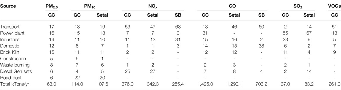
TABLE 3. Sector-wise source contributions (%) to particulate matter and various trace gases.
The chemical lifetime for a species, which has photochemical loss, is defined as the inverse of its total loss rate (Seinfeld and Pandis, 2006). More reactive species will have shorter lifetimes. Particles do not have fast chemical loss like gases but they settle down to various surfaces. Coarse (bigger) particles (such as PM10 and bigger) have shorter lifetime, while the finer (smaller) ones (PM2.5) have longer lifetime (Textor et al., 2006; Croft et al., 2014; Kristiansen et al., 2016). Many species such as SO2 and O3 also have significant loss due to dry deposition. Furthermore, loss rates are higher leading to shorter lifetimes in a polluted atmosphere compared to cleaner regions. Also, chemical lifetimes are shorter in summer than in winter for species having photochemical losses. Williams et al. (2012) have estimated aerosol lifetime as a function of particle size and as a function of altitude using data gathered during Indian Ocean Experiment. They found a lifetime of approximately 1.5 days for aerosols in the boundary layer for particle sizes between 0.08 and 0.1 µm. Larger size particles known as super micron size particles (1.1–10 µm) have shorter residence time. Grythe et al. (2017) found a lifetime of particles greater than 1 µm radius to be less than a day.
O3 has a short lifetime, typically hours, in polluted urban regions where concentrations of its precursors are high (Stevenson et al., 2006; Conley et al., 2012; Young et al., 2013; Monks et al., 2015). Based on the estimated values of hydroxyl radical (OH) over the northern Indian Ocean, which were several times higher than the global average OH concentration of approximately 1 × 10⁶ molecules cm−3, Lawrence and Lelieveld (2010) found lifetime of CO of only ∼15 days near the surface, and a NOx lifetime of less than a day.
The atmospheric lifetime of NOx depends on various processes occurring in the atmosphere including the photolysis of NO2 and the hydroxyl-mediated oxidation of NO2; thus, its lifetime depends on the concentration of other constituents (Levy et al., 1999; Shah et al., 2020). Liu et al. (2016) estimated the NOx lifetime using OMI satellite data and ECMWF wind fields over polluted cities and power plants in polluted background and have found it to be 3.8 ± 1.0 h. The lifetime of SO2 is approximately 1.8 days within the boundary layer depending upon the meteorological conditions and the removal by OH-induced gas-phase conversion into gaseous sulphuric acid (Inomata et al., 2006; Lee et al., 2008).
Figure 3 shows a pictorial representation of COVID-19 effect on anthropogenic air pollution represented by tropospheric column NO2 (Tropo col NO2) changes during COVID-19 months (2020) over the Indian region w.r.t. similar period in the previous year (2019). Most of the boundary layer NO2 can be specifically attributed to its anthropogenic sources, which were the most impacted as a result of lockdown. The effect is clearly visible in much reduced tropospheric column NO2 concentrations during COVID-19 months.
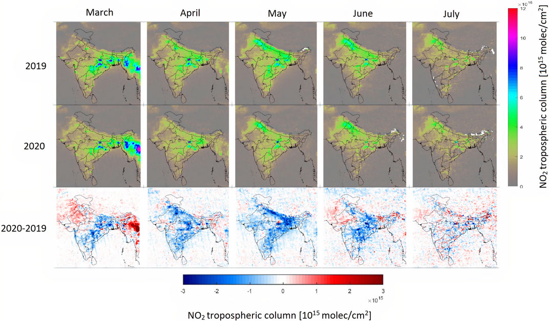
FIGURE 3. Satellite observations of tropospheric column NO2 over the Indian region during the months corresponding to COVID-19 lockdown and unlock phases (March, April, May, June, July) during 2020 (B) and comparison to 2019 (A). (C) shows the monthly difference between 2020 and 2019.
Figure 4 shows monthly average columnar concentration of tropospheric col NO2 over a latitude longitude range of 28.465°N–28.715°N and 77.065°E–77.315°E that covers the NCR around New Delhi. The vertical bars are ±1 sigma standard deviations. A clear decrease of tropospheric column NO2 amount can be seen in the months of April (−45%), May (−42%), and June (−26%). March 2020 does not show a clear decrease because the lockdown was implemented only in the last week of March (Table 1). The decrease in NO2 ceases to be significant in July (−6%) as lockdown measures were restricted to few containment zones (Table 1).
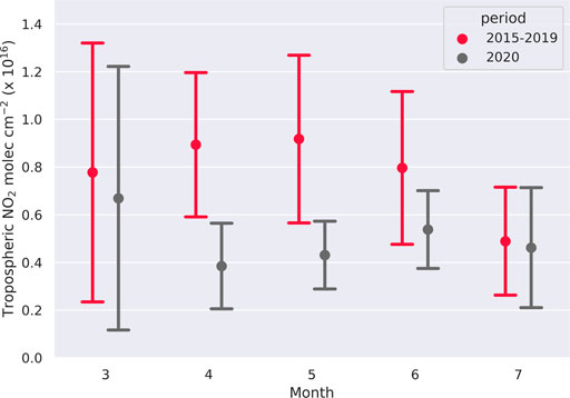
FIGURE 4. OMI retrievals of tropospheric NO2 column over Delhi during months corresponding to COVID-19 lockdown and unlock phases during 2020 and comparison with previous years.
Figure 5 shows monthly average of aerosol optical depth (AOD) over New Delhi. Despite a large year to year and monthly variability, a significant decrease in AOD is observed. Usually an increase in AOD values is observed over Delhi from March to June (Pandithurai et al., 2008) but in 2020, AOD values were low during the lockdown period starting from April to June compared to the same month in previous years. We believe this was because of reduced anthropogenic emissions during the lockdown. A major source of aerosols in Delhi during summer has been found to be fugitive dust particles from roads, and the construction sector accentuated by windblown dust. A receptor-based modeling approach by ARAI and TERI estimated influence of nearly 42% to PM10 and 34% to PM2.5 from this sector for the summer months (ARAI and TERI, 2018). The road transport and the construction works were severely limited during the lockdown period, due to both Government mandate and exodus of migrant workers from Delhi. As a result, the natural increase in AOD was balanced by a decrease from the anthropogenic sector, cumulating into a scenario where AOD remained peculiarly flat during the summer months with lower values during 2020 year compared to previous years (2015–2019) and a decrease in monthly values until June is observed. A recent study revealed that AOD decrease over India during lockdown was of the order of 45%, while the AOD anomaly over Delhi NCR was −24.6% during the 2nd half of April and −44.2% during the first half of May (Ranjan et al., 2020). Furthermore, we observe an enhancement of AOD during March (10.4%) but reductions of 25.3 and 22.5% in April and May respectively when calculating the anomaly against 2015–2019. In June, the AOD values were only 7% lower than the 5 year mean and in July, the AOD values for 2020 were 2.4% higher than 5 year mean. The difference between our estimates and Ranjan et al.’s (2020) estimates is because of the fact that Ranjan et al. have used average from 2000 to 2019 whereas we have used average of 2015–2019 for the comparison (Figure 5B). Another reason could be the resolution of the data used; we have used 0.5 × 0.5 degree area while Ranjan et al. have used very high spatial resolution (1 km) data.
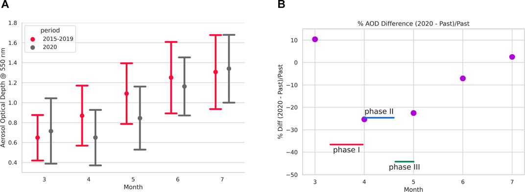
FIGURE 5. (A) VIIRS observations of AOD over Delhi during months corresponding to COVID-19 lockdown and unlock phases during 2020 and comparison with the average of 2015–2019. (B) Percentage changes in AOD; the points show monthly % changes from the present study while the lines show data from Ranjan et al. (2020), with x-span of the line representing the period for which the change is calculated.
The above explanations for AOD and NO2 represent an integrated atmospheric change as a result of COVID-19 lockdown. However, most of the emission changes occur close to the surface. Therefore, we present a detailed analysis of surface observations.
To understand the changes in atmospheric concentrations of trace gases and particulate matter as a result of changed emission scenarios, the daily variation of these parameters during March–July, 2020 is compared with the average of 2015–2019 of the same period and for the same parameters. An example plot for Anand Vihar is shown in Figure 6. It is observed that the two datasets start to diverge around day of year (DOY) -85, representing 25 March, the day of initiation of nationwide lockdown (Table 1). The divergence around this period is maximum for NO2 followed by PM10 and PM2.5. The divergence is also significant in O3. This indicates that the sources impacted by lockdown play a crucial role in the budgets of NO2 and PM (2.5 and 10). The patterns for PM and NO2 are more or less similar for different stations but this does not hold so for O3. This is on expected lines as the major sources of PM e.g., transport sector and road dust account for 30–40% of PM10 over Delhi. Similarly, transport sector makes a major contribution in the anthropogenic NO2 sources. As a result, the departure in NO2 is drastic both in satellite-based columnar data and at surface level (Figures 4, 6). However, not much change is observed for CO, as major sources of CO are related to combustion i.e., biofuels and biomass burning which were not directly affected by lockdown processes. However, O3 presents a different picture as its concentration is a complex interplay of atmospheric transport processes, changes in primary emissions, meteorology and photochemistry in addition to chemical and depositional losses. These changes in surface level pollutants are further discussed below.
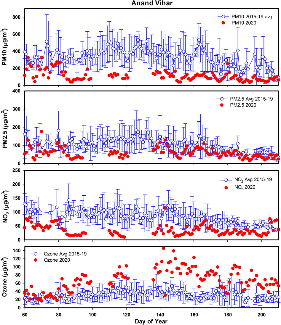
FIGURE 6. Particulate matter and trace gases variations over a representative study location (Anand Vihar), Delhi during months corresponding to COVID-19 lockdown and unlock phases during 2020 and comparison with the average variation during 2015–2019.
High amounts of atmospheric aerosols negatively affect health and air quality, and hence constitute criteria pollutant for the measure of air quality. Indian cities in general suffer from poor air quality mostly due to aerosols (SOGA, 2020). India’s capital city, Delhi, is particularly badly affected by air pollution. In a particularly grave event, PM2.5 concentrations (peak 24 h average 650 µg m−3) exceeded the Indian air quality standards by 11 times and the World Health Organisation (WHO) guidelines by 25 times in early November 2017. Beig et al. (2019) studied this event and found that combined effect of a dust storm in the middle-east, agricultural waste burning in upwind states, and stagnation of local air pollution led to this event. The mortality rate due to pollution in Delhi is estimated to be very high and the city is projected to be among the top 5 cities in the world to have high fatality rates (Apte et al., 2015; Lelieveld et al., 2015). Air pollution caused between 10000 and 30000 premature deaths in Delhi in 2015 (Bithal, 2018). While air pollution is particularly bad in winter over Delhi, the PM2.5 levels are often higher than the WHO limit of 25 µg m−3 and the Indian Air Quality Standard of 60 µg m−3 for most part of year except during the rainy months of July and August (Bali et al., 2019; Hama et al., 2020). Main sources of PM2.5 particles are anthropogenic emissions except when there is a dust storm like event. In a past study, chemical make-up of PM10 aerosol over Delhi was found to be 20% organic, 6% combustion, 31% secondary inorganic, and 43% soil particles during the spring season. While for the most part of India, the residential sector is a major emitter of PM2.5 particles, over Delhi it is the transport sector with nearly 64% contribution (Conibear et al., 2018; Reddington et al., 2019). Beig et al. (2019) attributed 65% of observed PM2.5 concentration to dust and smoke transport from upwind regions for a high pollution event during November 2017. However, this fractionation may not be applicable for all seasons and local emissions may have far more dominating influence on the total concentration. This is because overall wind direction and boundary layer characteristics are different in summer and winter as one can see from the FLEXPART output (Figure 7), as well as the meteorological plots shown in Figure 2. While winter time air pollution over Delhi is studied more frequently because of very high aerosol concentration making them visible and perceptible as a health threat in public mind, concentrations in summer, even though lower than the winter months, are still high enough to pose serious health hazards when exposed for a long time but they are less frequently studied. A campaign-based study during January–March, 2018 over multiple sites in Delhi region using three aerosol mass spectrometers (AMS) for non-refractory fraction, two aethalometers, and one single particle soot photometer concluded that local pollution was dominating over regional pollution during this period (Lalchandani et al., 2021). This was based on the observation of similar chemical composition both within Delhi-NCR and downwind region with mean PM2.5 reaching 153.8 ± 109.4 μg m−3 with major contribution from organics (43–47%) followed by chloride (11–17%), ammonium (9–13%), sulfate (8–13%), nitrate (9–11%), and (5–16%) black carbon. However, significant fraction of highly oxidized, low volatile organic aerosols to the oxygenated organic aerosol (OOA) fraction indicated influence of regional transport, which was attributed to the north-west direction of the study sites. A detailed chemical characterization of PM2.5 over Delhi for heavy and trace elements using the Energy Dispersive X-ray Fluorescence technique during post-monsoon of 2019 concluded large influence from agriculture-residue burning emissions in north-west Indo-Gangetic Plains (IGP) (Bangar et al., 2021). In contrast to winter pattern, during warm season, Jain et al. (2020) observed higher amount of secondary sulphate over secondary nitrate indicating higher contribution from point sources. A higher contribution of secondary organic carbon during pre-monsoon compared to post-monsoon was found over Delhi during a study employing stable carbon isotope analysis (Singh et al., 2021). The study confirmed the dominance of C3 plant-derived aerosols over Delhi, which could be sourced from agriculture residue burning transported from outside the city. Air mass trajectory cluster analysis using HYSPLIT over Delhi during January 2013–June 2014 indicates that the air mass approaches from 4 sides [north-western IGP, Pakistan (10%); north-western IGP, north-west Asia (45%); eastern IGP (38%); Pakistan and Arabian Sea (6%)] (Sharma et al., 2016). The authors concluded that PM10 over Delhi is dominated by soil dust (22.7%) followed by secondary aerosols (20.5%), vehicle emissions (17.0%), fossil fuel burning (15.5%), biomass burning (12.2%), industrial emissions (7.3%), and sea salts (4.8%). The lockdown provided a unique opportunity to study causes of air pollution and evaluate sectoral contributions during the summer months.
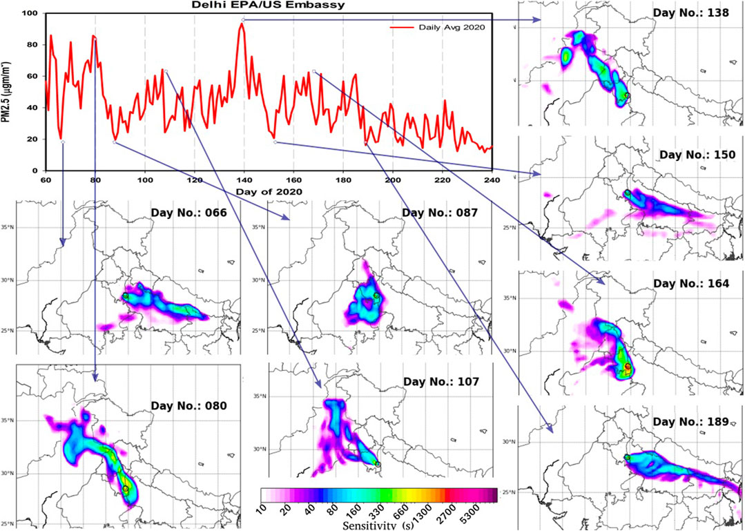
FIGURE 7. FLEXPART-based source region estimations for Delhi during months corresponding to COVID-19 lockdown and unlock phases during 2020 and comparison with previous years. The sensitivity (s) is given in seconds.
Figure 7 shows the source-receptor matrix calculated using FLEXPART for select days when PM2.5 concentrations were observed high or low. The air masses were from the north-west direction during initial phases of lockdown (March), but during later phases after the onset of monsoon over Delhi in June, the air masses became easterly over Delhi, bringing in pollutants from the eastern IGP. Interestingly, in Figure 7, higher peaks in PM2.5 coincide with north-westerly air-masses sourced to industrial regions in Haryana and Punjab of India all the way back to Lahore in Pakistan and further back to the north-west. Lalchandani et al. (2021) have shown through high-precision AMS measurements that air mass transport from north-west air over different sites in Delhi is associated with conspicuous amount of highly volatile and semi-volatile OOA. Higher levels of tropospheric NO2 column values can be seen in the month of May (Figure 3) toward the north-west of Delhi and up to Pakistan in the IGP which suggests heavy pollution due to industrialization in this area. The high patch of NO2 column gets diluted in June as the influence of monsoon winds starts. Lower values of PM2.5 are related to the atmospheric transport either circulating around NCR or coming from the eastern part of IGP, where NO2 columns already evince relatively lower values. Hence, major changes in PM2.5 are likely associated with the transport from the corresponding NO2 column regions.
The PM10 concentration, which is found to be in the range of 80–270 μg m−3 in IGP in the previous years, was reduced to ∼70 μg m−3 during the lockdown. Daily average variations of PM2.5 and surface level NO2 over two nearby study sites in Delhi during the lockdown period are shown in Figures 8A,B against the daily 5 year average of 2015–2019. As mentioned earlier, there is large variability in the 5 year average as well as during the 2020 due to transport of pollutants from the surrounding regions. While there is a general decreasing pattern from May to August because of the change in wind direction, a significant decrease in PM2.5 is seen for the lock-down period despite that. Since lifetime of PM2.5 is only 1–2 days (Table 4), sharp decrease in the levels of PM2.5 was observed from the inception of the lockdown on 25th March (day #85) till at least May end (day #152). The rapid decrease also suggests that anthropogenic emissions are the significant sources of PM2.5 particles over Delhi. Of course, there are two events of high PM2.5, the first from day #90 to day #105 and the second peak around day #140. Similar changes are observed even in NO2 at a nearby location for example at Shadipur as shown in Figure 8B. This shows that these major changes are not local but in a large area covering the NCR and are due to transport from different regions as discussed above using the FLEXPART trajectories. The region in north-west of Delhi seems to contain very large sources of particulate pollution, as whenever the source region is north-west of Delhi, PM2.5 concentrations are high. Aethelometer black carbon measurements over Delhi showed increased local contributions (fossil fuel fraction) with the progress from lockdown to unlock phase, but the fossil fuel contribution specifically dipped during 4–17 May due to intensive crop residue burning in neighboring states (Goel et al., 2021). Gadhavi et al. (2015) who analyzed black carbon concentration over a rural location in South India, also found high concentrations of black carbon particles for the days when the source region extended to north-west of Delhi compared to other days. While looking at the PM2.5 concentration maps available in the literature (Bali et al., 2019; Reddington et al., 2019), one can see whole of IGP region filled with high amount of particles. The temporal variation of PM concentration when looked in connotation with FLEXPART trajectories, east of Delhi region seems to contribute much smaller amount of air pollution compared to when wind is blowing from west.
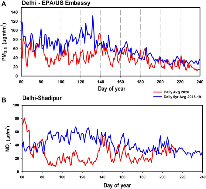
FIGURE 8. (A) PM2.5 variation observed at US Embassy New Delhi during the COVID period from 1 March to 31 July (red curve). It is compared with 5 year period (2015–2019) (blue line). (B) Similar to PM2.5 but for NO2 observed at Shadipur, a location near the US Embassy site.
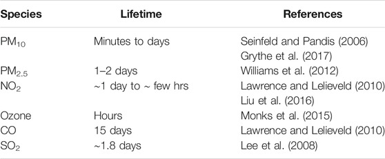
TABLE 4. Lifetimes of particulate matter (PM) and various gaseous species.
Figures 9A,B show monthly average percentage changes in 2020 with respect to the 5 year average of 2015–2019, [(X2020–X2015–2019)/X2015–2019] × 100, in PM10 and PM2.5 respectively. Unfortunately, PM10 data are available only for the 3 stations from the selected locations for this work (Figure 9A). Anand Vihar shows the largest decrease in PM10 as compared with the other two locations, while the other two locations show almost similar changes. Highest decrease of about 73% is observed in April, which was the month of very strict lockdown with almost all transport and industries closed. As the lockdown starts easing during each month, levels of PM10 continue to increase. However, even in July the decrease is significant, smallest approximately 33% for Central Road Research Institute. This could be due to continuation of lockdown for certain activities such as educational institutes, metro services, cinema halls, restricted attendance at offices, limited domestic air travel etc., as listed in Table 1. The major sources of PM10 are transport, industries, brick kiln, and dust from roads and construction activities (Table 4). All these remained closed during the lockdown and slowly and progressively allowed to return to normal. Since the lifetime of PM10 is very short, only a few hours (Table 3), it shows almost an instant effect of the changes. The ratio of decreases between Punjabi Bagh and Central Road Research Institute during different months shows an average value of 1.1, which indicates a uniform impact of lockdown on PM10 from north-west to south-east of urban Delhi (Figure 1). If these ratios are computed with respect to Anand Vihar to the other sites, the value is much higher, revealing that the magnitude of lockdown effect has been larger over this site with respect to PM10. As mentioned in The Study Locations, Anand Vihar is located to the East of River Yamuna, comparatively more congested and impacted by mixed emissions from industries and transport sector. Furthermore, the magnitude of decreases evinces an overwhelming anthropogenic control of PM10 over Delhi.
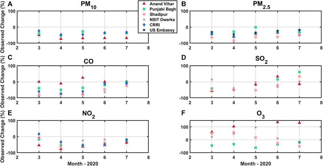
FIGURE 9. Percentage change in monthly mean concentrations at various locations with respect to the average of 2015–2019 for (A) PM10, (B) PM2.5, (C) CO, (D) SO2, (E) NO2, (F) O3.
Changes in the monthly average levels of PM2.5 are shown for all the five locations selected for this work (Figure 9B) and additionally include the EPA data for the US Embassy in Delhi. In general and as for PM10 and also for other species, maximum decrease is observed in April. There is large variability from location to location. Shadipur shows the highest decrease of approximately 83% with respect to the 5 year average followed by Anand Vihar (approximately 61%) and other locations. Again, even in July the levels of PM2.5 have not become normal, with the smallest decrease approximately 18% for the US Embassy. The emission sources of PM2.5 are almost similar to that of PM10 but there is a significant contribution of secondary aerosols to PM2.5. Some studies show almost 50% contribution from secondary aerosols to PM2.5 mass of which nearly 30% is from secondary organic aerosol (Perrino et al., 2011; Rastogi et al., 2014). The formation of secondary aerosols is initiated by various gaseous pollutants such as NOx, SO2 as well as hydrocarbon oxidation. Hence, changes in these precursors also get reflected in the levels of PM2.5. Another source apportionment study estimated daily PM2.5 emissions over Delhi to be 58.7 ton/day, contributed by road dust (38%), vehicles (20%), domestic fuel burning (12%), industrial point sources (11%), concrete batching plant (6%), hotels/restaurants (3%), and municipal solid waste (MSW) burning (3%) (Nagar et al., 2017). Furthermore, the contribution from coal/fly-ash to PM2.5 increased from 4.8% in winter to 26% in summer, while the contribution from secondary inorganic aerosol decreased from 30% in winter to 15% in summer (Nagar et al., 2017). While PM10 decrease was highest for the Anand Vihar site (east Delhi), the PM2.5 decrease was highest over Central Delhi for Shadipur. The ratios of Shadipur to Anand Vihar are 1.6, 1.4, 1.5, 1.7, and 1.6, respectively, for March–July months, with an average of 1.5. This near constant ratio evinces a 50% higher impact to PM2.5 in Central Delhi compared to Eastern Delhi due to lockdown. Possibly, the chances of SOA formation locally can be accentuated by local emissions of precursor gases such as SO2, NO2 and hydrocarbons at Shadipur from industry, transport, and tourism sectors, as new construction activities as well as road dust are very limited over this region. Chemical characterization studies during summer over Delhi have found a higher contribution of SO42-, NO3−, and NH4+ to PM2.5 compared to PM10 (ARAI and TERI, 2018). Source apportionment studies point to potential chloride sources northwest of the Indian Institute of Technology (IIT) Delhi, such as industries of salt and metal processing and thermal power plants to fine PM (Jaiprakash et al., 2017).
Both these species are considered primary pollutants. SO2 contributes to respiratory symptoms. High levels of CO can reduce the amount of oxygen that can be transported in the bloodstream to critical organs such as the heart and the brain resulting in dizziness, confusion, unconsciousness, and even death. Both these species are not very reactive. SO2 is formed during the burning of sulphur containing fuels, such as coal and oil, while CO is formed during the incomplete combustions e.g., fuels such as petrol, coal, or wood. In an urban environment, major sources of CO are transport, domestic cooking, brick kiln, industries, and power plants; while those of SO2 are coal burning in power plants and industries, transport sector, and diesel-generating sets (Table 3). Lifetime of CO is approximately 15 days in a polluted region, while the main sink of SO2 is deposition and has a lifetime of approximately 2 days (Table 4). Data for these two species are available for all the considered locations except for Central Road Research Institute, where SO2 is not available. However, there seem to be large variations.
Figure 9C shows the observed monthly CO changes during 2020 with respect to the 5 year average of 2015–2019. CO shows large decrease in March for Punjabi Bagh, Shadipur, Central Road Research Institute, and NSIT-Dwarka. However, the change is negligible over Anand Vihar in East Delhi. While the decrease continues over Punjabi Bagh and Central Road Research Institute in April, over NSIT-Dwarka there is a negligible increase. The May values show a decrease in Punjabi Bagh, Shadipur, and Central Road Research Institute, while an increase is observed over Anand Vihar and NSIT-Dwarka. The maximum decrease in CO is observed for Central Road Research Institute (approximately 57, 71, 63% in March, April, and May) followed by Punjabi Bagh. Although biogenic emissions constitute a major source of CO, large changes in CO similar to other anthropogenic markers e.g., SO2 indicate overwhelming anthropogenic components in Delhi. In a comprehensive study of air quality in 15 major cities of India using remotely sensed data, surface concentration measurements of CPCB, and Air Quality Zonal Modelling, more than 40% decrease was observed for CO in north Indian cities but for Delhi, an increase of 36% was observed (Rahaman et al., 2021). The study used data covering 43 days before and after lockdown; however, MEERA-2 observations by the same study showed a negligible decrease of 2.52%. The data for Rahaman et al. (2021) are taken from the ITO site at Delhi, which is approximately 7 km from Anand Vihar site, which shows a negligible decrease in CO unlike other sites in our study. On an average, CO decreases by over 50% during March-May, but there is large variability between individual sites e.g., negligible decrease in Anand Vihar to over 90% decrease in NSIT-Dwarka. Based on the data from the 134 observation sites of CPCB, Singh et al. (2020) concluded a decrease of CO over most parts of India. However, for the north-west region, the interquartile range for CO varied from +10% to −40% (Singh et al., 2020).
Large changes in SO2 are observed in the lockdown months of March–May in the order of 35–50% in line with NO2 and PM (Figure 9D). As the major sources of SO2 are large point sources such as power plants, under influence of a given air mass, they are likely to have a similar impact over a larger region. This is evinced by very close values of percent changes during the lockdown months. However, unlike other sites, NSIT-Dwarka did not show a decrease in SO2 during March 2020 (Figure 9D). A closer look at the site data revealed that the overall SO2 levels had been higher in the first quarter of 2020 compared to similar periods in other years. This can be attributed to increasing construction activities in this western edge of urban Delhi including sewage treatment plants. Painting activities at construction sites are also a source of SO2. A good marker of SO2 source types is the SO2 to NO2 ratios. Renuka et al. (2020) have used it to show seasonal variation of sources at a rural site in South India. High SO2 to NO2 ratio indicates predominant impact of point sources such as power plants, while lower values indicate vehicular emissions that are rich in NOx compared to SO2 (Mallik et al., 2015). An increase in this ratio during the initial lockdown phases indicates that the impact of vehicular emissions decreased (reduced denominator in the form of NO2) in comparison with point sources. The increase is particularly very clear over Anand Vihar (figure not shown). The impact of air mass change is also very evident in these ratios e.g., the values were higher over NSIT-Dwarka before onset of pre-monsoon winds indicating larger influence of point sources, while there is a sudden decrease in this ratio since mid of March. After this, as an effect of lockdown, the ratio starts to increase like other sites. Rahaman et al. (2021) have observed approximately 25% decrease in SO2 based on ITO CPCB data while an increase of 23% was observed in a nearby site (Ghaziabad, 30 km east of ITO). Satellite observations over Delhi also showed approximately 40% decrease in the Rahman et al. study. In Singh et al. (2020) study, the variation of SO2 is similar to CO with interquartile range for north-west India between +8% and −38%. Various estimates for SO2 are calculated for Delhi e.g., 9% decrease (Chhikara and Kumar, 2020), 19% decrease (Kumari and Toshniwal, 2020), 23% decrease (Singh et al., 2020), the differences may be attributed to the different periods of estimations, but overall all studies show a decrease.
Oxides of nitrogen such as NO and NO2, together called NOx, are important pollutants emitted from combustion at high temperature. While emissions of NOx are mostly in the form of NO, it is later converted into NO2 by the reaction of NO with O3, HO2, RO2, and other oxidants. During daytime conditions of sufficient O3 and radiation, NO and NO2 are in a fast photochemical equilibrium, or “photo-stationary state.” The photolysis of NO2 during the day is a direct source of tropospheric O3. The NOx concentration determines both the HOx and O3 cycles. At very high concentrations, NO2 can be titrated by OH, eventually leading to HNO3 formation. At very low concentrations, HO2 loss through self-reactions and cross reactions with RO2 lead to net HOx loss. But as NOx increases, the HO2-NO reaction becomes competitive and HO2 is recycled into OH increasing the chain length. Despite a short lifetime, NOx can also be transported from one place to another either in its original gaseous state or in the form of nitrates, PAN etc., and nighttime chemistry becomes important (Levy et al., 1999). In high NOx regimes like urban regions, including Delhi, the production of O3 is generally limited by volatile organic compounds (VOCs). Both NO and NO2 are measured at several locations in Delhi but we discuss results of NO2, here as it is observed at all the locations selected and column NO2 is also measured by satellites. The change in the monthly average levels of NO2 during 2020 compared to the average of 2015–2019 is shown in Figure 9E. While average surface NO2 levels decreased by only 43% for the study sites over Delhi, the average decrease was 57, 50, 40, and 26%, respectively, for April, May, June, and July. On a different perspective, tropospheric NO2 decreased by 57, 53, 32, and −6% for April, May, June, and July i.e., for the same months. The numbers are self-explanatory as April was a complete lockdown and May was a partial lockdown, while in March (average decrease of 14% only), lockdown was implemented in the last week only. The April NO2 levels came down from 30 µg m−3 in the previous years (2015–2019 average) to approximately 11 µg m−3 in the lockdown. Because the major influence on NO2 concentrations is from anthropogenic emissions, the impact of lockdown is nicely traced in surface NO2 measurements. The lowest levels of NO2 among the study sites are observed for NSIT-Dwarka, while the highest levels are observed for Anand Vihar in the east of Delhi. This is because NSIT-Dwarka is a more planned area with open spaces and airport, while Anand Vihar is congested with multiple emission sources. Furthermore, it is to be noted that Anand Vihar has a major inter-state bus terminal and the bus service as well as local travel is still not to full scale. Punjabi Bagh and Shadipur show almost similar patterns from 2015 to 2020, including the sudden decrease during the lockdown. The maximum change by approximately 76% is observed in April at Anand Vihar. As the lockdown is relaxed gradually, the 2020 levels start coming toward the normal. The decrease at Anand Vihar became approximately 38% in July. Levels of NO2 at other locations also have not come to normal levels. An early study of lockdown effect on NO2 for different states of India using Aura/OMI data revealed that among the other states of India, the maximum decrease was observed over Delhi (62% over 2019 values and 54% over 2015–2019 average values) with higher decrease in phase I (25 March–14 April, 2020) compared to phase 2 (15 April–3 May, 2020) (Pathakoti et al., 2020). Similar decreases over Delhi were concluded by various studies: 63.9% (Bedi et al., 2020), 42.27% (Chhikara and Kumar, 2020), 60% (Kumari and Toshniwal, 2020), 56% (Singh et al., 2020); the differences being the varied periods for averaging as well as varying reference periods. Even in our study, in contrast to SO2, the variability of NO2 among different stations exhibited an overall decrease from March to April to May to June. This indicates that as lockdown measures strengthened from March to April, people settled in their homes leading to minimum vehicular and industrial emissions, decrease in both NO2 levels as well as the variability between different sites in Delhi was evident. The homogeneity between sites strengthened until May as people settled into similar patterns of life with similar patterns of emissions. This continued even in June when values started to increase with relaxations in activities, but the pattern remained similar leading to lower variability in terms of decrease in different sites in Delhi (Figure 9E; Table 1).
The daytime chemical production and loss of surface O3 in the troposphere is controlled by competing reactions involving many of its precursors such as NO2, NO, CO and hydrocarbons in the presence of sunlight (Seinfeld and Pandis, 2006). It is produced by the reaction of atomic oxygen with molecular oxygen as in the stratosphere. However, this atomic oxygen does not come from the dissociation of molecular oxygen as in the stratosphere but from the dissociation of NO2 as shown in the following simple reactions scheme.
OH is produced from the reaction of water with O(1D), which in turn is produced from the photolysis of O3 at wavelengths <320 nm.
In the absence of competing reactions, the net effect of reactions R4, R5, and R9 is zero. The reaction of OH initiates the breakdown of CO and VOCs, resulting in the formation of ROx (e.g., R1). The simplest is HO2, formed from the oxidation of CO to CO2. While radical-radical self and cross reactions are dominant at low NO, with increasing NOx, NO gradually outcompetes the peroxide-forming reactions, leading to rapid recycling between OH and HO2. At very high concentrations, there is net loss in the form of HNO3, while at very low concentrations of NOx, there is HOx loss in the form of peroxides. Depending on VOC to NOx ratio, the oxidation capacity increases at intermediate NOx levels. Mertens et al. (2021) employed a combination of regional chemistry climate model (CCM-COSMO) and global chemistry climate model (CCM_EMAC) with a general circulation base model (ECHAM5) to make a sector-wise attribution of O3 changes resulting out of emission reductions during the lockdown over Europe. Interestingly, the authors found that despite reduced O3 production due to reduced anthropogenic emissions, the O3 production efficiency (OPE) i.e., net O3 production per molecule of NOx increased. It was also observed that the ratio of H2O2 (HO2 sink) to HNO3 (OH sink) production rates exhibited an enhancement during the lockdown period indicating a shift from NOx-saturated to NOx-limited regime. Despite increased OPE, there was a net O3 reduction as anthropogenic emission reduction overcompensated the enhanced OPE and natural emissions. Furthermore, as O3 has a fairly long lifetime, the impact of atmospheric transport can compensate for immediate chemical changes in a region. In another study, sensitivity of global tropospheric O3 burden to anthropogenic NOx reductions (COVID-2020 emission anomaly over 2010–2019) was studied employing the state-of-the-art multi-constituent satellite data assimilation system, which was used to ingest multiple satellite observations to simultaneously optimize concentrations and emissions of trace species and simulating their chemical interaction (Miyazaki et al., 2021). Strong O3 response to NOx reductions in highly polluted areas attributed to NOx titrations and enhanced oxidation capacity led to local O3 enhancements. The role of atmospheric transport was revealed in Miyazaki et al. study such that O3 reductions in Central Eastern Eurasia were attributed to emission reductions over North America. In this study, global reductions were also estimated for peroxyacetyl nitrate (NOx reservoir) and OH. Using generalized additive models fed by reanalysis meteorological data, Ordóñez et al. (2020) showed that while NO2 concentration variations in Europe were attributed to reduced emissions, O3 concentration changes were mostly explained by meteorology. Over Delhi, O3 reduction upto 13% was observed by Datta et al. (2021); the authors use statistical analysis to show that O3 concentration variations were not explained by lockdown effects unlike PM variations, which were largely contributed by lockdown-induced emission changes.
Community Multi-Scale Air Quality (CMAQ) model estimations revealed that during lockdown, there was a 15% decrease in maximum daily 8 h average (MDA8) O3 (Zhang et al., 2021). However, in some VOC-limited urban regions, O3 enhancement was observed mainly due to higher reduction of NOx compared to VOCs. If both VOCs and NOx are low for example in the pristine regions, production of O3 is very low. If both are high for example in a polluted urban region, high levels of O3 can be produced (Seinfeld and Pandis, 2006). In the intermediate regime, O3 production or loss depends upon the levels of NOx and hydrocarbons. The transition from VOC-limited to NOx-limited regimes can be gauged through various proxies. OPE (i.e., ΔO3/ΔNOz) is a simple measure to infer the O3 formation regimes with values less than 4 indicating VOC limited and greater than 7 indicating NOx limited (Wang et al., 2017). Another popular proxy is the ratio of OH-reactivity of NOx to OH-reactivity of VOC (Sinha et al., 2012). If this ratio exceeds 0.2 (±0.1), the O3 production regime is VOC limited, whereas if it is below 0.01, the O3 production regime is considered NOx limited. The intermediate range, 0.01 < 2 < 0.2, indicates that the peak O3 production depends strongly on both NOx and VOC levels. Furthermore, as the production of HCHO is proportional to reactions of reactive organics with OH, the HCHO/NOy ratio can also be used to segregate the two regimes with 0.28 marking the transition from VOC limited to NOx limited (Sillman, 1995).
In the VOC-limited regime, decreasing VOC emissions reduces the chemical production of organic radicals (RO2), leading to decreased cycling with NOx thus reducing O3 (Wang et al., 2021). In the NOx-limited regime, decreasing NOx emission reduces NO2 photolysis, directly reducing O3. In contrast, in the VOC-limited regime, NOx acts to reduce O3, so decreased NOx emissions promote O3 production (Kleinman, 1994). Furthermore, in the NOx-limited regime (or VOC-saturated), O3 production is proportional to square root of HOx (OH + HO2) production while in the VOC-limited (or NOx-saturated) regime, O3 production is directly proportional to HOx production. A WRF-Chem modelling study revealed that the IGP region (including Delhi) is in a NOx to VOC transition regime (Chutia et al., 2019). A box model study using the NCAR master mechanism found that O3 production in Delhi/NCR is limited by the abundance of VOCs even though NOx is higher (Chen et al., 2021). In such VOCs-limited regimes, a decrease in NOx would lead to enhancement in O3. During the lockdown most of the vehicular emissions came to total halt except emergency vehicles. Various industries were closed as well as many other anthropogenic sources of emissions of these pollutants. However, power generation did not stop but got reduced. Major sources of NOx in Delhi are transport, industries, and diesel generator sets (Table 3). All these three sources were almost closed during the lockdown. Similarly, major sources of VOCs include transportation (∼50%), brick kiln, and power plants (Guttikunda and Calori, 2013). The first two were totally closed during the lockdown. So the lockdown would lead to a much larger reduction in NOx. However, in the absence of VOC measurements over Delhi, it will be difficult to quantify the transition regions from VOC limited to NOx limited.
Surface O3 shows different features at different study sites in Delhi (Figure 9F). The O3 results for the Central Road Research Institute are not used here as there are often breaks in the data. One explanation for this variation is related to the ratio of VOCs to NOx. A clear increase in O3 values is observed over Anand Vihar and NSIT-Dwarka, while the unlock phase brings back the O3 values down. In a normal scenario, spring peak in O3 is observed over Delhi as a result of biomass burning in the adjoining areas. Over Shadipur and NSIT-Dwarka, the levels had been similar before lockdown and all were showing a gradual increase from February to March. However, over Anand Vihar and Punjabi Bagh, the increase was not gradual but there had been a decrease in the 1st week of March followed by an increase just before lockdown. However, since the onset of lockdown, O3 over Anand Vihar continued to increase and daily average remained over 60 μg m−3 until air masses changed in late June when O3 levels started coming down. NSIT-Dwarka, located on the western part of Delhi, also showed concurrent features like Anand Vihar (east Delhi) increasing till Phase 3. However, in Phase 3, as relaxations start in transport services, the plummet in O3 levels coincided exactly with an increase in NO2. This shows that during lockdown, as anthropogenic emissions decreased, O3 over Delhi which is normally in a VOC-limited regime is now controlled by titration effects with NOx. The feature is specifically visible over NSIT-Dwarka, where overall NOx levels are lower among the studied sites and decreased further during lockdown (Figure 10). The O3-NOx relationships show different patterns between pre-lockdown, lockdown, and unlock periods at different sites. For instance, over Punjabi Bagh and Anand Vihar, lockdown and unlock data are indiscernible while over Shadipur and NSIT Dwarka, there is a distinct reduction in O3 levels between lockdown and unlock periods. It must be mentioned here that for these O3-NOx relationships, we have not considered the variation of VOCs. However, since these are natural atmospheric data, VOCs in Figure 10, although not shown (due to nonavailability of data), would also be different for each individual point. As mentioned before from the Zhang et al. (2021) analysis, NOx reductions are likely to be much larger than VOC reductions. This is because the major sources of NOx are few and were severely impacted by the lockdown e.g., vehicular emissions but VOC sources are much more varied and all were not impacted by lockdown e.g., residential emissions.
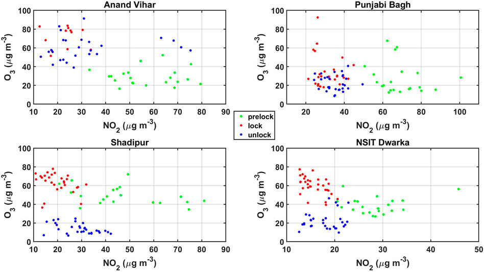
FIGURE 10. O3-NO2 relationships for different lockdown phases and for different study sites.
India started taking precaution in the initial phase of the spread of the corona virus by imposing strict lockdown from 25th March, 2020 itself. This led to closing down of all the industrial activities, all kinds of travel, educational institutes and people were asked to remain in their houses. We studied the impact of these closed anthropogenic sources of emissions during the lockdown from 25th March to almost May end and later unlocking of these till the end of July 2020 at 5 selected locations covering Delhi using in-situ measurements and satellite-based measurements of important pollutants. Daily and monthly average values of these pollutants for 2020 were compared with the 5-year average values from 2015 to 2019. Satellite-based measurements of monthly average AOD and tropospheric column of NO2 for the entire Delhi showed changes from the 5 year average and are listed in Table 5. Comparing the average decrease of different species, it was observed that the species most affected by the lockdown as observed for April data are PM (includes both fine and coarse modes), NO2 (includes both surface level and tropospheric column), and CO. In terms of percentage changes, the different species (except AOD and O3) were clumped together in April when lockdown was in full force. Overall O3 showed an increase over Delhi while AOD showed a much lower decrease compared to PM. The large decrease for CO during lockdown indicates predominant contributions of anthropogenic sources in Delhi for this species. Similar decreases in both surface and columnar NO2 during March-June indicate dominant contribution of surface sources to NO2 columns over Delhi. While tropospheric col NO2 concentrations during COVID-19 months decreased by −56.9%, −53%, and −32.4% in April, May, and June, the AOD values decreased only by −25.3% in April, 2020 with respect to the 5 years average. These slow changes in AOD continued with −22.5% and −7.1% in May and June respectively. By July 2020, the AOD values have almost become normal. It is to be noted that AOD showed much lower decrease than tropospheric column NO2. A similar difference is also observed by Pope et al. (2018). This could be due to the fact that loss of aerosols through deposition occurs near the Earth’s surface. The smaller aerosols in the boundary layer as well as in the free troposphere coagulate to form bigger particles, which also contribute to AOD. The lifetimes of aerosols near the surface are very short as mentioned in Table 4 but much longer in the free troposphere. So when emission of aerosols reduces at the surface, column values (AOD) do not change that much. However, NO2 is photochemically dissociated to form NO, which is highly reactive and reacts with various gases forming nitrates as well as reforming NO2. This happens even more at the higher heights due to intense solar radiation. Hence, when the supply from the emission sources at the surface reduces, column NO2 also reduces.
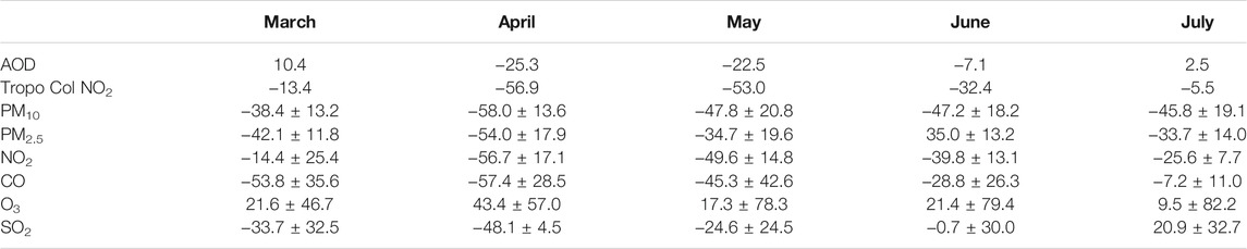
TABLE 5. Average combined percentage change for all the stations considered here as representative for changes in Delhi in monthly mean concentrations of various species during COVID-19 months with respect to average of 2015–19.
The in-situ measurements of surface level PM10 and PM2.5 also showed maximum decrease of −58% and −54% respectively for April, 2020. However, there was a significant decrease in March itself for both the species by −38.4% and −42.1% respectively for PM10 and PM2.5. This was due to 8 days of lockdown in March coupled to seasonal change in wind direction resulting in different source regions. A decrease of −45.8% and −33.7% was observed in July also for both these species even during the second unlock phase. Also, PM10 showed slightly more decrease than PM2.5 in the same period. This could be because of the lifetime of PM10 being shorter than PM2.5 (Table 4). Decrease in NO2 was almost similar to that of PM10 and PM2.5. Major sources of aerosols and NO2 are transport and industries (Table 3), which were totally closed during the first two phases of the lockdown. Although biogenic emissions constitute a major source of CO, large changes in CO similar to other anthropogenic markers e.g., SO2 indicate overwhelming anthropogenic components in Delhi. It is to be noted that the lifetime of CO is much higher than that of SO2 and other species. Singh et al. (2020) have analyzed data for the Indian region and have shown an average decrease in PM10, PM2.5, NO2, and CO by about −58%, −45%, −50%, and −38% respectively.
O3, as discussed in Section 4.6, has complex chemistry depending not only on the levels of its precursors but also on the balance of NOx and hydrocarbons. Model estimates for Delhi show that it is hydrocarbon controlled (Chen et al., 2021). We observed mixed signals (increase as well as decrease) in the levels of O3 at different locations. This could be possible due to different combinations of NOx and hydrocarbons, as these locations have different emission sources, some are heavily transport (NOx) impacted, while others have higher hydrocarbon emissions. During lockdown, as anthropogenic emissions decreased, O3 over Delhi which is normally in a VOC-limited regime is now controlled by NOx. The feature is specifically visible over NSIT-Dwarka, where overall NOx levels were lower among the studied sites and decreased further during lockdown. A clear increase in O3 values was observed over Anand Vihar and NSIT-Dwarka, while the unlock phase evinced a fall in the O3 values. Singh et al. (2020) have found mixed variations in O3 due to lockdown in different parts of India. Similar studies from China and Europe found slight increases in O3 levels during the lockdown (Shi and Brasseur, 2020; Xu et al., 2020; Sicard et al., 2020).
Overall, the effect on the levels of pollutants was mainly due to the reduced vehicular emissions and atmospheric transport from the surrounding regions as well as due to power generation and other point sources. The higher peaks in PM2.5 coincide with north-westerly air-masses sourced to industrial regions in Haryana and Punjab of India all the way back to Lahore in Pakistan and further back to the north-west. Simultaneously, higher levels of tropospheric NO2 column values were observed in the month of May toward the north-west of Delhi and up to Pakistan in the IGP which suggests heavy pollution due to industrialization in this area acting as a source for Delhi. The ratio of decreased PM10 between Punjabi Bagh and Central Road Research Institute during different months showed an average value of 1.1, which indicates a uniform impact of lockdown on PM10 from north-west to south-east of urban Delhi. However for PM2.5, the ratios of Shadipur to Anand Vihar are 1.6, 1.4, 1.5, 1.7, and 1.6, respectively, for March to July months, with an average of 1.5. This near constant ratio evinces a 50% higher impact on PM2.5 in Central Delhi compared to Eastern Delhi due to lockdown. It is to be noted that the lockdown was all over India. We have seen that Delhi gets affected from the surrounding regions, states, as well as even from the nearby countries such as Pakistan and Afghanistan (Figure 7). Hence, these effects are cumulative. In this context, it is worth mentioning that the control of pollution by the local government through restriction of odd-even vehicular movement (only 4 wheelers and in Delhi city only) did not yield the desired results (Chandra et al., 2018).
Hence, changes in the levels of various pollutants during the lockdown-2020 were variable depending upon the emission sources, lifetimes, and chemistry. These results are very useful for testing and updating the emission inventories as well as for models.
Publicly available datasets were analyzed in this study. This data can be found here: https://app.cpcbccr.com/ccr/#/caaqm-dashboard/caaqm-landing/caaqm-comparison-data.
CM: conceptualization, overall data analysis, review and write-up. HG: FlexPart and AOD data analysis, review and write-up. SL: conceptualization, overall data analysis, review and write-up. RKY: NO2 columnar data analysis, review and editing. RB: data analysis, review and editing. TD: data analysis, review and editing.
The authors declare that the research was conducted in the absence of any commercial or financial relationships that could be construed as a potential conflict of interest.
All claims expressed in this article are solely those of the authors and do not necessarily represent those of their affiliated organizations, or those of the publisher, the editors and the reviewers. Any product that may be evaluated in this article, or claim that may be made by its manufacturer, is not guaranteed or endorsed by the publisher.
We acknowledge that OMI NO2 column data were downloaded from https://disc.gsfc.nasa.gov/. VIIRS AOD data were downloaded from https://ladsweb.modaps.eosdis.nasa.gov/. The reanalysis data of meteorology were downloaded from https://rda.ucar.edu/datasets/ds083.2/. Authors thank science teams and personnel associated with generating these data. The FLEXPART model was downloaded from https://www.flexpart.eu/. Authors thank developers and scientists associated with FLEXPART model development. SL is grateful to the Director PRL, Ahmedabad and to CSIR, New Delhi for their support for his position. TD and RB are grateful to Director CSIR-IMMT, Bhubaneswar for support and ISRO-GBP (ATCTM) for funding. Authors sincerely thank the two reviewers for their constructive comments that has improved the MS to its present form. We also thank the editor for quick and timely processing of the MS.
1https://archive.pib.gov.in/archive2/erelease.aspx (Release IDs: 200168 & 200237)
2https://www.mha.gov.in/notifications/circulars-covid-19
3https://www.mha.gov.in/sites/default/files/MHAorder%20copy_0.pdf
4https://www.populationu.com/in/delhi-population
5http://delhiplanning.nic.in/sites/default/files/2%29%20Demographic%20Profile.pdf
6http://delhiplanning.nic.in/sites/default/files/12%29%20Transport.pdf
7https://transport.delhi.gov.in/sites/default/files/All-PDF/Total%2BVehicles%2BRegistered%2Bupto%2B31.03.2018.pdf
9https://app.cpcbccr.com/ccr/#/caaqm-dashboard/caaqm-landing/caaqm-comparison-data
10https://app.cpcbccr.com/ccr_docs/FINAL-REPORT_AQI_.pdf
11https://giovanni.gsfc.nasa.gov/giovanni/
12https://ladsweb.modaps.eosdis.nasa.gov/
Andrews, M., Areekal, B., Rajesh, K., Krishnan, J., Suryakala, R., Krishnan, B., et al. (2020). First Confirmed Case of COVID-19 Infection in India: A Case Report. Indian J. Med. Res. 151 (5), 490–492. doi:10.4103/ijmr.IJMR_2131_20
Apte, J. S., Marshall, J. D., Cohen, A. J., and Brauer, M. (2015). Addressing Global Mortality from Ambient PM2.5. Environ. Sci. Technol. 49 (13), 8057–8066. doi:10.1021/acs.est.5b01236
ARAI and TERI (2018). Executive SUmmary: Source Apportionment of PM2.5 & PM10 of Delhi NCR for Identification of Major Sources. Report No. ARAI/16-17/DHI-SA-NCR/Exec_Summ. Available at: https://www.teriin.org/sites/default/files/2018-08/Exec-summary.pdf
Bali, K., Dey, S., Ganguly, D., and Smith, K. R. (2019). Space-time Variability of Ambient PM2.5 Diurnal Pattern over India from 18-years (2000-2017) of MERRA-2 Reanalysis Data. Atmos. Chem. Phys. Discuss., 1–23. doi:10.5194/acp-2019-731
Bangar, V., Mishra, A. K., Jangid, M., and Rajput, P. (2021). Elemental Characteristics and Source-Apportionment of PM2.5 during the Post-monsoon Season in Delhi, India. Front. Sustain. Cities 3, 648551. doi:10.3389/frsc.2021.648551
Bedi, J. S., Dhaka, P., Vijay, D., Aulakh, R. S., and Gill, J. P. S. (2020). Assessment of Air Quality Changes in the Four Metropolitan Cities of India during COVID-19 Pandemic Lockdown. Aerosol Air Qual. Res. 20, 2062–2070. doi:10.4209/aaqr.2020.05.0209
Beig, G., Srinivas, R., Parkhi, N. S., Carmichael, G. R., Singh, S., Sahu, S. K., et al. (2019). Anatomy of the winter 2017 Air Quality Emergency in Delhi. Sci. Total Environ. 681, 305–311. doi:10.1016/j.scitotenv.2019.04.347
Bithal, S. (2018). Delhi Loses 80 Lives to Air Pollution Every Day, Says Study: Outdoor Air Pollution Is the Fifth Largest Killer in India, Down to Earth published on, , https://www.downtoearth.org.in/news/delhi-loses-80-lives-to-air-pollution-every-day-says-study-50222 (Accessed 10 Dec 2018).
Chandra, B. P., Sinha, V., Hakkim, H., Kumar, A., Pawar, H., Mishra, A. K., et al. (2018). Odd-even Traffic Rule Implementation during winter 2016 in Delhi Did Not Reduce Traffic Emissions of VOCs, Carbon Dioxide, Methane and Carbon Monoxide. Curr. Sci. 114 (6), 1318–1325. doi:10.18520/cs/v114/i06/1318-1325
Chen, Y., Beig, G., Archer-Nicholls, S., Drysdale, W., Acton, W. J. F., Lowe, D., et al. (2021). Avoiding High Ozone Pollution in Delhi, India. Faraday Discuss. 226, 502–514. doi:10.1039/D0FD00079E
Chhikara, A., and Kumar, N. (2020). COVID-19 Lockdown: Impact on Air Quality of Three Metro Cities in India. ajae 14 (4), 378–393. doi:10.5572/ajae.2020.14.4.378
Chutia, L., Ojha, N., Girach, I. A., Sahu, L. K., Alvarado, L. M. A., Burrows, J. P., et al. (2019). Distribution of Volatile Organic Compounds over Indian Subcontinent during winter: WRF-Chem Simulation versus Observations. Environ. Pollut. 252, 256–269. doi:10.1016/j.envpol.2019.05.097
Conibear, L., Butt, E. W., Knote, C., Arnold, S. R., and Spracklen, D. V. (2018). Residential Energy Use Emissions Dominate Health Impacts from Exposure to Ambient Particulate Matter in India. Nat. Commun. 9, 617. doi:10.1038/s41467-018-02986-7
Conley, S. A., Faloona, I. C., Lenschow, D. H., Campos, T., Heizer, C., Weinheimer, A., et al. (2011). A Complete Dynamical Ozone Budget Measured in the Tropical marine Boundary Layer during PASE. J. Atmos. Chem. 68, 55–70. doi:10.1007/s10874-011-9195-0
Croft, B., Pierce, J. R., and Martin, R. V. (2014). Interpreting Aerosol Lifetimes Using the GEOS-Chem Model and Constraints from Radionuclide Measurements. Atmos. Chem. Phys. 14, 4313–4325. doi:10.5194/acp-14-4313-2014
Datta, A., Rahman, M. H., and Suresh, R. (2021). Did the COVID‐19 Lockdown in Delhi and Kolkata Improve the Ambient Air Quality of the Two Cities? J. Environ. Qual. 50 (2), 485–493. doi:10.1002/jeq2.20192Epub 2021 Jan 25
Dhaka, S. K., Chetna, V. K., Dimri, A. P., Singh, N., et al. (2020). PM2.5 Diminution and Haze Events over Delhi during the COVID-19 Lockdown Period: an Interplay between the Baseline Pollution and Meteorology. Sci. Rep. 10, 13442. doi:10.1038/s41598-020-70179-8
Gadhavi, H. S., Renuka, K., Kiran, V. R., Jayaraman, A., Stohl, A., Klimont, Z., et al. (2015). Evaluation of black carbon emission inventories using a Lagrangian dispersion model a case study over southern India. Atmos. Chem. Phys. 15, 1447–1461. doi:10.5194/acp-15-1447-2015
Goel, V., Hazarika, N., Kumar, M., Singh, V., Thamban, N. M., and Tripathi, S. N. (2021). Variations in Black Carbon Concentration and Sources during COVID-19 Lockdown in Delhi. Chemosphere 270, 129435. doi:10.1016/j.chemosphere.2020.129435
Grythe, H., Kristiansen, N. I., Groot Zwaaftink, C. D., Eckhardt, S., Ström, J., Tunved, P., et al. (2017). A New Aerosol Wet Removal Scheme for the Lagrangian Particle Model FLEXPART V10. Geosci. Model. Dev. 10, 1447–1466. doi:10.5194/gmd-10-1447-2017
Guttikunda, S. K., and Calori, G. (2013). A GIS Based Emissions Inventory at 1 Km × 1 Km Spatial Resolution for Air Pollution Analysis in Delhi, India. Atmos. Environ. 67, 101–111. doi:10.1016/j.atmosenv.2012.10.040
Hama, S. M. L., Kumar, P., Harrison, R. M., Bloss, W. J., Khare, M., Mishra, S., et al. (2020). Four-year Assessment of Ambient Particulate Matter and Trace Gases in the Delhi-NCR Region of India. Sust. Cities Soc. 54, 102003. doi:10.1016/j.scs.2019.102003
Inomata, Y., Iwasaka, Y., Osada, K., Hayashi, M., Mori, I., Kido, M., et al. (2006). Vertical Distributions of Particles and Sulfur Gases (Volatile Sulfur Compounds and SO2) over East Asia: Comparison with Two Aircraft-Borne Measurements under the Asian Continental Outflow in Spring and Winter. Atmos. Environ. 40, 430–444. doi:10.1016/j.atmosenv.2005.09.055
Jain, S., Sharma, S. K., Vijayan, N., and Mandal, T. K. (2020). Seasonal Characteristics of Aerosols (PM2.5 and PM10) and Their Source Apportionment Using PMF: A Four Year Study over Delhi, India. Environ. Pollut. 262, 114337. doi:10.1016/j.envpol.2020.114337
Jain, S., and Sharma, T. (2020). Social and Travel Lockdown Impact Considering Coronavirus Disease (COVID-19) on Air Quality in Megacities of India: Present Benefits, Future Challenges and Way Forward. Aerosol Air Qual. Res. 20 (6), 1222–1236. doi:10.4209/aaqr.2020.04.0171
Jaiprakash, S. A., Habib, G., Raman, R., and Gupta, T. (2017). Chemical characterization of PM1 aerosol in Delhi and source apportionment using positive matrix factorization. Environ. Sci. Pollut. Res. 24, 445–462. doi:10.1007/s11356-016-7708-8
Kleinman, L. I. (1994). Low and High NOxtropospheric Photochemistry. J. Geophys. Res. 99, 16831–16838. doi:10.1029/94jd01028
Kristiansen, N. I., Stohl, A., Olivié, D. J. L., Croft, B., Søvde, O. A., Klein, H., et al. (2016). Evaluation of Observed and Modelled Aerosol Lifetimes Using Radioactive Tracers of Opportunity and an Ensemble of 19 Global Models. Atmos. Chem. Phys. 16, 3525–3561. doi:10.5194/acp-16-3525-2016
Krotkov, N. A., Lamsal, L. N., Marchenko, S. V., Bucsela, E. J., and Swartz, W. H. (2019). OMI/Aura Nitrogen Dioxide (NO2) Total and Tropospheric Column 1-orbit L2 Swath 13x24 Km V003. Greenbelt, MD, USA: Goddard Earth Sciences Data and Information Services Center (GES DISC). Joiner, J. and the OMI core team. doi:10.5067/Aura/OMI/DATA2017
Kumari, P., and Toshniwal, D. (2020). Impact of Lockdown Measures during COVID-19 on Air Quality- A Case Study of India. Int. J. Environ. Health Res. 00 (00), 1–8. doi:10.1080/09603123.2020.1778646
Lalchandani, V., Kumar, V., Tobler, A., M. Thamban, N., Mishra, S., Slowik, J. G., et al. (2021). Real-time Characterization and Source Apportionment of fine Particulate Matter in the Delhi Megacity Area during Late winter. Sci. Total Environ. 770, 145324. doi:10.1016/j.scitotenv.2021.145324
Lamsal, L. N., Krotkov, N. A., Vasilkov, A., Marchenko, S., Qin, W., Yang, E.-S., et al. (2020). OMI/Aura Nitrogen Dioxide Standard Product with Improved Surface and Cloud Treatments. Atmos. Meas. Tech. 14 (1), 455–479. doi:10.5194/amt-2020-200
Lawrence, M. G., and Lelieveld, J. (2010). Atmospheric pollutant outflow from southern Asia: a review. Atmos. Chem. Phys. 10, 11017–11096. doi:10.5194/acp-10-11017-2010
Le, T., Wang, Y., Liu, L., Yang, J., Yung, Y. L., Li, G., et al. (2020). Unexpected Air Pollution with Marked Emission Reductions during the COVID-19 Outbreak in China. Science 369 (6504), 702–706. doi:10.1126/science.abb7431
Lee, C., Richter, A., Lee, H., Kim, Y. J., Burrows, J. P., Lee, Y. G., et al. (2008). Impact of Transport of Sulfur Dioxide from the Asian Continent on the Air Quality over Korea during May 2005. Atmos. Environ. 42, 1461–1475. doi:10.1016/j.atmosenv.2007.11.006
Lelieveld, J., Evans, J. S., Fnais, M., Giannadaki, D., and Pozzer, A. (2015). The contribution of outdoor air pollution sources to premature mortality on a global scale. Nature 525, 367–371. doi:10.1038/nature15371
Levelt, P. F., Van Den Oord, G. H. J., Dobber, M. R., Malkki, A., Visser, H., Vries, J., et al. (2006). The Ozone Monitoring Instrument. IEEE Trans. Geosci. Remote Sensing 44, 1093–1101. doi:10.1109/tgrs.2006.872333
Levy, H., Moxim, W. J., Klonecki, A. A., and Kasibhatla, P. S. (1999). Simulated Tropospheric NOx: Its Evaluation, Global Distribution and Individual Source Contributions. J. Geophys. Res. 104, 26279–26306. doi:10.1029/1999JD900442
Levy, R. C., Mattoo, S., Sawyer, V., and Munchak, L. A. (2020). AERDT_L2_VIIRS_SNPP - VIIRS/SNPP Dark Target Aerosol L2 6-Min Swath 6 Km. accessed on: 2020-09-01. doi:10.5067/VIIRS/AERDT_L2_VIIRS_SNPP.001
Levy, R. C., Munchak, L. A., Mattoo, S., Patadia, F., Remer, L. A., and Holz, R. E. (2015). Towards a Long-Term Global Aerosol Optical Depth Record: Applying a Consistent Aerosol Retrieval Algorithm to MODIS and VIIRS-Observed Reflectance. Atmos. Meas. Tech. 8, 4083–4110. doi:10.5194/amt-8-4083-2015
Liu, F., Beirle, S., Zhang, Q., Dörner, S., He, K., and Wagner, T. (2016). NOx Lifetimes and Emissions of Cities and Power Plants in Polluted Background Estimated by Satellite Observations. Atmos. Chem. Phys. 16, 5283–5298. doi:10.5194/acp-16-5283-2016
Mahato, S., Pal, S., and Ghosh, K. G. (2020). Effect of Lockdown amid COVID-19 Pandemic on Air Quality of the Megacity Delhi, India. Sci. Total Environ. 730, 139086. doi:10.1016/j.scitotenv.2020.139086
Mallik, C., and Lal, S. (2011). Changing Long-Term Trends in Tropospheric Temperature over Two Megacities in the Indo-Gangetic Plain. Curr. Sci. 101 (5), 637–644.
Mallik, C., Venkataramani, S., and Lal, S. (2015). Trace gases over a semi-arid urban site in western India: variability and inter-correlations. J. Atmos. Chem. 72, 143–164. doi:10.1007/s10874-015-9311-7
Mallik, C., Chandra, N., Venkataramani, S., and Lal, S. (2016). Variability of Atmospheric Carbonyl Sulfide at a Semi-arid Urban Site in Western India. Sci. Total Environ. 551-552, 725–737. doi:10.1016/j.scitotenv.2016.02.014
Mertens, M., Jöckel, P., Matthes, S., Nützel, M., Grewe, V., and Sausen, R. (2021). COVID-19 Induced Lower-Tropospheric Ozone Changes. Environ. Res. Lett. 16 (6), 064005. doi:10.1088/1748-9326/abf191
Miyazaki, K., Bowman, K., Sekiya, T., Takigawa, M., Neu, J. L., Sudo, K., et al. (2021). Global Tropospheric Ozone Responses to Reduced NOx Emissions Linked to the COVID-19 Worldwide Lockdowns. Sci. Adv. 7, eabf7460. 09 Jun 2021. doi:10.1126/sciadv.abf7460
Monks, P. S., Archibald, A. T., Colette, A., Cooper, O., Coyle, M., Derwent, R., et al. (2015). Tropospheric Ozone and its Precursors From the Urban to the Global Scale From Air Quality to Short-Lived Climate Forcer. Atmos. Chem. Phys. 15, 8889–8973. doi:10.5194/acp-15-8889-2015
Nagar, P. K., Singh, D., Sharma, M., Kumar, A., Aneja, V. P., George, M. P., et al. (2015). Characterization of PM2.5 in Delhi: role and impact of secondary aerosol, burning of biomass, and municipal solid waste and crustal matter. Environ. Sci. Pollut. Res. 24, 25179–25189. doi:10.1007/s11356-017-0171-3
Nath, J., Panda, S., Patra, S. S., Ramasamy, B., and Das, T. (2021). Variation of Black Carbon and Particulate Matter in Bhubaneswar during the Pre-monsoon: Possible Impact of Meteorology and COVID-19 Lockdown. Curr. Sci. 120 (2), 313–321. doi:10.18520/cs/v120/i2/313-321
National Centers for Environmental Prediction (NCEP)/National Weather Service/NOAA/U.S. Department of Commerce (2000). Research Data Archive at the National Center for Atmospheric Research. Boulder, CO: Computational and Information Systems Laboratory. updated daily. NCEP FNL Operational Model Global Tropospheric Analyses, continuing from July 1999. doi:10.5065/D6M043C6(Accessed Sep 01, 2020)
Navas, M. J., Jiménez, A. M., and Galán, G. (1997). Air Analysis: Determination of Nitrogen Compounds by Chemiluminescence. Atmos. Environ. 31 (3), 603–3608. doi:10.1016/s1352-2310(97)00153-2
Nedelec, P., Cammas, J.-P., Thouret, V., Athier, G., Cousin, J.-M., Legrand, C., et al. (2003). An Improved Infrared Carbon Monoxide Analyser for Routine Measurements Aboard Commercial Airbus Aircraft: Technical Validation and First Scientific Results of the MOZAIC III Programme. Atmos. Chem. Phys. 3, 1551–1564. doi:10.5194/acp-3-1551-2003
Ordóñez, C., Garrido-Perez, J. M., and García-Herrera, R. (2020). Early spring Near-Surface Ozone in Europe during the COVID-19 Shutdown: Meteorological Effects Outweigh Emission Changes. Sci. Total Environ. 747, 141322. doi:10.1016/j.scitotenv.2020.141322
Panda, S., Mallik, C., Nath, J., Das, T., and Ramasamy, B. (2021). A Study on Variation of Atmospheric Pollutants over Bhubaneswar during Imposition of Nationwide Lockdown in India for the COVID-19 Pandemic. Air Qual. Atmos. Health 14, 97–108. doi:10.1007/s11869-020-00916-5
Pandithurai, G., Dipu, S., Dani, K. K., Tiwari, S., Bisht, D. S., Devara, P. C. S., et al. (2008). Aerosol Radiative Forcing during Dust Events over New Delhi, India. J. Geophys. Res. 113, 26279–26306. doi:10.1029/2008JD009804
Pathakoti, M., Muppalla, A., Hazra, S., Dangeti, M., Shekhar, R., Jella, S., et al. (2020). An Assessment of the Impact of a Nation-wide Lockdown on Air Pollution - a Remote Sensing Perspective over India. Atmos. Chem. Phys. 2020, 1–16. doi:10.5194/acp-2020-621
Perrino, C., Tiwari, S., Catrambone, M., Torre, S. D., Rantica, E., and Canepari, S. (2011). Chemical Characterization of Atmospheric PM in Delhi, India, during Different Periods of the Year Including Diwali Festival. Atmos. Pollut. Res. 2 (4), 418–427. doi:10.5094/APR.2011.048
Pisso, I., Sollum, E., Grythe, H., Kristiansen, N. I., Cassiani, M., Eckhardt, S., et al. (2019). The Lagrangian Particle Dispersion Model FLEXPART Version 10.4. Geosci. Model. Dev. 12, 4955–4997. doi:10.5194/gmd-12-4955-2019
Pope, R. J., Arnold, S. R., Chipperfield, M. P., Latter, B. G., Siddans, R., and Kerridge, B. J. (2018). Widespread Changes in UK Air Quality Observed from Space. Atmos. Sci. Lett. 19, e817. doi:10.1002/asl.817
Rahaman, S., Jahangir, S., Chen, R., Kumar, P., and Thakur, S. (2021). COVID-19's Lockdown Effect on Air Quality in Indian Cities Using Air Quality Zonal Modeling. Urban Clim. 36, 100802. doi:10.1016/j.uclim.2021.100802
Ranjan, A. K., Patra, A. K., and Gorai, A. K. (2020). Effect of lockdown due to SARS COVID-19 on aerosol optical depth (AOD) over urban and mining regions in India. Sci. Total Environ. 745, 141024. doi:10.1016/j.scitotenv.2020.141024
Rajput, P., Sarin, M., Sharma, D., and Singh, D. (2014). Characteristics and Emission Budget of Carbonaceous Species from post-harvest Agricultural-Waste Burning in Source Region of the Indo-Gangetic Plain. Tellus B: Chem. Phys. Meteorology 66 (1), 21026. doi:10.3402/tellusb.v66.21026
Rastogi, N., Singh, A., Singh, D., and Sarin, M. M. (2014). Chemical characteristics of PM2.5 at a source region of biomass burning emissions: Evidence for secondary aerosol formation. Environ. Pollut. 184, 563–569. doi:10.1016/j.envpol.2013.09.037
Reddington, C. L., Conibear, L., Knote, C., Silver, B. J., Li, Y. J., Chan, C. K., et al. (2019). Exploring the Impacts of Anthropogenic Emission Sectors on PM2.5 and Human Health in South and East Asia. Atmos. Chem. Phys. 19 (18), 11887–11910. doi:10.5194/acp-19-11887-2019
Renuka, K., Gadhavi, H., Jayaraman, A., Rao, S., and Lal, S. (2020). Study of mixing ratios of SO2 in a tropical rural environment in south India. J. Earth Sys. Sci. 129 (104). doi:10.1007/s12040-020-1366-4
Sahu, S. K., Beig, G., and Parkhi, N. (2015). High Resolution Emission Inventory of NOx and CO for Mega City Delhi, India. Aerosol Air Qual. Res. 15, 1137–1144. doi:10.4209/aaqr.2014.07.0132
Sawyer, V., Levy, R. C., Mattoo, S., Cureton, G., Shi, Y., and Remer, L. A. (2020). Continuing the MODIS Dark Target Aerosol Time Series with VIIRS. Remote Sensing 12, 308. doi:10.3390/rs12020308
Seibert, P., and Frank, A. (2004). Source-receptor Matrix Calculation with a Lagrangian Particle Dispersion Model in Backward Mode. Atmos. Chem. Phys. 4, 51–63. doi:10.5194/acp-4-51-2004
Seinfeld, J. H., and Pandis, S. N. (2006). Atmospheric Chemistry and Physics: From Air Pollution to Climate Change. John Wiley & Sons.
Shah, V., Jacob, D. J., Li, K., Silvern, R. F., Zhai, S., Liu, M., et al. (2020). Effect of Changing NOx Lifetime on the Seasonality and Long-Term Trends of Satellite-Observed Tropospheric NO2 Columns over China. Atmos. Chem. Phys. 20, 1483–1495. doi:10.5194/acp-20-1483-2020
Sharma, S. K., Sharma, A., Saxena, M., Choudhary, N., Masiwal, R., Mandal, T. K., et al. (2016). Chemical Characterization and Source Apportionment of Aerosol at an Urban Area of Central Delhi, India. Atmos. Pollut. Res. 7 (1), 110–121. doi:10.1016/j.apr.2015.08.002
Shi, X., and Brasseur, G. P. (2020). The response in air quality to the reduction of Chinese economic activities during the COVID-19 outbreak. Geophys. Res. Lett. 47, e2020GL088070. doi:10.1029/2020GL088070
Sicard, P., De Marco, A., Agathokleous, E., Feng, Z., Xu, X., Paoletti, E., et al. (2020). Amplified Ozone Pollution in Cities during the COVID-19 Lockdown. Sci. Total Environ. 735, 139542. doi:10.1016/j.scitotenv.2020.139542
Sillman, S. (1995). The Use of NOy, H2O2, and HNO3as Indicators for Ozone-NOx-Hydrocarbon Sensitivity in Urban Locations. J. Geophys. Res. 100, 14175–14188. doi:10.1029/94jd02953
Sindhwani, R., Goyal, P., Kumar, S., and Kumar, A. (2015). Anthropogenic Emission Inventory of Criteria Air Pollutants of an Urban Agglomeration - National Capital Region (NCR), Delhi. Aerosol Air Qual. Res. 15, 1681–1697. doi:10.4209/aaqr.2014.11.0271
Singh, G. K., Choudhary, V., Rajeev, P., Paul, D., and Gupta, T. (2021). Understanding the Origin of Carbonaceous Aerosols during Periods of Extensive Biomass Burning in Northern India. Environ. Pollut. 270, 116082. doi:10.1016/j.envpol.2020.116082
Singh, V., Singh, S., Biswal, A., Kesarkar, A. P., Mor, S., and Ravindra, K. (2020). Diurnal and Temporal Changes in Air Pollution during COVID-19 Strict Lockdown over Different Regions of India. Environ. Pollut. 266, 115368. doi:10.1016/j.envpol.2020.115368
Sinha, V., Williams, J., Diesch, J. M., Drewnick, F., Martinez, M., Harder, H., et al. (2012). Constraints on Instantaneous Ozone Production Rates and Regimes during DOMINO Derived Using In-Situ OH Reactivity Measurements. Atmos. Chem. Phys. 12, 7269–7283. doi:10.5194/acp-12-7269-2012
Stevenson, D. S., Dentener, F. J., Schultz, M. G., Ellingsen, K., van Noije, T. P. C., Wild, O., et al. (2006). Multimodel Ensemble Simulations of Present-Day and Near-Future Tropospheric Ozone. J. Geophys. Res. 111, D08301. doi:10.1029/2005JD006338
Textor, C., Schulz, M., Guibert, S., Kinne, S., Balkanski, Y., Bauer, S., et al. (2006). Analysis and Quantification of the Diversities of Aerosol Life Cycles within AeroCom. Atmos. Chem. Phys. 6, 1777–1813. doi:10.5194/acp-6-1777-2006
Wang, T., Xue, L., Brimblecombe, P., Lam, Y. F., Li, L., and Zhang, L. (2017). Ozone Pollution in China: A Review of Concentrations, Meteorological Influences, Chemical Precursors, and Effects. Sci. Total Environ. 575, 1582–1596. doi:10.1016/j.scitotenv.2016.10.081
Wang, W., van der A, R., Ding, J., van Weele, M., and Cheng, T. (2021). Spatial and Temporal Changes of the Ozone Sensitivity in China Based on Satellite and Ground-Based Observations. Atmos. Chem. Phys. 21, 7253–7269. doi:10.5194/acp-21-7253-2021
Williams, J. E., Weele, M. V., Velthoven, P. F. J. v., Scheele, M. P., Liousse, C., and Werf, G. R. v. d. (2012). The Impact of Uncertainties in African Biomass Burning Emission Estimates on Modeling Global Air Quality, Long Range Transport and Tropospheric Chemical Lifetimes. Atmosphere 3 (1), 132–163. doi:10.3390/atmos3010132
Xu, K., Cui, K., Young, L.-H., Hsieh, Y.-K., Wang, Y.-F., Zhang, J., et al. (2020). Impact of the COVID-19 Event on Air Quality in Central China. Aerosol Air Qual. Res. 20, 915–929. doi:10.4209/aaqr.2020.04.0150
Young, P. J., Archibald, A. T., Bowman, K. W., Lamarque, J.-F., Naik, V., Stevenson, D. S., et al. (2013). Pre-industrial to End 21st century Projections of Tropospheric Ozone from the Atmospheric Chemistry and Climate Model Intercomparison Project (ACCMIP). Atmos. Chem. Phys. 13, 2063–2090. doi:10.5194/acp-13-2063-2013
Keywords: trace gases, aerosols, lockdown, ozone chemistry, tropospheric NO2, FLEXPART trajectories
Citation: Mallik C, Gadhavi H, Lal S, Yadav RK, Boopathy R and Das T (2021) Effect of Lockdown on Pollutant Levels in the Delhi Megacity: Role of Local Emission Sources and Chemical Lifetimes. Front. Environ. Sci. 9:743894. doi: 10.3389/fenvs.2021.743894
Received: 19 July 2021; Accepted: 10 September 2021;
Published: 13 October 2021.
Edited by:
Suvarna Sanjeev Fadnavis, Indian Institute of Tropical Meteorology (IITM), IndiaReviewed by:
Rohini Bhawar, Savitribai Phule Pune University, IndiaCopyright © 2021 Mallik, Gadhavi, Lal, Yadav, Boopathy and Das. This is an open-access article distributed under the terms of the Creative Commons Attribution License (CC BY). The use, distribution or reproduction in other forums is permitted, provided the original author(s) and the copyright owner(s) are credited and that the original publication in this journal is cited, in accordance with accepted academic practice. No use, distribution or reproduction is permitted which does not comply with these terms.
*Correspondence: Chinmay Mallik, Y2hpbm1heS5tYWxsaWtAY3VyYWouYWMuaW4=
Disclaimer: All claims expressed in this article are solely those of the authors and do not necessarily represent those of their affiliated organizations, or those of the publisher, the editors and the reviewers. Any product that may be evaluated in this article or claim that may be made by its manufacturer is not guaranteed or endorsed by the publisher.
Research integrity at Frontiers
Learn more about the work of our research integrity team to safeguard the quality of each article we publish.