Integration of One-Pair Spatiotemporal Fusion With Moment Decomposition for Better Stability

Spatiotemporal fusion has got enough attention and many algorithms have been proposed, but its practical stability has not been emphasized yet. Observing that the strategies harnessed by different types of algorithms may lead to various tendencies, an integration strategy is introduced to make full use of the complementarity between different types of spatiotemporal fusion algorithms for better fusion stability. In our method, the images fused by two different types of methods are decomposed into components denoting strength, structure, and mean intensity, which are combined separately involving a characteristic analysis. The proposed method is compared with seven algorithms of four types by reconstructing Landsat-8, Landsat-7, and Landsat-5 images to validate the effectiveness of the spatial fusion strategy. The digital evaluation on radiometric, structural, and spectral loss illustrates that the proposed method can reach or approach the optimal performance steadily.

1 Introduction

Satellite images with dense time series and high spatial resolution are eagerly needed for remote sensing of abrupt changes in Earth, while they are hardly obtained due to physical constraints and adverse weather conditions (Li et al., 2019). Spatiotemporal fusion algorithms were developed to combine images of different temporal and spatial resolutions to obtain a composite image of high spatiotemporal resolution, which have been put to practice to monitor floods (Tan et al., 2019b) or forests (Chen et al., 2020). The spatiotemporal fusion process usually involves two types of remote sensing images. One type has high temporal and low spatial resolution (hereinafter referred to as low-resolution images), such as MODIS images. The other type has high spatial and low temporal resolution (hereinafter referred to as high-resolution images), such as Landsat images. The one-pair fusion is mostly studied for its convenience that only one pair of known images is required. The one-pair spatiotemporal fusion algorithms can be classified into four types, namely, weight-based, unmixing-based, dictionary pair–based, and neural network–based, as will be discussed.

Weight-based methods search similar pixels within a window in the given high-resolution images and predict the values of central pixels with weights linear to the inverse distance. Gao et al. (2006) proposed the spatial and temporal adaptive reflectance data fusion model (STARFM) with the blending weights determined by spectral difference, temporal difference, and location distance, which is the earliest weight-based method. STARFM was subsequently improved for more complex situations, resulting in the spatiotemporal adaptive algorithm for mapping reflectance change (STAARCH) (Hilker et al., 2009) and enhanced STARFM (ESTARFM) (Zhu et al., 2010). When land cover type change and disturbance exist, the former can improve the performance of STARFM and the latter can improve the accuracy of STARFM in heterogeneous areas. There are other methods in this category, such as modified ESTARFM (mESTARFM) (Fu et al., 2013), the spatiotemporal adaptive data fusion algorithm for temperature mapping (SADFAT) (Weng et al., 2014), the rigorously weighted spatiotemporal fusion model (RWSTFM) (Wang and Huang, 2017), and the bilateral filter method (Huang et al., 2013).

Unmixing-based methods work out the abundance matrix of endmember fractions by clustering on the known high-resolution images. The first unmixing-based spatiotemporal method may be the multisensor multiresolution technique (MMT) proposed by Zhukov et al. (1999). Later, Zurita-Milla et al. (2008) introduced constraints into the linear unmixing process to ensure that the solved reflectance values were positive and within an appropriate range using the spatial information of Landsat/TM data and the spectral and temporal information of medium resolution imaging spectrometer (MERIS) data to generate images. Wu et al. (2012) proposed a spatiotemporal data fusion algorithm (STDFA) that extracts fractional covers and predicts surface reflectance under the rule of least square errors. Xu et al. (2015) proposed an unmixing method that includes the prior class spectra to smoothen the prediction image of STARFM within each class. Zhu et al. (2016) proposed the flexible spatiotemporal data fusion (FSDAF) (Li et al., 2020b) where a thin plate spline interpolator is used. The enhanced spatial and temporal data fusion model (ESTDFM) (Zhang et al., 2013), the spatial and temporal reflectance unmixing model (STRUM) (Gevaert and Javier Garcia-Haro, 2015), and the modified spatial and temporal data fusion approach (MSTDFA) (Wu et al., 2015b) were also proposed along the framework.

Separately, dictionary pair–based methods introduced coupled dictionary learning and nonanalytic optimization to predict missing images in the sparse domain, where the coded coefficients of high- and low-resolution images are very similar, given the over-complete dictionaries being well designed. Based on this theory, Huang and Song (2012) proposed the sparse representation–based spatiotemporal reflectance fusion model (SPSTFM), which may be the first to introduce dictionary pair–learning technology from natural image super-resolution into spatiotemporal data fusion (Zhu et al., 2016). SPSTFM was developed for predicting the surface reflectance of high-resolution images through jointly training two dictionaries generated by high-resolution and low-resolution difference image patches and sparse coding. After SPSTFM, Song and Huang (2013) developed another dictionary pair–based fusion method, which uses only one pair of high-resolution and low-resolution images. The error-bound-regularized semi-coupled dictionary learning (EBSCDL) (Wu et al., 2015a) and the fast iterative shrinkage-thresholding algorithm (FISTA) (Liu et al., 2016) are also proposed based on this theory. We have also investigated this topic and proposed sparse Bayesian learning and compressed sensing for spatiotemporal fusion (Wei et al., 2017a; Wei et al., 2017b).

Recently, dictionary learning has been replaced with convolutional neural networks (CNNs) (Liu et al., 2017) for sparse representation, which are used in the neural network–based methods to model the super-resolution of different sensor sources. Dai et al. (2018) proposed a two-layer fusion strategy, and in each layer, CNNs are employed to exploit the nonlinear mapping between the images. Song et al. (2018) proposed two five-layered CNNs to deal with the problem of complicated correspondence and large spatial resolution gaps between MODIS and Landsat images. In the prediction stage, they design a fusion model consisting of the high-pass modulation and a weighting strategy to make full use of the information in prior images. These models have small numbers of convolutional layers. Li et al. (2020a) proposed a learning method based on CNNs to effectively obtain sensor differences in the bias-driven spatiotemporal fusion model (BiaSTF). Many new methods are subsequently proposed, such as the deep convolutional spatiotemporal fusion network (DCSTFN) (Tan et al., 2018), enhanced DCSTFN (EDCSTFN) (Tan et al., 2019a), the two-stream convolutional neural network (StfNet) (Liu et al., 2019), and the generative adversarial network–based spatiotemporal fusion model (GAN-STFM) (Tan et al., 2021). It is expected that when a sequence of known image pairs are provided, the missed images can be predicted with the bidirectional long short-term memory (LSTM) network (Zhang et al., 2021).

Although spatiotemporal fusion has received wide attention and a lot of spatiotemporal fusion algorithms were developed (Zhu et al., 2018), the stability of algorithms has not been emphasized yet. On the one hand, the selection of base image pairs greatly affects the performance of fusion, as has been addressed in Chen et al. (2020). On the other hand, the performance of an algorithm is constrained by its type. This could be explained with FSDAF (Zhu et al., 2016) and Fit-FC (Wang and Atkinson, 2018), which are among the best algorithms. The linear model of Fit-FC projects the phase change, which can approach good fitness for the homogeneous landscapes. However, the nearest neighbor and linear upsampling methods used to model spatial differences in Fit-FC are too much rough, and the smoothing in the local window accounts for insufficient details. FSDAF focuses on heterogeneous or changing land covers. Different prediction strategies are used to adapt to heterogeneous and homogeneous landscapes. The thin plate spline for upsampling interpolation shows admirable fitness to the spatial structure. However, it is challenging for the abundance matrix to disassemble the homogeneous landscapes due to the long tail data. An unchanged area may be incorrectly classified as a heterogeneous landscape or changed areas may not be discovered, which leads to wrong prediction directions. To sum up, Fit-FC excels well at predicting homogeneous areas, while FSDAF excels at heterogeneous areas.

The combination of different algorithms is a way to improve the performance consistency in different scenarios. For example, Choi et al. (2019) proposed a framework called the consensus neural network to combine multiple weak image denoisers. Liu et al. (2020) proposed a spatial local fusion strategy to decompose images of different denoised images into structural patches and reconstruct them. The combined results showed overall superiority than any other single algorithm. These strategies can be transplanted to the results of spatiotemporal fusion to improve the stability of practice.

Observing the complementarity of different spatiotemporal fusion algorithms, in this study, we propose a universal approach to improve the stability. Specifically, the results of FSDAF and Fit-FC are merged with the structure-based spatial integration strategy and the advantages of different algorithms are expected to be retained. The CNN-based methods are not integrated because deep learning has limited performance for a single pair of images, and the unclear theory makes it difficult to locate advantages. Extensive experiments demonstrated that the proposed combination strategy outperforms state-of-the-art one-pair spatiotemporal fusion algorithms.

Our method makes the following contributions:

1) The stability issue of spatiotemporal fusion algorithms is investigated for the first time.

2) A fusion framework is proposed to improve the stability.

3) The effectiveness of the method is proved by comparing with different types of algorithms.

The rest of this article is organized as follows. Section 2 introduces the FSDAF model and the Fit-FC model in detail. Section 3 summarizes the fusion based on the spatial structure. Section 4 gives the experimental scheme and results visually and digitally, which is followed by discussion in Section 5. Section 6 gives the conclusion.

2 Related Work

In this section, the FSDAF and Fit-FC algorithms are detailed for further combination.

2.1 FSDAF

The FSDAF algorithm (Zhu et al., 2016) predicts high-resolution images of heterogeneous regions by capturing gradual and abrupt changes in land cover types. FSDAF integrates ideas from unmixing-based methods, spatial interpolation, and STARFM into one framework. FSDAF includes six main steps.

Step 1: The unsupervised classifier ISODATA is used to classify the high-resolution image at time t₁, and the class fractions A_c are calculated as

$A_c\left(i\right)=N_c\left(i\right)/M,(1)$

where N_c(i) is the number of high-resolution pixels belonging to class c within the ith low-resolution pixel and M is the number of high-resolution pixels within one low-resolution pixel.

Step 2: For every band of the two low-resolution images $C_{t_1}$ and $C_{t_2}$ captured at time t₁ and t₂, respectively, the reflectance changes ΔC are used to estimate the temporal change of all classes ΔF_c with the following:

$\mathrm{\Delta }C\left(i\right)=C_{t_2}(i)-C_{t_1}(i)=\sum _{c=1}^L{A}_c\left(i\right)\cdot \mathrm{\Delta }{F}_c,(2)$

where L denotes the number of classes.

Step 3: The class–level temporal change is used to obtain the temporal prediction image $F_{t_2}^{TP}$ at time t₂ and calculate the residual R with the following:

$F_{t_2}^{TP}\left(j_i\right)=F_{t_1}\left(j_i\right)+\mathrm{\Delta }{F}_c,(3)$

$R\left(i\right)=\mathrm{\Delta }C\left(i\right)-\frac{1}{M}\left[\sum _{j=1}^m\left(F_{t_2}^{TP}\left(j_i\right)-F_{t_1}\left(j_i\right)\right)\right].(4)$

Here, $F_{t_1}$ is the known high-resolution image at time t₁ and j_i is the coordinate of the jth high-resolution pixel within the ith low-resolution pixel.

Step 4: The thin plate spline (TPS) interpolator is used to interpolate the low-resolution image $C_{t_2}$ to obtain the spatial prediction image $F_{t_2}^{SP}$ at time t₂.

Step 5: Residual errors were distributed based on temporal prediction $F_{t_2}^{TP}$ and spatial prediction $F_{t_2}^{SP}$,

$CW\left(j_i\right)=\left(F_{t_2}^{SP}\left(j_i\right)-F_{t_2}^{TP}\left(j_i\right)-R\left(i\right)\right)\cdot HI\left(j_i\right)+R\left(i\right),(5)$

$W\left(j_i\right)=CW\left(j_i\right)/\sum _{j=1}^{M}CW\left(j_i\right),(6)$

$r\left(j_i\right)=M\cdot R\left(i\right)\cdot W\left(j_i\right).(7)$

Here, HI denotes the homogeneity index, CW denotes the weight coefficient, W denotes the normalized weight coefficient, and r denotes the weighted residual value. The range of HI is set to (0, 1), and a larger value represents a more homogeneous landscape.

The prediction of the total change of a high-resolution pixel between time t₁ and t₂ is predicted as

$\mathrm{\Delta }F\left(j_i\right)=r\left(j_i\right)+\mathrm{\Delta }{F}_c.(8)$

Step 6: The final result ${\widehat{F}}_{t_2}$ is obtained with the information in neighborhood as

${\widehat{F}}_{t_2}\left(j_i\right)=F_{t_1}\left(j_i\right)+\sum _{k=1}^N{W}_k\cdot \mathrm{\Delta }F\left(k\right).(9)$

Here, W_k is the neighborhood similarity weight for the kth similar pixel and N is the number of similar pixels. For a pixel $F_{t_1}(j_i)$, after the N similar pixels are selected, W_k is calculated with the normalized inverse distance as

$W_k=\left(1/d_k\right)/\sum _{k=1}^N\left(1/d_k\right),(10)$

where the distance d_k is defined with the spatial locations between $F_{t_1}(j_i)$ and $F_{t_1}(k)$.

A w × w sized window is centered around $F_{t_1}(j_i)$ and searched for the pixels with a similar spectrum to the center pixel. The spectral difference sd_k between $F_{t_1}(j_i)$ and $F_{t_1}(k)$ in its neighboring window is defined with the ℓ₂ norm where all bands are involved, that is,

$s{d}_k=\sqrt{{\sum }_b{\left[F_{t_1}\left(k,b\right)-F_{t_1}\left(j_i,b\right)\right]}^2/B},(11)$

where b denotes the band number and B denotes the number of bands.

After all the spectral differences in a window are obtained, the first N pixels with smallest values (including the center pixel itself) are identified as spectrally similar neighbors. These pixels will be used to update the value of the central pixel with weights according to their distances from the window’s center d_k,

$d_k=1+\sqrt{{‖\mathrm{l}\mathrm{o}\mathrm{c}\left(F_{t_1}\left(i\right)\right)-\mathrm{l}\mathrm{o}\mathrm{c}\left(F_{t_1}\left(k\right)\right)‖}^2}/\left(\mathbf{w}/2\right),(12)$

where $loc\left(\cdot \right)$ denotes the 2-dimensional coordinate values and w is the window size.

FSDAF predicts high-resolution images in heterogeneous areas by capturing both gradual and abrupt land cover type changes and retaining more spatial details. However, it cannot capture small type changes in land covers. The smoothness within each class lessens the intra-class variability. The classification accuracy of unsupervised algorithms will also affect the results as very large images cannot be clustered effectively. To conclude, the performance of FSDAF is dominated by the unmixing process of the global linear unmixing model.

2.2 Fit-FC

Wang and Atkinson (2018) proposed the Fit-FC algorithm based on the linear weight models for spatiotemporal fusion. It uses the low-resolution images at time t₁ and t₂ to fit the linear coefficients and then applies the coefficients to the corresponding high-resolution images at time t₁. In order to eliminate the blocky artifacts caused by large differences in resolution, it performs spatial smoothing of fitting values and error values based on neighborhood similar pixels. Fit-FC includes four main steps.

Step 1: Parameters of linear projection are estimated from low-resolution images, and the low-resolution residual image r is calculated. For every band of the two low-resolution images $C_{t_1}$ and $C_{t_2}$ captured at time t₁ and t₂, respectively, a moving window is used to extract blocks $B_{t_1}(i)$ and $B_{t_2}(i)$ for the ith location. Given that two groups of pixels $B_{t_1}(i)$ and $B_{t_2}(i)$ in the local window are known, the least square error is minimized to fit the linear model

$B_{t_2}\left(i\right)=a\left(i\right)B_{t_1}\left(i\right)+b\left(i\right),(13)$

where $a\left(i\right)$ and $b\left(i\right)$ are the estimated weight and bias for the ith location.

After the linear coefficients are obtained, the low-resolution residual image r is calculated pixel-by-pixel with the following equation:

$r\left(i\right)=C_{t_2}\left(i\right)-a\left(i\right)C_{t_1}\left(i\right)-b\left(i\right).(14)$

Step 2: The matrix of two linear coefficients and residuals are upsampled to the ground resolution of the known high-resolution image. The nearest neighboring interpolation is used for linear coefficients, and the bicubic interpolation is used for residuals.

Step 3: The initially predicted high-resolution image ${\tilde{F}}_{t_2}$ at time t₂ is calculated with the following equation:

${\tilde{F}}_{t_2}\left(j_i\right)=a\left(j_i\right)\cdot F_{t_1}\left(j_i\right)+b\left(j_i\right),(15)$

where j_i is the coordinate of the jth high-resolution pixel within the ith low-resolution pixel and a (j_i) and b (j_i) are the upsampled linear coefficients at the same location as the known high-resolution pixels $F_{t_1}(j_i)$.

Step 4: Using information in neighborhood to obtain the final result ${\widehat{F}}_{t_2}$,

${\widehat{F}}_{t_2}\left(j_i\right)=\sum _{k=1}^n{W}_k\left[{\tilde{F}}_{t_2}\left(j_i\right)+r\left(j_i\right)\right],(16)$

where r (j_i) is the upsampled residual values at the same location as the known high-resolution pixels $F_{t_1}(j_i)$. W_k is the neighborhood similarity weight for the kth similar pixel, which is calculated in the same way to FSDAF as is shown in Eq. 10.

Fit-FC performs well in maintaining spatial and spectral information and is especially suitable for situations where there is a strong time change and the correlation between low-resolution images is small. However, the fused image smoothens spatial details for visual identification.

3 Methodology: Component Integration

In this section, the structure-based spatial integration strategy by Liu et al. (2020) is adopted to combine the images fused by FSDAF and Fit-FC. According to Liu et al. (2020), an image patch can be viewed from its contrast, structure, and luminance, which is valuable to find local complementarity. However, the patch size in the study by Liu et al. (2020) is not suitable for spatiotemporal applications because, under the goal of data fidelity, current fusion algorithms may produce large errors such that the brightness and contrast of small patches are unreliable. Although the local enhancement can improve visual perception, it may lose data fidelity. Therefore, the decomposition is performed in the whole image. The flowchart of the proposed combination method is outlined in Figure 1.

FIGURE 1

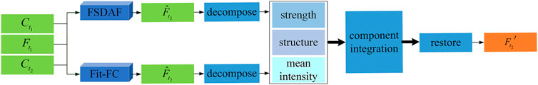
FIGURE 1. Flowchart of the proposed combination method.

An image x can be decomposed in the form of moments into three components, namely, strength, structure, and mean intensity,

$\begin{array}{cc}\hfill \mathbf{x}& ={‖\mathbf{x}-{\mu }_{\mathbf{x}}‖}_2\cdot \frac{\mathbf{x}-{\mu }_{\mathbf{x}}}{{‖\mathbf{x}-{\mu }_{\mathbf{x}}‖}_2}+{\mu }_{\mathbf{x}}\hfill \\ \hfill & ={‖\tilde{\mathbf{x}}‖}_2\cdot {\frac{\tilde{\mathbf{x}}}{‖\tilde{\mathbf{x}}‖}}_2+{\mu }_{\mathbf{x}}\hfill \\ \hfill & =c\cdot \mathbf{s}+l,\hfill \end{array}(17)$

where ${‖\cdot ‖}_2$ denotes the l₂ norm of a matrix, μ_x is the mean value, and $\tilde{\mathbf{x}}=\mathbf{x}-{\mu }_{\mathbf{x}}$ represents a zero-mean image. The scalar l = μ_x, $c={‖\tilde{\mathbf{x}}‖}_2$, and the unit-length matrix $\mathbf{s}=\tilde{\mathbf{x}}/‖\tilde{\mathbf{x}}‖$ roughly represent the strength component, structure component, and mean intensity component of x, respectively.

Each fused image can have its own components through decomposition. By integrating the components of multiple fusion results, the new components may outbreak the limitations of different fusion types. The merging strategy will be discussed in detail below.

The visibility of the image structure largely depends on the contrast, which is directly related to the intensity component. Generally, the higher the contrast, the better the visibility. However, too much contrast may lead to unrealistic representation of the image structure. All input images in this study are generated by spatiotemporal fusion algorithms, and their contrasts are usually higher than those of real images. This is reflected in the residual calculation of FSDAF and Fit-FC where stochastic errors are injected as well as details. Consequently, the image with the lowest contrast has the highest fidelity. Therefore, the desired contrast of the composite images is determined by the minimum contrast of all input images, that is, the fusion results of FSDAF and Fit-FC,

$\widehat{c}=\mathrm{m}\mathrm{i}\mathrm{n}\left(c_1,c_2\right)=\mathrm{m}\mathrm{i}\mathrm{n}\left({‖{\tilde{\mathbf{x}}}_1‖}_2,\Vert {\tilde{\mathbf{x}}}_2{\Vert }_2\right),(18)$

where ${\tilde{\mathbf{x}}}_1$ and ${\tilde{\mathbf{x}}}_2$ represent the zero-mean fusion images of FSDAF and Fit-FC, respectively.

The structure component is defined by the unit matrix s. It is expected that the structure of the fused image can represent the structures of all the input images effectively, which is calculated with the following:

$\widehat{\mathbf{s}}={\sum }_i{W}_i{\mathbf{s}}_i/{\sum }_i{W}_i,(19)$

where W_i is the weight to determine the contribution of the ith image by its structural component s_i.

To increase the contribution of higher-contrast images, a power-weighting function is given by the following:

$W_i={‖{\tilde{\mathbf{x}}}_i‖}_p,(20)$

where p ≥ 0 is a norm limited in 1, 2, or ∞.

The value of p is adaptive to the structure consistency of the input images, which is measured based on the degree of direction consistency R as

$R=‖{\sum }_i{\tilde{\mathbf{x}}}_i‖/{\sum }_i‖{\tilde{\mathbf{x}}}_i‖.(21)$

The norm p is empirically set to 1 when R ≤ 0.7, ∞ when R ≥ 0.98, and 2 otherwise.

The structural strategy is dedicated to the combination of FSDAF and Fit-FC. For the heterogeneous areas, Fit-FC predicts weak details, while the results of FSDAF are rich and relatively accurate. When the above method is used, the structure of FSDAF accounts for a large proportion. For the homogeneous landscapes, Fit-FC predicts fewer details in a more accurate way, while the results of FSDAF are richer but not accurate. In this case, the two images are mixed in a relatively similar ratio to achieve a tradeoff between detail and accuracy.

The intensity component can be estimated with weights as

$\widehat{l}={\sum }_i{w}_i{l}_i/{\sum }_i{w}_i.(22)$

Here, w_i is the weight normalized with the Gaussian function as given below:

$w_i=\exp \left(-\frac{{\left({\mu }_i-{\mu }_c\right)}^2}{2{\sigma }_i^2}\right),(23)$

where μ_i and ${\sigma }_i^2$ are the mean value and variance of the ith image, respectively. μ_c is a constant approaching the mid-intensity value. The typical value of μ_c is 0.5, which is far higher than the mean value of a linearly normalized remote sensing image for visual improvement.

After the combined values $\widehat{c}$, $\widehat{\mathbf{s}}$, and $\widehat{l}$ are calculated, the target image is restored with the following:

$\widehat{\mathbf{x}}=\widehat{c}\cdot \widehat{\mathbf{s}}+\widehat{l}.(24)$

The integration strategy is performed band by band, which requires the maximum and minimum normalization of all the input images in unified thresholds.

4 Experiment

4.1 Experimental Scheme

The datasets for validation are the Coleambally irrigation area (CIA) and Lower Gwydir Catchment (LGC) that were used in Emelyanova et al. (2013). CIA has 17 pairs of Landsat-7 ETM + and MODIS images, and LGC has 14 pairs of Landsat-5 TM and MODIS images. Four pairs of Landsat-8 images are also used for the spatiotemporal experiment, which were captured in November 2017 and December 2017. The path number is 121, and the row number is 41 and 43. These images have six bands, of which the blue, green, red, and near-infrared (NIR) bands are reconstructed. All images are cropped to the size of 1200 × 1200 at the center to avoid the outer blank areas. For the CIA and LGC datasets, four pairs of images were used for training and four pairs of images were used to validate the accuracy. For the Landsat-8 dataset, 2 pairs of images were used for training and the other 2 pairs of images were used to validate the accuracy. In each dataset, the two adjacent pairs of images are set as the known image pair and prediction image pair, respectively. The dates of the predicted images are marked in Tables 1–6.

TABLE 1

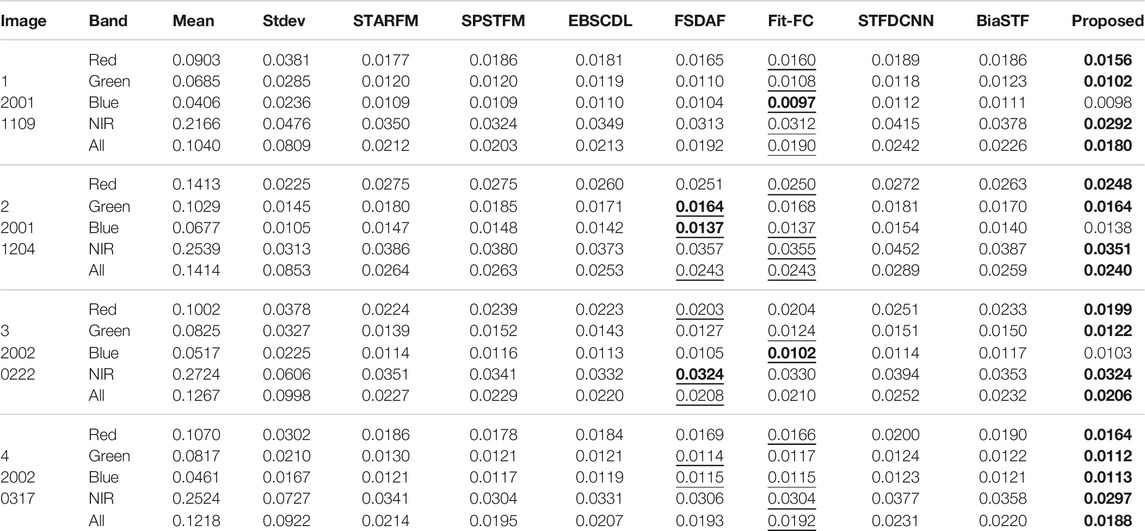
TABLE 1. RMSE evaluation of radiometric error for the CIA dataset.

To judge the effectiveness of the proposed method, some state-of-the-art algorithms are compared, including STARFM (Gao et al., 2006), SPSTFM (Huang and Song, 2012), EBSCDL (Wu et al., 2015a), FSDAF (Zhu et al., 2016), Fit-FC (Wang and Atkinson, 2018), STFDCNN (Song et al., 2018), and BiaSTF (Li et al., 2020a). STARFM and Fit-FC use linear weights. FSDAF is an unmixing-based method. SPSTFM and EBSCDL are based on the coupled dictionary learning. STFDCNN and BiaSTF were recently proposed that use the CNNs and deep learning.

The default parameter settings were kept for all competing algorithms. For STFDCNN, the SGD optimizer was used in the training, the batch size was set as 64, the training iterated 300 epochs with the learning rate of the first two layers set to 1 × 10⁻⁴ and the last layer to 1 × 10⁻⁵, and the training images were cropped into patches with a size of 64 × 64 for learning purposes. For BiaSTF, the Adam optimizer was used in the training by setting β₁ = 0.9, β₂ = 0.999, and ϵ = 10⁻⁸; the batch size was set as 64, the training iterated 300 epochs with the learning rate set as 1 × 10⁻⁴, and the training images were cropped into patches with a size of 128 × 128 for learning purposes. The experimental environment is listed in Table 7.

Metrics are used to evaluate the loss of radiation, the structure, and the spectrum. Root-mean-square-error (RMSE) measures the radiometric error. Structural similarity (SSIM) measures the similarity of contours and shapes. The Spectral Angle Mapper (SAM), Erreur Relative Globale Adimensionnelle de Synthese (ERGAS) (Du et al., 2007), and a Quaternion theory-based quality index (Q4) (Alparone et al., 2004) measure the spectral consistency. RMSE and SSIM are calculated band by band, while ERGAS and Q4 are calculated with the NIR, red, green, and blue bands as a whole. The ideal values are 1 for SSIM and Q4 while 0 for RMSE, SAM, and ERGAS.

4.2 Radiometric and Structural Assessment

RMSE and SSIM are calculated band by band. To save space, four fusion results are listed for each dataset, which are evaluated with RMSE in Tables 1–3, SSIM in Tables 4–6, SAM in Table 8, ERGAS in Table 9, and Q4 in Table 10. The best scores are marked in bold, and the better ones between scores of FSDAF and Fit-FC are underlined.

Table 1 shows the radiometric error of Landsat-7 reconstruction. It is clear that FSDAF and Fit-FC can produce more competitive results than dictionary learning– and deep learning–based methods. Compared with FSDAF, Fit-FC works better for image 1 but shows equal advantages for images 2, 3, and 4. The proposed method produces the least radiometric loss in majority cases.

The radiometric error of Landsat-5 is assessed in Table 2. It is observed that the performance of FSDAF, Fit-FC, and STFDCNN is accompanied with large fluctuation in image 3 due to the quick change caused by floods. Fit-FC ranks higher than FSDAF for the NIR band. STARFM, EBSCDL, and BiaSTF show better performance than SPSTFM. Again, the proposed method produces the least radiometric loss in most cases.

TABLE 2

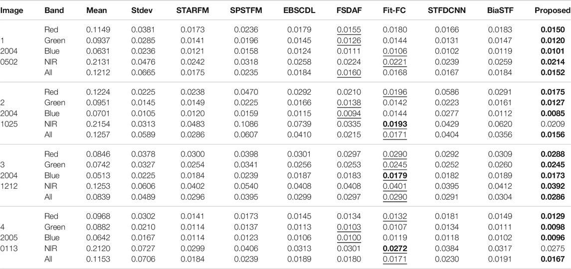
TABLE 2. RMSE evaluation of radiometric error for the LGC dataset.

The radiometric error of Landsat-8 is assessed in Table 3. The two dictionary-learning methods, SPSTFM and EBSCDL, perform well in the blue and NIR bands. Fit-FC performs poorly on image 43, making the proposed method slightly worse than FSDAF. It can also be seen that the method proposed in this study is suitable for the fusion of two results with little difference to produce a better result. When the two results differ greatly, the combination shows high stability.

TABLE 3

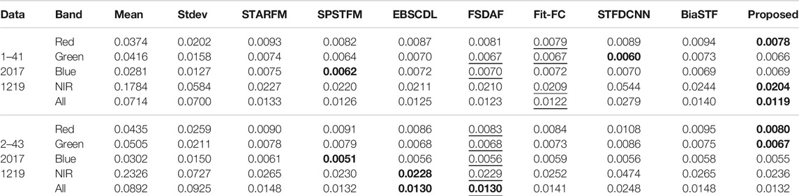
TABLE 3. RMSE evaluation of radiometric error for the Landsat-8 dataset.

The structural similarity is measured in Tables 4–6. The digital differences between algorithms are small. For Landsat-7 (Table 4), FSDAF shows strong superiority than Fit-FC, while the advantage is weak for image 2 of Landsat-5 (Table 5). STFDCNN and dictionary learning–based methods show good structural reconstruction for Landsat-7 and Landsat-8. For Landsat-5, STFDCNN works well for images 1 and 3 but poorly for image 2. The proposed method works steadily well in preserving good structures.

TABLE 4

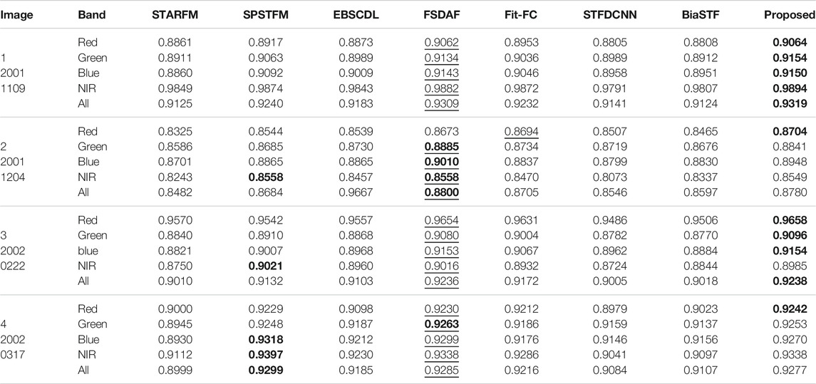
TABLE 4. SSIM evaluation of structural discrepancy for the CIA dataset.

TABLE 5

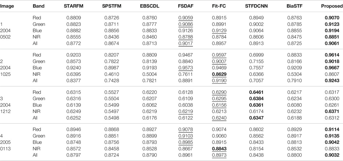
TABLE 5. SSIM evaluation of radiometric error for the LGC dataset.

TABLE 6

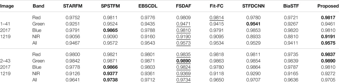
TABLE 6. SSIM evaluation of radiometric error for the Landsat-8 dataset.

TABLE 7

TABLE 7. Hardware and software for experiment.

4.3 Spectral Assessment

SAM is assessed in Table 8 with the NIR, red, green, and blue bands as a whole. SPSTFM works well for Landsat-8 but poor for Landsat-5. FSDAF and Fit-FC can produce better results for various datasets. The proposed method gives the best scores for the majority of images.

TABLE 8

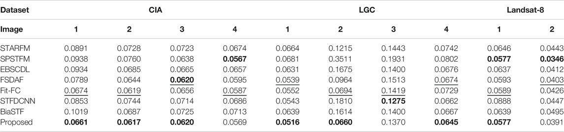
TABLE 8. SAM evaluation of spectral inconsistency.

ERGAS and Q4 for spectral assessment are calculated with the NIR, red, green, and blue bands as a whole. ERGAS is assessed in Table 9. The majority of the algorithms work well except for SPSTFM. FSDAF shows better performance than Fit-FC for Landsat-7 but poorer for Landsat-5. The proposed method gives the best scores for all images.

TABLE 9

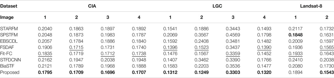
TABLE 9. ERGAS evaluation of spectral inconsistency.

Q4 is listed in Table 10 for spectral observation with the red, green, and blue bands as a whole. Images 2 and 3 of Landsat-5 are challenging due to the quick change of ground content, where dictionary-based and CNN-based methods produce much poor results. FSDAF and Fit-FC work well for most images. The proposed method shows competitive performance as it gives the best scores for the majority of images.

TABLE 10

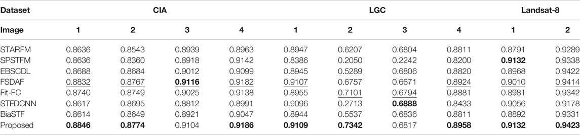
TABLE 10. Q4 evaluation of spectral inconsistency (R/G/B).

4.4 Visual Comparison

Four groups of images are demonstrated in Figures 2–5 for visual identification of the NIR, red, and green bands. All images are linearly stretched with the thresholds by which the brightest and darkest 2% pixels of the ground truth images are reassigned band by band. In this way, the color distortion can be read from the visually enhanced images directly. The manifested images in Figures 2, 3, 5 illustrate that FSDAF produces more details while Fit-FC fuses more consistent colors. Our method adopts both the advantages effectively to approach the true image. The flood area in Figure 4 shows that none of the algorithms can reconstruct the quick change in a large region yet despite the effort of FSDAF on changed landscapes.

FIGURE 2

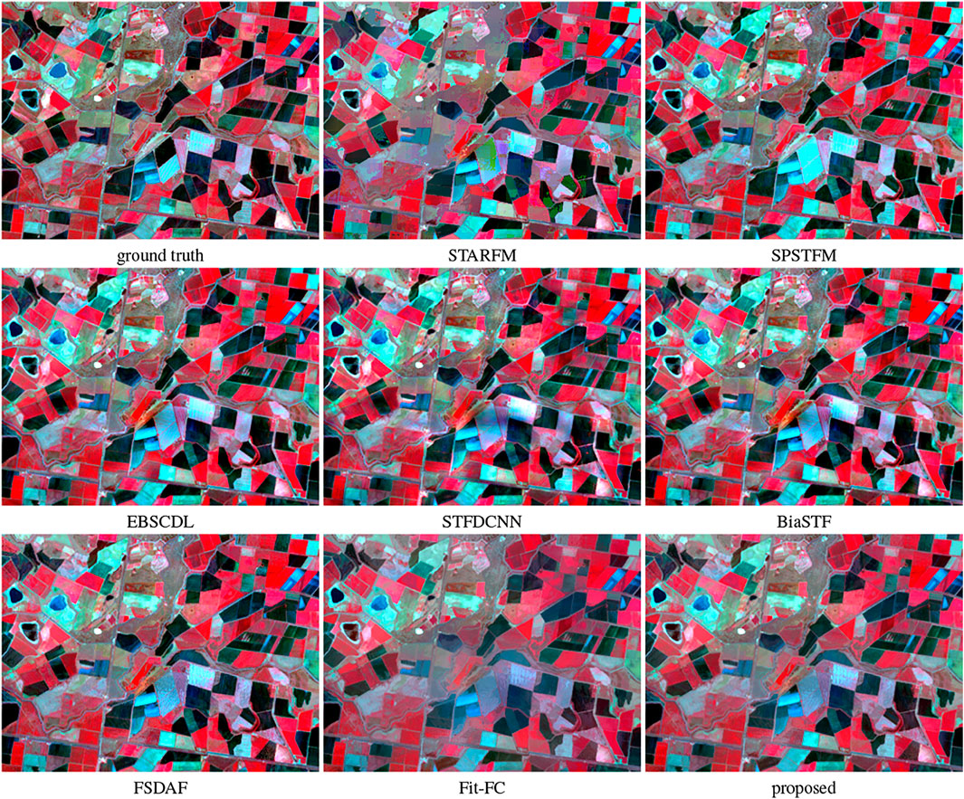
FIGURE 2. Manifestation of the small region of the NIR, red, and green bands of CIA image 1 for detail observation.

FIGURE 3

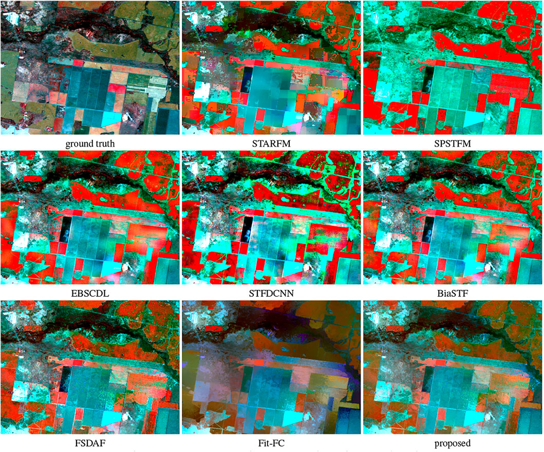
FIGURE 3. Manifestation of the small region of the NIR, red, and green bands of LGC image 2 for detail observation.

FIGURE 4

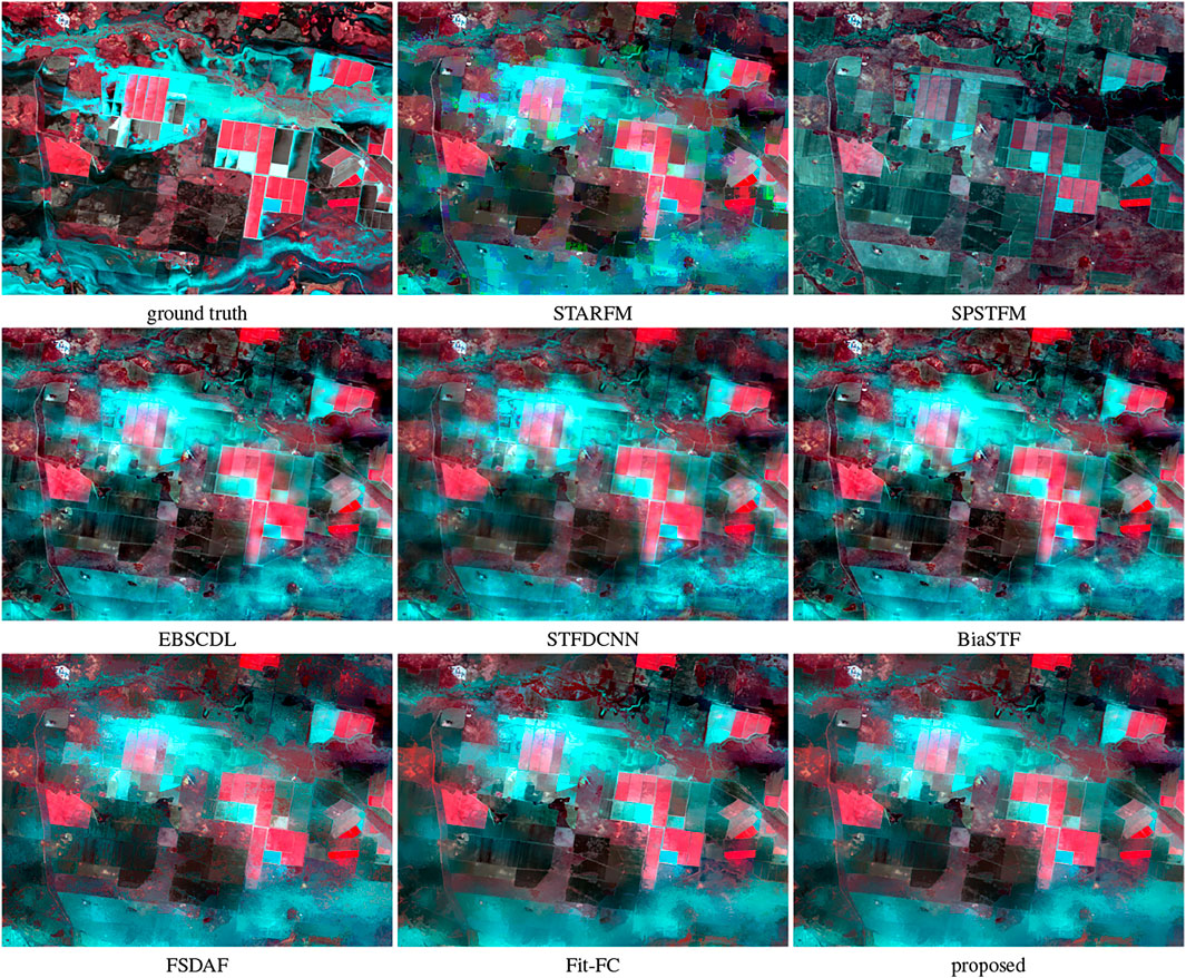
FIGURE 4. Manifestation of the large region of the NIR, red, and green bands of LGC image 3 for flood observation.

FIGURE 5

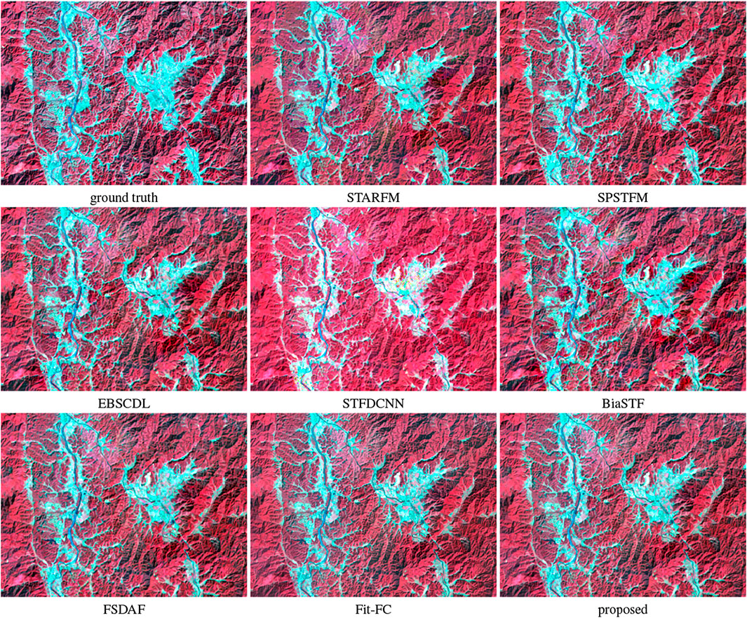
FIGURE 5. Manifestation of the small region of the NIR, red, and green bands of Landsat-8 image 1 for detail observation.

4.5 Computational Cost

The consumed time in a single prediction is recorded in Table 11, in which all the Python code used GPUs (nVidia 2080Ti) for acceleration. It is not fair to compare the time directly because the codes use various programming languages. For our method, the integration process takes only 6 s to combine the fusion results of FSDAF and Fit-FC. Since the fusion algorithms can work in a parallel way, the consumed time for the proposed method is recorded as the longest time plus the combination strategy.

TABLE 11

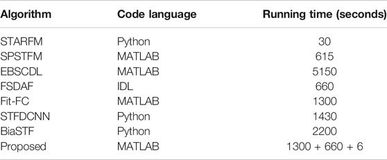
TABLE 11. Computational cost.

5 Discussion

The stability of our method is worthy of noting. On the one hand, derived from the excellent original methods, our synthetic method hits the highest score in most cases. By comparing the digital evaluation, it is concluded that the proposed method is usually better than the results of FSDAF and Fit-FC, which proves the complementarity indirectly. On the other hand, when our method fails to produce the best results, its score is close to the highest score.

The experiment shows that the proposed method may be improved. The RMSE comparison shows that Fit-FC is weakly better than FSDAF, but the SSIM comparison gives a contrary conclusion. Even though our proposed method is much effective, it does not make full use of the conclusion. To design a more feasible integration strategy, more tests are required to identify the unique advantages of spatiotemporal fusion algorithms, which are prevented in this study by the limited space.

For spatiotemporal fusion, there is no similar method focusing on integrating the fusion results for better performance. The only analogous method was proposed by Chen et al. (2020), who discussed the issue of data selection for performance improvement. Different kinds of algorithms have different advantages. Then, a good algorithm can design complex processes that incorporate multiple kinds for higher quality, or it can integrate the results through post-processing as the method in this article did. Intuitively, the idea in this article can be used for more remote sensing issues, such as pansharpening, denoising, inpainting, and so on.

The main disadvantage of the method is the increased time. As can be seen from Table 11, the post-processing time is very short so we have to run two or more different algorithms that extend the total time. This can be partly solved by launching algorithms in a parallel way. Then, the total time is constrained by the slowest algorithm.

The proposed method is usually not sensitive to the data quality of the input images. Some of the fusion results may be poor for specific images, while the proposed method tends to choose the best image block from multiple inputs. For them, the targeted selection of the fusion result, that is, the merger strategy, is the key. By performing this operation block by block, the quality of the whole image is improved.

6 Conclusion

Aiming at the insufficient stability of spatiotemporal fusion algorithms, this study proposes to make use of the complementarity of spatiotemporal fusion algorithms for better fusion results. An integration strategy is proposed for the images fused by FSDAF and Fit-FC. Their fusion results are decomposed into a strength component, a structure component, and a mean intensity component, which are packed to form a new fusion image.

The proposed method is tested on Landsat-5, Landsat-7, and Landat-8 images and compared with seven algorithms of four different types. The experimental results confirm the effectiveness of the spatial fusion strategy. The quantitative evaluation on radiometric, structural, and spectral loss shows that images produced by our method can reach or approach the optimal performance.

Data Availability Statement

Publicly available datasets were analyzed in this study. This data can be found here: https://data.csiro.au/collections/#collection/CIcsiro:5846v1 and https://data.csiro.au/collections/#collection/CIcsiro:5847v1.

Author Contributions

JW proposed the idea and wrote the paper. YM made the program and experiment. XH provided suggestions for data processing.

Funding

This paper was supported by the National Natural Science Foundation of China (No. 61860130) and the 03 Special and 5G Project of the Jiangxi Province (No. 20204ABC03A40).

Conflict of Interest

The authors declare that the research was conducted in the absence of any commercial or financial relationships that could be construed as a potential conflict of interest.

Publisher’s Note

All claims expressed in this article are solely those of the authors and do not necessarily represent those of their affiliated organizations, or those of the publisher, the editors, and the reviewers. Any product that may be evaluated in this article, or claim that may be made by its manufacturer, is not guaranteed or endorsed by the publisher.

References

Alparone, L., Baronti, S., Garzelli, A., and Nencini, F. (2004). A Global Quality Measurement of Pan-Sharpened Multispectral Imagery. IEEE Geosci. Remote Sens. Lett. 1, 313–317. doi:10.1109/lgrs.2004.836784

CrossRef Full Text | Google Scholar

Chen, Y., Cao, R., Chen, J., Zhu, X., Zhou, J., Wang, G., et al. (2020). A New Cross-Fusion Method to Automatically Determine the Optimal Input Image Pairs for Ndvi Spatiotemporal Data Fusion. IEEE Trans. Geosci. Remote Sens. 58, 5179–5194. doi:10.1109/tgrs.2020.2973762

CrossRef Full Text | Google Scholar

Choi, J. H., Elgendy, O. A., and Chan, S. H. (2019). Optimal Combination of Image Denoisers. IEEE Trans. Image Process. 28, 4016–4031. doi:10.1109/tip.2019.2903321

PubMed Abstract | CrossRef Full Text | Google Scholar

Dai, P., Zhang, H., Zhang, L., and Shen, H. (2018). “A Remote Sensing Spatiotemporal Fusion Model of Landsat and Modis Data via Deep Learning,” in IGARSS 2018 - 2018 IEEE International Geoscience and Remote Sensing Symposium, 7030–7033. doi:10.1109/igarss.2018.8518758

CrossRef Full Text | Google Scholar

Du, Q., Younan, N. H., King, R., and Shah, V. P. (2007). On the Performance Evaluation of Pan-Sharpening Techniques. IEEE Geosci. Remote Sens. Lett. 4, 518–522. doi:10.1109/lgrs.2007.896328

CrossRef Full Text | Google Scholar

Emelyanova, I. V., McVicar, T. R., Van Niel, T. G., Li, L. T., and van Dijk, A. I. J. M. (2013). Assessing the Accuracy of Blending Landsat-Modis Surface Reflectances in Two Landscapes with Contrasting Spatial and Temporal Dynamics: A Framework for Algorithm Selection. Remote Sens. Environ. 133, 193–209. doi:10.1016/j.rse.2013.02.007

CrossRef Full Text | Google Scholar

Fu, D., Chen, B., Wang, J., Zhu, X., and Hilker, T. (2013). An Improved Image Fusion Approach Based on Enhanced Spatial and Temporal the Adaptive Reflectance Fusion Model. Remote Sens. 5, 6346–6360. doi:10.3390/rs5126346

CrossRef Full Text | Google Scholar

Feng Gao, F., Masek, J., Schwaller, M., and Hall, F. (2006). On the Blending of the Landsat and Modis Surface Reflectance: Predicting Daily Landsat Surface Reflectance. IEEE Trans. Geosci. Remote Sens. 44, 2207–2218. doi:10.1109/tgrs.2006.872081

CrossRef Full Text | Google Scholar

Gevaert, C. M., and García-Haro, F. J. (2015). A Comparison of Starfm and an Unmixing-Based Algorithm for Landsat and Modis Data Fusion. Remote Sens. Environ. 156, 34–44. doi:10.1016/j.rse.2014.09.012

CrossRef Full Text | Google Scholar

Hilker, T., Wulder, M. A., Coops, N. C., Linke, J., McDermid, G., Masek, J. G., et al. (2009). A New Data Fusion Model for High Spatial- and Temporal-Resolution Mapping of forest Disturbance Based on Landsat and Modis. Remote Sens. Environ. 113, 1613–1627. doi:10.1016/j.rse.2009.03.007

CrossRef Full Text | Google Scholar

Huang, B., and Song, H. (2012). Spatiotemporal Reflectance Fusion via Sparse Representation. IEEE Trans. Geosci. Remote Sens. 50, 3707–3716. doi:10.1109/tgrs.2012.2186638

CrossRef Full Text | Google Scholar

Bo Huang, B., Juan Wang, J., Huihui Song, H., Dongjie Fu, D., and KwanKit Wong, K. (2013). Generating High Spatiotemporal Resolution Land Surface Temperature for Urban Heat Island Monitoring. IEEE Geosci. Remote Sens. Lett. 10, 1011–1015. doi:10.1109/lgrs.2012.2227930

CrossRef Full Text | Google Scholar

Li, X., Wang, L., Cheng, Q., Wu, P., Gan, W., and Fang, L. (2019). Cloud Removal in Remote Sensing Images Using Nonnegative Matrix Factorization and Error Correction. Isprs J. Photogramm. Remote Sens. 148, 103–113. doi:10.1016/j.isprsjprs.2018.12.013

CrossRef Full Text | Google Scholar

Li, Y., Li, J., He, L., Chen, J., and Plaza, A. (2020a). A New Sensor Bias-Driven Spatio-Temporal Fusion Model Based on Convolutional Neural Networks. Sci. China-Inform. Sci. 63. doi:10.1007/s11432-019-2805-y

CrossRef Full Text | Google Scholar

Li, Y., Wu, H., Li, Z.-L., Duan, S., and Ni, L. (2020b). “Evaluation of Spatiotemporal Fusion Models in Land Surface Temperature Using Polar-Orbiting and Geostationary Satellite Data,” in IGARSS 2020 - 2020 IEEE International Geoscience and Remote Sensing Symposium, 236–239. doi:10.1109/igarss39084.2020.9323319

CrossRef Full Text | Google Scholar

Liu, X., Deng, C., and Zhao, B. (2016). “Spatiotemporal Reflectance Fusion Based on Location Regularized Sparse Representation,” in 2016 IEEE International Geoscience and Remote Sensing Symposium (IGARSS), 2562–2565. doi:10.1109/igarss.2016.7729662

CrossRef Full Text | Google Scholar

Liu, P., Zhang, H., and Eom, K. B. (2017). Active Deep Learning for Classification of Hyperspectral Images. IEEE J. Sel. Top. Appl. Earth Observ. Remote Sens. 10, 712–724. doi:10.1109/jstars.2016.2598859

CrossRef Full Text | Google Scholar

Liu, X., Deng, C., Chanussot, J., Hong, D., and Zhao, B. (2019). Stfnet: A Two-Stream Convolutional Neural Network for Spatiotemporal Image Fusion. IEEE Trans. Geosci. Remote Sens. 57, 6552–6564. doi:10.1109/tgrs.2019.2907310

CrossRef Full Text | Google Scholar

Liu, Y., Xu, S., and Lin, Z. (2020). An Improved Combination of Image Denoisers Using Spatial Local Fusion Strategy. IEEE Access 8, 150407–150421. doi:10.1109/access.2020.3016766

CrossRef Full Text | Google Scholar

Song, H., and Huang, B. (2013). Spatiotemporal Satellite Image Fusion through One-Pair Image Learning. IEEE Trans. Geosci. Remote Sens. 51, 1883–1896. doi:10.1109/tgrs.2012.2213095

CrossRef Full Text | Google Scholar

Song, H., Liu, Q., Wang, G., Hang, R., and Huang, B. (2018). Spatiotemporal Satellite Image Fusion Using Deep Convolutional Neural Networks. IEEE J. Sel. Top. Appl. Earth Observ. Remote Sens. 11, 821–829. doi:10.1109/jstars.2018.2797894

CrossRef Full Text | Google Scholar

Tan, Z., Yue, P., Di, L., and Tang, J. (2018). Deriving High Spatiotemporal Remote Sensing Images Using Deep Convolutional Network. Remote Sens. 10, 1066. doi:10.3390/rs10071066

CrossRef Full Text | Google Scholar

Tan, Z., Di, L., Zhang, M., Guo, L., and Gao, M. (2019a). An Enhanced Deep Convolutional Model for Spatiotemporal Image Fusion. Remote Sens. 11, 2898. doi:10.3390/rs11242898

CrossRef Full Text | Google Scholar

Tan, Z. Q., Wang, X. L., Chen, B., Liu, X. G., and Zhang, Q. (2019b). Surface Water Connectivity of Seasonal Isolated Lakes in a Dynamic lake-floodplain System. J. Hydrol. 579, 13. doi:10.1016/j.jhydrol.2019.124154

CrossRef Full Text | Google Scholar

Tan, Z., Gao, M., Li, X., and Jiang, L. (2021). A Flexible Reference-Insensitive Spatiotemporal Fusion Model for Remote Sensing Images Using Conditional Generative Adversarial Network. IEEE Trans. Geosci. Remote Sens., 1–13. doi:10.1109/tgrs.2021.3050551

CrossRef Full Text | Google Scholar

Wang, Q., and Atkinson, P. M. (2018). Spatio-temporal Fusion for Daily Sentinel-2 Images. Remote Sens. Environ. 204, 31–42. doi:10.1016/j.rse.2017.10.046

CrossRef Full Text | Google Scholar

Wang, J., and Huang, B. (2017). A Rigorously-Weighted Spatiotemporal Fusion Model with Uncertainty Analysis. Remote Sens. 9, 990. doi:10.3390/rs9100990

CrossRef Full Text | Google Scholar

Wei, J., Wang, L., Liu, P., Chen, X., Li, W., and Zomaya, A. Y. (2017a). Spatiotemporal Fusion of Modis and Landsat-7 Reflectance Images via Compressed Sensing. IEEE Trans. Geosci. Remote Sens. 55, 7126–7139. doi:10.1109/tgrs.2017.2742529

CrossRef Full Text | Google Scholar

Wei, J., Wang, L., Liu, P., and Song, W. (2017b). Spatiotemporal Fusion of Remote Sensing Images with Structural Sparsity and Semi-coupled Dictionary Learning. Remote Sens. 9, 21. doi:10.3390/rs9010021

CrossRef Full Text | Google Scholar

Weng, Q., Fu, P., and Gao, F. (2014). Generating Daily Land Surface Temperature at Landsat Resolution by Fusing Landsat and Modis Data. Remote Sens. Environ. 145, 55–67. doi:10.1016/j.rse.2014.02.003

CrossRef Full Text | Google Scholar

Wu, M., Niu, Z., Wang, C., Wu, C., and Wang, L. (2012). Use of Modis and Landsat Time Series Data to Generate High-Resolution Temporal Synthetic Landsat Data Using a Spatial and Temporal Reflectance Fusion Model. J. Appl. Remote Sens. 6, 063507. doi:10.1117/1.jrs.6.063507

CrossRef Full Text | Google Scholar

Wu, B., Huang, B., and Zhang, L. (2015a). An Error-Bound-Regularized Sparse Coding for Spatiotemporal Reflectance Fusion. IEEE Trans. Geosci. Remote Sens. 53, 6791–6803. doi:10.1109/tgrs.2015.2448100

CrossRef Full Text | Google Scholar

Wu, M., Huang, W., Niu, Z., and Wang, C. (2015b). Generating Daily Synthetic Landsat Imagery by Combining Landsat and Modis Data. Sensors 15, 24002–24025. doi:10.3390/s150924002

PubMed Abstract | CrossRef Full Text | Google Scholar

Yong Xu, Y., Bo Huang, B., Yuyue Xu, Y., Kai Cao, K., Chunlan Guo, C., and Deyu Meng, D. (2015). Spatial and Temporal Image Fusion via Regularized Spatial Unmixing. IEEE Geosci. Remote Sens. Lett. 12, 1362–1366. doi:10.1109/lgrs.2015.2402644

CrossRef Full Text | Google Scholar

Zhang, W., Li, A., Jin, H., Bian, J., Zhang, Z., Lei, G., et al. (2013). An Enhanced Spatial and Temporal Data Fusion Model for Fusing Landsat and Modis Surface Reflectance to Generate High Temporal Landsat-like Data. Remote Sens. 5, 5346–5368. doi:10.3390/rs5105346

CrossRef Full Text | Google Scholar

Zhang, L., Liu, P., Zhao, L., Wang, G., Zhang, W., and Liu, J. (2021). Air Quality Predictions with a Semi-supervised Bidirectional Lstm Neural Network. Atmos. Pollut. Res. 12, 328–339. doi:10.1016/j.apr.2020.09.003

CrossRef Full Text | Google Scholar

Zhu, X., Chen, J., Gao, F., Chen, X., and Masek, J. G. (2010). An Enhanced Spatial and Temporal Adaptive Reflectance Fusion Model for Complex Heterogeneous Regions. Remote Sens. Environ. 114, 2610–2623. doi:10.1016/j.rse.2010.05.032

CrossRef Full Text | Google Scholar

Zhu, X., Helmer, E. H., Gao, F., Liu, D., Chen, J., and Lefsky, M. A. (2016). A Flexible Spatiotemporal Method for Fusing Satellite Images with Different Resolutions. Remote Sens. Environ. 172, 165–177. doi:10.1016/j.rse.2015.11.016

CrossRef Full Text | Google Scholar

Zhu, X., Cai, F., Tian, J., and Williams, T. K.-A. (2018). Spatiotemporal Fusion of Multisource Remote Sensing Data: Literature Survey, Taxonomy, Principles, Applications, and Future Directions. Remote Sens. 10, 527. doi:10.3390/rs10040527

CrossRef Full Text | Google Scholar

Zhukov, B., Oertel, D., Lanzl, F., and Reinhackel, G. (1999). Unmixing-based Multisensor Multiresolution Image Fusion. IEEE Trans. Geosci. Remote Sens. 37, 1212–1226. doi:10.1109/36.763276

CrossRef Full Text | Google Scholar

Zurita-Milla, R., Clevers, J., and Schaepman, M. E. (2008). Unmixing-based Landsat Tm and Meris Fr Data Fusion. IEEE Geosci. Remote Sens. Lett. 5, 453–457. doi:10.1109/lgrs.2008.919685

CrossRef Full Text | Google Scholar