
94% of researchers rate our articles as excellent or good
Learn more about the work of our research integrity team to safeguard the quality of each article we publish.
Find out more
ORIGINAL RESEARCH article
Front. Environ. Sci., 25 November 2021
Sec. Interdisciplinary Climate Studies
Volume 9 - 2021 | https://doi.org/10.3389/fenvs.2021.716968
This article is part of the Research TopicUrban Climate InformaticsView all 12 articles
Urban climate features, such as the urban heat island (UHI), are determined by various factors characterizing the modifications of the surface by the built environment and human activity. These factors are often attributed to the local spatial scale (hundreds of meters up to several kilometers). Nowadays, more and more urban climate studies utilize the concept of the local climate zones (LCZs) as a proxy for urban climate heterogeneity. However, for modern megacities that extend to dozens of kilometers, it is reasonable to suggest a significant contribution of the larger-scale factors to the temperature and UHI climatology. In this study, we investigate the contribution of local-scale and mesoscale driving factors of the nocturnal canopy layer UHI of the Moscow megacity in Russia. The study is based on air temperature observations from a dense network consisting of around 80 reference and more than 1,500 crowdsourced citizen weather stations for a summer and a winter season. For the crowdsourcing data, an advanced quality control algorithm is proposed. Based on both types of data, we show that the spatial patterns of the UHI are shaped both by local-scale and mesoscale driving factors. The local drivers represent the surface features in the vicinity of a few hundred meters and can be described by the LCZ concept. The mesoscale drivers represent the influence of the surrounding urban areas in the vicinity of 2–20 km around a station, transformed by diffusion, and advection in the atmospheric boundary layer. The contribution of the mesoscale drivers is reflected in air temperature differences between similar LCZs in different parts of the megacity and in a dependence between the UHI intensity and the distance from the city center. Using high-resolution city-descriptive parameters and different statistical analysis, we quantified the contributions of the local- and mesoscale driving factors. For selected cases with a pronounced nocturnal UHI, their respective contributions are of similar magnitude. Our findings highlight the importance of taking both local- and mesoscale effects in urban climate studies for megacities into account. Furthermore, they underscore a need for an extension of the LCZ concept to take mesoscale settings of the urban environment into account.
The urban heat island (UHI) is one of the most studied examples of inadvertent climate modification due to humans and refers to the fact that cities are almost always warmer than their natural surroundings (Oke et al., 2017; Stewart, 2019). UHIs affect urban dwellers in various (in)direct ways, e.g., by increased levels of heat risk/stress and heat-related mortality (Tan et al., 2010; Gabriel and Endlicher, 2011; Zemtsov et al., 2020), and are, thus, important to include in weather forecasts (Barlage et al., 2016; Baklanov et al., 2018; Rivin et al., 2020), climate-responsive urban planning (Svensson and Eliasson, 2002; Fernandez Milan and Creutzig, 2015; Emmanuel, 2021), and ecological and epidemiological applications (Gregg et al., 2003; Mironova et al., 2019; Brousse et al., 2020). UHIs are expressed at different vertical levels from subsurface soil temperatures to atmospheric boundary layer (ABL), yet the most studied and relevant for many applied tasks is a so-called canopy layer UHI, defined as the difference between the near-surface air temperatures below roof level (Oke et al., 2017). It is typically studied based on the screen level (1.5–2 m) temperature observations. Further in this paper, by UHI, we mean exactly the canopy layer UHI.
A distinctive feature of urban climates is their high spatial heterogeneity, determined by a variety of urban forms, land cover types, and anthropogenic activity on different spatial scales, and the complexity of the surface–atmosphere interaction in cities. The question of spatial scale is acknowledged as central in urban climate studies (Oke et al., 2017). It is important for observational data analysis and numerical modeling, for resolving the climatic heterogeneity in applied tasks, and for developing physically based urban climate models. However, while its importance has been recognized over decades of urban climate research (Stewart, 2019), specific contributions of processes at different spatial scales to certain urban climate phenomena remain vague.
Heterogeneity of urban forms and land cover types can be expressed on a wide range of spatial scales from micro- to mesoscale, each corresponding to typical horizontal length scales from meters to kilometers (Oke et al., 2017), and leading to scale-dependent urban climate phenomena (Pacifici et al., 2019). Among this range of scales, the so-called local scale (i.e., hundreds of meters to several kilometers) is considered to be especially relevant for UHI studies. At such scale, canopy layer air temperatures are directly influenced by their underlying surface properties (Stewart and Oke, 2012). In order to make urban climate studies more comparable and to facilitate metadata collection and description of measurement sites, Stewart and Oke (2012) developed the concept of local climate zones (LCZs), where LCZs are defined as regions of uniform surface cover, structure, material, and human activity that span hundreds of meters to several kilometers in horizontal scale. This concept classifies urban and rural environments according to local-scale surface cover, morphology, and human activities into 10 “built” and 7 “natural” classes, where each class has a set of characteristic parameter values (e.g., sky view factor, built-up surface fraction, and vegetation surface fraction). The body of literature using the LCZ concept is fast growing (Demuzere et al., 2021), highlighting the applicability of the concept in UHI studies and showing that different LCZs possess different air temperature regimes (see, e.g., Alexander and Mills, 2014; Fenner et al., 2014; Stewart et al., 2014; Skarbit et al., 2017; Beck et al., 2018a; Verdonck et al., 2018; Milošević et al., 2021). Despite the fact that a microscale temperature heterogeneity can still be observed within the same LCZs or neighborhoods (Ellis et al., 2015; Leconte et al., 2015; Quanz et al., 2018; Shi et al., 2018; Pacifici et al., 2019), the LCZ system is widely acknowledged as a global standard for urban temperature studies (Stewart and Oke, 2012; Jiang et al., 2021).
Beyond the LCZ framework, several studies attempted to explain UHI spatial structures through local-scale variability of land cover and morphology properties. Several studies revealed dependencies between the UHI intensity and land cover parameters such as green area fraction, artificial cover fraction, and building area fraction (Bottyán et al., 2005; van Hove et al., 2015; Scott et al., 2017). More advanced statistical models were developed to predict UHI intensity, e.g., for Portland, United States (Hart and Sailor, 2009), Wroclaw, Poland (Szymanowski and Kryza, 2009), Rotterdam, Netherlands (Heusinkveld et al., 2014), and 35 European cities (Sangiorgio et al., 2020), using several local-scale parameters as predictors, e.g., building and road density, surface roughness, albedo, greenery, and anthropogenic heat flux.
Local-scale variations in surface cover and morphology determine modifications of the surface–atmosphere interaction regime within the surface layer of the atmosphere with a depth of a few tens of meters (Oke et al., 2017). However, for medium-sized cities and even more so for megacities, the influence of the various neighborhoods on the atmosphere is accumulated and further transformed over tens of kilometers, resulting in modifications of the whole ABL and the development of the phenomena induced by the city as a whole. According to the classification of atmospheric processes by scale (Orlanski, 1975), such phenomena can be considered as mesoscale processes. The examples of urban-induced mesoscale atmospheric phenomena include the ABL heat island with a vertical extent of hundreds of meters (Bornstein, 1968; Oke, 1995; Wouters et al., 2013; Lokoshchenko et al., 2016; Varentsov et al., 2018), urban plumes (Clarke, 1969; Wang et al., 2020), urban-induced modifications of regional circulation (Lemonsu and Masson, 2002; Varentsov et al., 2018), and deep convection systems, precipitation, and cloudiness (Bornstein and Lin, 2000; Dixon and Mote, 2003; Han et al., 2014).
The urban-caused mesoscale phenomena not only involve the “bottom–up” urban forcing affecting the ABL and lower troposphere but also provide “top–down” impacts on the canopy layer climate and spatial patterns of the UHI. The latter is clearly expressed, e.g., in the UHI advection to the leeward side of the city and its neighboring rural areas, as reported both by modeling (Zhang et al., 2011; Heaviside et al., 2015) and observation-based (Bassett et al., 2016; Bassett et al., 2017) studies. On a quasi-climatic approximation, heat advection from varied wind directions, together with diffusion, and mixing by mesoscale circulations, are expected to smooth the local-scale thermal heterogeneity of the urban environment, and to make the climate of the given site sensitive to surface parameters outside its local-scale neighborhood. Mesoscale smoothing is expected to be among the factors establishing the known logarithmic relation between UHI intensity and city size or population (Oke, 1973; Zhou et al., 2017; Li et al., 2020).
Despite the obvious contribution of mesoscale processes to the development of urban climates, they are often ignored in spatially resolving UHI studies, including those ones aimed to predict urban temperature heterogeneity based on land cover parameters (Hart and Sailor, 2009; Szymanowski and Kryza, 2009; Heusinkveld et al., 2014). A few counterexamples include the studies for Leipzig, Germany (Franck et al., 2013), Detroit, United States, (Oswald et al., 2012), and several French (Gardes et al., 2020) and Dutch (Theeuwes et al., 2017) cities, where the authors attempted to account for both local-scale parameters and the meso-climatic features of the area through the distance from the city center and large water bodies. On the other hand, local-scale factors may be also ignored. For example, the recent work by Manoli et al. (2019) continues to explore the varying UHI intensity with population size, yet others believe this coarse-grained approach is insufficient and inappropriate, even as a first-order guidance approach (Martilli et al., 2020).
The abovementioned contradictions about the scale-dependent drivers of the UHI may, in part, be attributed to the lack of detailed observational data. To resolve urban climate phenomena with observations, high-density observational networks with stations installed in various settings are required. Such networks are deployed in different cities, e.g., in Birmingham, United Kingdom (Chapman et al., 2015); Dijon, France (Richard et al., 2018); Szeged, Hungary (Lelovics et al., 2014); and Novi Sad, Serbia (Milošević et al., 2021); see review in Muller et al. (2013) for further examples. However, the large majority of global cities do not possess such networks, as they are costly to install and maintain over longer periods of time (Muller et al., 2013).
In recent years, the use of nontraditional and opportunistic-sensing technologies in meteorological and climatological research, such as smartphones (Overeem et al., 2013b; Mass and Madaus, 2014; Droste et al., 2017), cars (Haberlandt and Sester, 2010; Mahoney and O’Sullivan, 2013; Bartos et al., 2019), commercial microwave links (Messer et al., 2006; Zinevich et al., 2009; Overeem et al., 2013a; Chwala and Kunstmann, 2019), wrist-mounted wearables (Nazarian et al., 2020), and privately owned citizen weather stations (CWSs), e.g., Wolters and Brandsma (2012), Bell et al. (2015), de Vos et al. (2017), Meier et al. (2017), Fenner et al. (2019), Droste et al. (2020), and Mandement and Caumont (2020), have shown to provide additional and reliable information, thus, highlighting a multitude of possible applications in research and beyond (de Vos et al., 2019; Nipen et al., 2020). To study urban air temperatures and the UHI effect, data from CWSs have been used in a variety of studies (Steeneveld et al., 2011; Chapman et al., 2017; Fenner et al., 2017; de Vos et al., 2020; Feichtinger et al., 2020; Venter et al., 2020; Vulova et al., 2020), focusing on different cities. One major advantage of CWSs over traditional meteorological stations is their large number within a single city (Meier et al., 2017). Further, CWSs are located in a large variety of micro- and local-scale settings, distributed all over a city region (Fenner et al., 2017), thus, detecting the spatial heterogeneity of urban air temperatures.
Decades of research provide evidence that local- and mesoscale processes are important drivers shaping urban thermal environment. This is relevant both for specific atmospheric processes as well as the scales of the surface heterogeneity influencing the climate of specific site, which are referred to as drivers in this study. However, it remains largely unknown to what extent both scales determine the spatial heterogeneity of urban air temperatures. To disentangle these two influencing spatial scales, this study focuses on the megacity of Moscow, Russia. The city is a perfect testbed for this question since it is located far away from the sea and has no significant topography, ruling out these geographic controls on the formation of its UHI. Furthermore, a large set of near-surface observations is available from both professionally maintained stations and amateur CWSs in a large variety of meso- and local-scale settings. The overall aim of the study is to investigate the respective contributions of meso- and local-scale heterogeneity of urban surface to the nighttime canopy layer UHI in Moscow.
Moscow is the most populous Russian and European megacity (55.75°N, 37.62°E) with a population of approximately 17 million people (considering the whole urban agglomeration) (Cox, 2017). The actual area of the city (excluding the suburbs and satellite cities) is about 1,000 km2. Moscow has a temperate humid and moderately continental climate (Dfb in the Köppen–Geiger climate classification, Beck et al., 2018b) with an annual mean air temperature of 5.8°C, and mean June and January temperatures of 19.2°C and −6.5°C, respectively (values are given for VDNKh weather station, Figure 1, for the period 1981–2010). Due to the cold winters, Moscow is known as one of the coldest megacities of the world. The intense urban-induced meteorological effects of Moscow are easy to detect against the homogeneous rural surroundings. The city experienced an increasing UHI intensity over the last decades (Kislov et al., 2017), with a present-day annual mean UHI intensity of 2°C, peaking to more than 10°C during calm and clear nights (Lokoshchenko, 2014; Lokoshchenko, 2017). Recently, Moscow served as a testbed for a series of high-resolution urban climate modeling studies with the COSMO model (Varentsov et al., 2017; Varentsov et al., 2019; Garbero et al., 2021), revealing persistent urban-induced mesoscale effects in the lower atmosphere (Varentsov et al., 2018) and high sensitivity of the simulated UHI to the spatial patterns of the urban canopy parameters (Varentsov et al., 2020b). Nonetheless, despite the numerous previous studies, the spatial patterns of the Moscow UHI and their physical drivers have not been systematically analyzed yet.
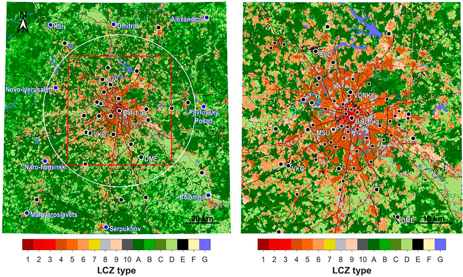
FIGURE 1. Local climate zone map from Varentsov et al. (2020b) and reference stations. The white circle in the left subplot depicts the study area involved in further statistical analysis, and the red box shows the smaller area shown in detail in the right subplot and used in the following maps. Circle markers indicate location of reference weather stations (WSs), and square markers indicate location of reference automatic air-quality stations (AAQSs, more info below). Nine WSs used to define mean background temperature are highlighted by blue.
This study focuses on an area centered around the city center of Moscow with a 60-km radius, thereby including Moscow itself, its suburbs, and satellite cities, yet not including the medium-sized cities around Moscow that are separated from the megacity by wide countryside areas (Figure 1).
We use regular observations from a dense reference network (hereafter referred to as REF) consisting of weather stations (WSs) of the Russian hydrometeorological service (Roshydromet) and automatic air-quality stations (AAQS) of Mosecomonitoring, the official environmental monitoring service of Moscow. The WSs provide the most reliable screen-level (1.5–2 m above the ground) air temperature observations according to the standards of the World Meteorological Organization (WMO). Yet, only a few WSs are available in urbanized areas: the Balchug WS in the city center, the meteorological observatory of the Lomonosov Moscow State University (MSU), VDNKh WS in an urban park, and several WSs in the suburbs. AAQSs cover the city with a denser network (Figure 1) but provide less accurate meteorological data. Meteorological observations by AAQSs do not comply with the WMO standards, e.g., the sensors are located at a height of 2 m above roofs of metal containers and 4 m above the ground. Previous studies showed that AAQS air temperature measurements may be biased during daytime. However, daily mean and nighttime temperatures are accurate enough for spatially explicit UHI studies (Varentsov et al., 2019).
We use REF air temperature data on a one-hourly temporal resolution with instantaneous values at the full hour to be consistent with the temporal resolution of the CWS data (see next subsection Citizen weather stations). The data were downsampled from the original 10- and 20-min resolutions of WSs and AAQSs, respectively. For a few WSs where only three-hourly observations are available, missing one-hourly temperature values were gap filled based on existing three-hourly values and one-hourly values for the nearest WSs, where they are available. In total, we use data from up to 42 WSs and up to 40 AAQSs (the actual number of stations varies due to data availability for the considered periods).
Crowdsourced air temperature data from CWSs of the “Netatmo” company (https://www.netatmo.com/en-us/weather) were acquired using the application programming interface (API) provided by the company (https://dev.netatmo.com/apidocumentation/weather). A full description of the device itself and the data acquisition, i.e., crowdsourcing, is given in Meier et al. (2017); a brief summary is given in the following. The device consists of an indoor and an outdoor module. From the latter, air temperature and relative humidity data can be acquired via the API. The specified accuracy for the air temperature sensor is ± 0.3 K in the range –40°C–65°C. Each CWS takes measurements approximately every 5 min, data are then automatically uploaded to the server of the company via WiFi connection. Netatmo data for the study area was collected at an hourly resolution (instantaneous values) using the workflow as described in Meier et al. (2017).
Netatmo CWSs provide uncertified observations, which can be misrepresentative for many reasons. For example, outdoor modules may be installed directly at walls or even inside buildings (Meier et al., 2017). Beyond these extreme cases, other typical ways of CWS installation could, nonetheless, be different from standards of meteorological observations, such as observations on balconies or below trees.
Previous studies have already shown the opportunity to filter out misrepresentative and faulty data using quality-control (QC) algorithms. Here, we developed a QC algorithm based on ideas from previous studies (Meier et al., 2017; Napoly et al., 2018) with some modifications, which allows to exploit the high number of reference observations in the Moscow region (Figure 1).
The preprocessing step, L0, removes CWSs with the same location (assuming that the location was wrongly defined by using the IP address; Meier et al., 2017). The following three steps, L1–L3, depend on statistics calculated over a period Δt = 14 days before the i-th moment for which the QC is applied. L1 is passed if the missing data ratio for the j-th CWS over the Δt period is lower than a threshold (Rgaps = 0.5). L2 is passed when the temperature mean value
This approach rejects CWSs if the outdoor module is located indoors and partially eliminates cases when the outdoor module is not shaded properly. The L3 step checks the Pearson correlation coefficient
Finally, a fifth step (L5) is added to remove too high spatial variability among closely located CWSs within a 3-km distance, following the idea of a “buddy check” from Båserud et al. (2020) and Nipen et al. (2020). The criteria for the L5 step for the temperature value for j-th CWS at i-th moment is based on its deviation from the mean value over the neighboring CWS:
where
For comparison with this new QC scheme, the raw CWS data were also filtered according to the “CrowdQC” procedures until level O1 (Grassmann et al., 2018; Napoly et al., 2018). Based on evaluation of the quality-controlled CWS data against closely located REF sites, we found that the proposed algorithm noticeably decreases the CWS errors with respect to unfiltered data and performs even better than CrowdQC, but passes slightly less data (see Supplementary S2 for details).
The quality-controlled CWS data is still not free from uncertainties, associated with the height of a CWS installation above the ground. CWSs may be installed at different heights, including the upper floors of high-rise buildings, which is far away from the standards of the WMO. Unfortunately, no methods of identification for the installation height of the CWS have been proposed so far. However, we assume that CWSs are typically installed below roof level and characterize the temperature of typically well-mixed air within the urban canopy and, hence, could be used to study the canopy layer UHI studies as already shown, e.g., in Fenner et al. (2017), Meier et al. (2017), Napoly et al. (2018), and Feichtinger et al. (2020).
Based on availability of REF and CWS data, as well as on weather conditions, we selected the periods of winter 2018/2019 (December and January) and summer 2019 (May and June) for our study. During the two winter months Moscow experienced low temperatures with a strong cold wave at the end of January 2019 (Figure 2A). May and June 2019 experienced warm weather that was favorable for UHI development, while July and August 2019 were cold, rainy, and unfavorable for UHI appearance. Therefore, we did not include July and August 2019 in the analyzed summer period.
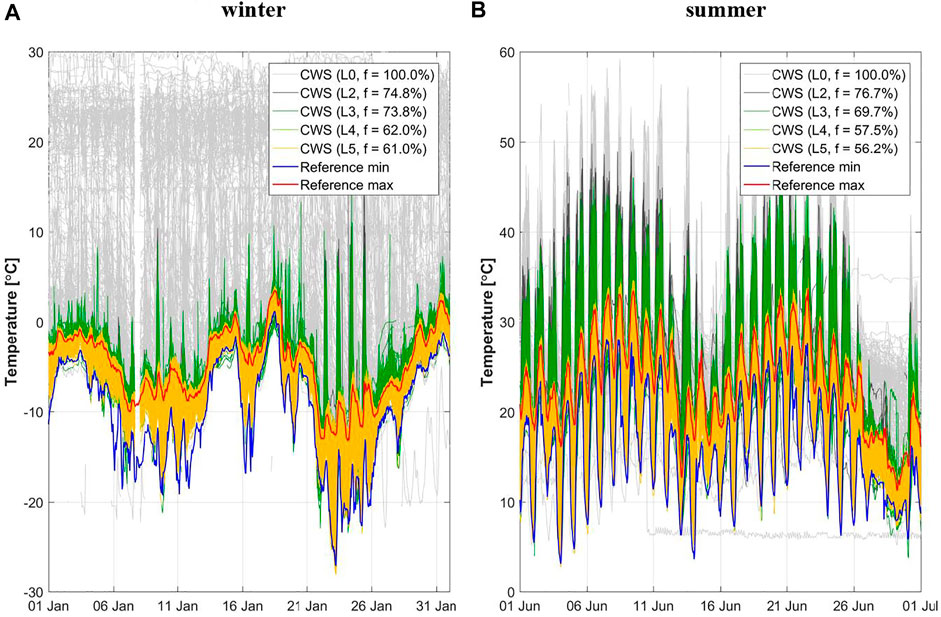
FIGURE 2. Air temperature in the study region for January 2019 (A) and June 2019 (B) for citizen weather station (CWS) data and reference observations. Quality control (QC) levels L0–L5 refer to the data after each respective level of quality control for CWS data. In the legend,
In the selected winter and summer periods, CWS data were collected from, respectively, 1,646 and 1,673 unique CWSs. Raw CWS data included numerous artifacts, which are typical for Netatmo temperature readings according to previous studies: unrealistically high daytime temperatures due to overheating of the unshaded outdoor modules by direct sunlight and unrealistic temperatures without expected diurnal variations for the CWSs placed somewhere indoors instead of outdoors (Meier et al., 2017; Napoly et al., 2018). The proposed QC algorithm successfully filters out such artifacts, which decreases the amount of individual temperature readings by 39% in winter and 44% in summer (Figure 2).
To analyze the spatial structure of the UHI and the factors of its formation in a quasi-climatological approximation, we sampled a selection of summer and winter cases characterized by intense UHIs. UHI intensity (
where
We used
As expected for cases with pronounced UHI, the sampled cases are characterized by generally calm weather conditions with a near-surface wind speed lower than 3 m/s and generally low low-level cloudiness (see Supplementary Figure S3 for details). Wind direction during the sampled cases is not homogeneous but is still quite diverse (Supplementary Figure S3.1), so we deem it acceptable for a coarse quasi-climatic approximation.
For the final analyses, we considered only reference stations and CWSs with a ratio of missed or QC-filtered values over all cases <25%, resulting in a total of 477 and 500 CWSs, and 67 and 61 REF sites within the study area, for winter and summer, respectively. The remaining stations were gap filled using a regression-based algorithm adopted after Tardivo and Berti (2012) to obtain continuous and homogeneous time series. Each individual gap for a specific station was filled based on a multiple linear regression using air temperature observations at neighboring stations as predictors (for each station, three to five neighboring stations were used that provided the best regression result). Regression coefficients were derived based on the data before and after each individual gap, separately for each hour of the day. When applying gap filling for CWS data, we only used REF data as predictors.
For each station, we calculated the mean air temperature over the selected summer or winter cases. To exclude a larger-scale spatial temperature gradient from our analysis, a two-dimensional latitude–longitude mean temperature trend was identified based on the observations at rural WSs for a larger area (within 300 km around Moscow) and subtracted from the mean temperatures. Finally, we calculated the mean
To characterize the heterogeneity of the underlying surface properties, our study combined two popular approaches, namely, the LCZ classification (Stewart and Oke, 2012) and independent quantitative estimation of city-descriptive parameters. The LCZ map for the Moscow region (Figure 1) is available from Varentsov et al. (2020b) at a 100-m spatial resolution. It was created based on training areas selected by Samsonov and Trigub (2018) and post-processed using a Gaussian kernel majority filter (Demuzere et al., 2020).
Each observation site (WS, AAQS, or CWS) was assigned to an LCZ class based on a majority filter applied for a circle with a 250-m radius around each site as suggested in Fenner et al. (2017). An important but nontrivial component of the LCZ assignment procedure is to detect the measurement sites surrounded by heterogeneous LCZ coverage and to exclude them from further analyses. Fenner et al. (2017) proposed to consider sites only if the LCZ for the central pixel of the kernel is equal to the major LCZ of the kernel and that this LCZ covers ≥80% of the area of the kernel. However, applying the same criteria for Moscow resulted in losing a high number of stations from both REF and CWS networks. We found that a lot of sites were excluded in cases where they are surrounded by two or more relatively similar LCZs. For example, a site may be surrounded by mixed open mid- and high-rise buildings, classified into LCZs 4 (open high-rise) and 5 (open mid-rise), or by low-rise private houses surrounded by vegetation classified as LCZs 6 (open low-rise) and 9 (sparsely built). To avoid such data loss, we proposed a procedure of LCZ assignment that accounts for the similarity between surrounding LCZs. For a kernel where the i-th LCZ occupies the largest area fraction
where
Based on the proposed approach, we considered a site to be in quasi-homogenous local-scale surroundings if the area fraction of the modal LCZ of the kernel is >0.5, and the similarity-weighted area fraction is >0.75. Otherwise, the station was excluded from the LCZ-dependent analyses. Additionally, and in contrast to the LCZ assignment procedure from Fenner et al. (2017), we do not use a condition that the LCZ for the nearest pixel of a station has to correspond to the modal LCZ, since the location of the stations are not always known with enough precision.
On top of the LCZ-based approach, several city-descriptive parameters were sourced from OpenStreetMap data, Sentinel-2 images, and Copernicus Global Land Cover (CGLC) data, following Samsonov and Varentsov (2020). Based on the literature review, we selected the following parameters that are commonly used as predictors for
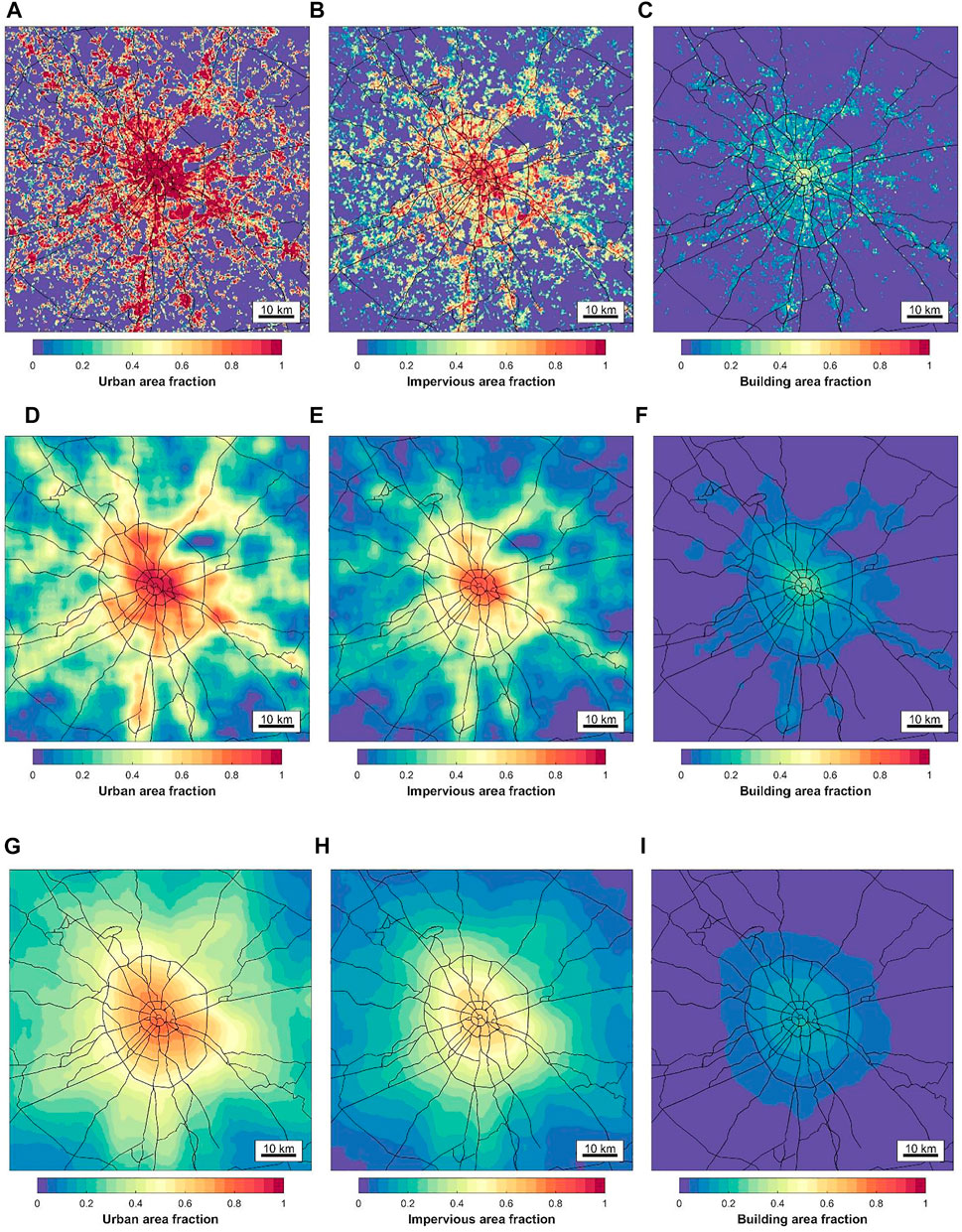
FIGURE 3. Spatial distribution of city-descriptive parameters
The central hypothesis of our study is that the
• LCZ-dependent analysis. This analysis focuses on the intra- and inter-LCZ variability of
• Simple correlation analysis. This analysis focuses on the relationships between
• Regression analysis with local-scale and mesoscale predictors. Based on the central hypothesis of our study, we propose to predict the observed
• As local-scale predictors
• Regression analysis with multi-scale predictors. Assuming that an MLR model with predictors of only two scales may be oversimplified and, therefore, skew the results, additional analyses are performed using an MLR model simultaneously involving predictors
• To avoid appearance of meaningless negative values of
Figure 4 shows the spatial distribution of the
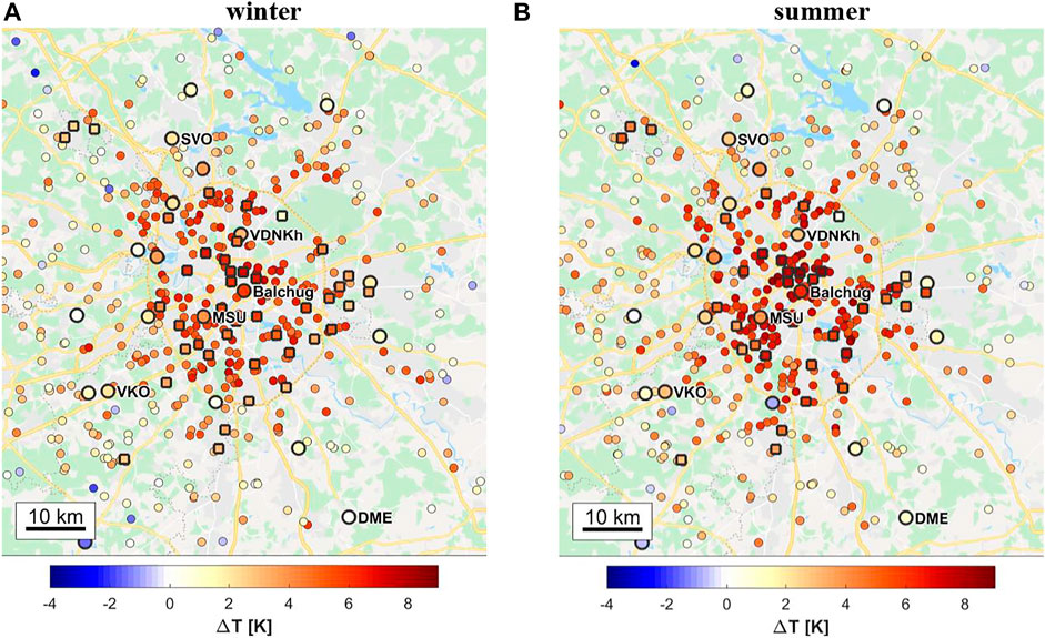
FIGURE 4. Spatial patterns of the mean urban heat island (UHI) intensity
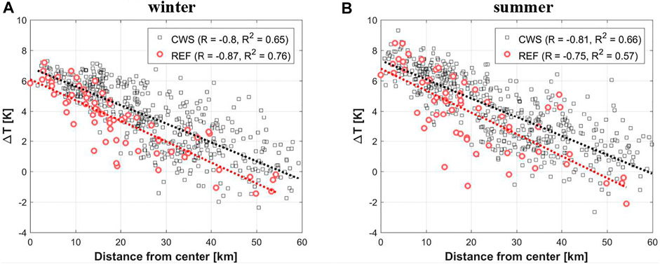
FIGURE 5. Dependence between UHI intensity
Figure 6 displays ΔT for each station, grouped by LCZ type. Intra-LCZ variability of air temperature and thus also
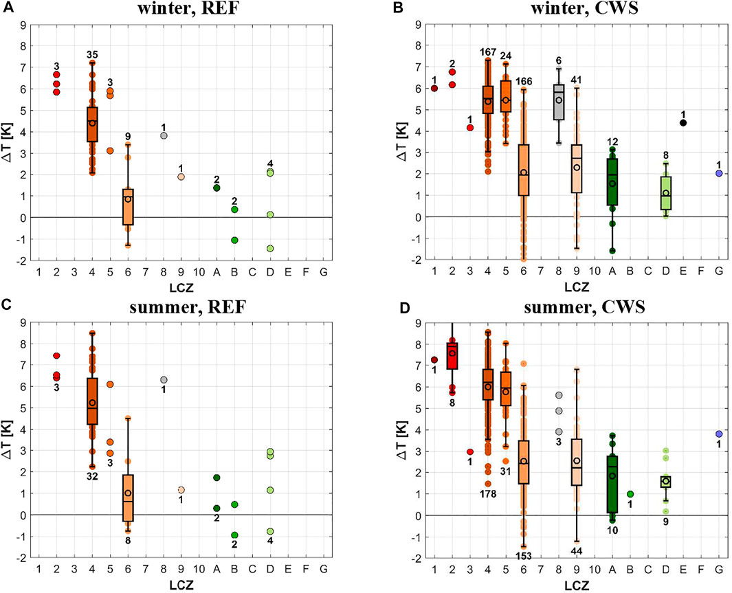
FIGURE 6. Boxplots representing the dependence between UHI intensity ΔT and LCZ type for winter (A, B) and summer (C, D) based on reference (A, C) and CWS (B, D) observations. Digits in the plots indicate the number of reference stations or CWSs related to specific LCZ types.
Comparing mean
To further investigate the intra-LCZ variability of ΔT seen in Figure 6, mean
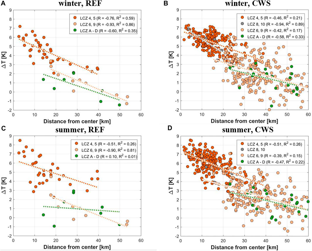
FIGURE 7. Dependence between UHI intensity
These LCZ-dependent results are, to some extent, sensitive to the thresholds used in the procedure of LCZ assignment for REF and CWS sites (see the Local climate zones and city-descriptive parameters section). Nevertheless, the key results and conclusions do not change (not shown).
Within a framework of simple correlation analysis, we analyzed correlations between
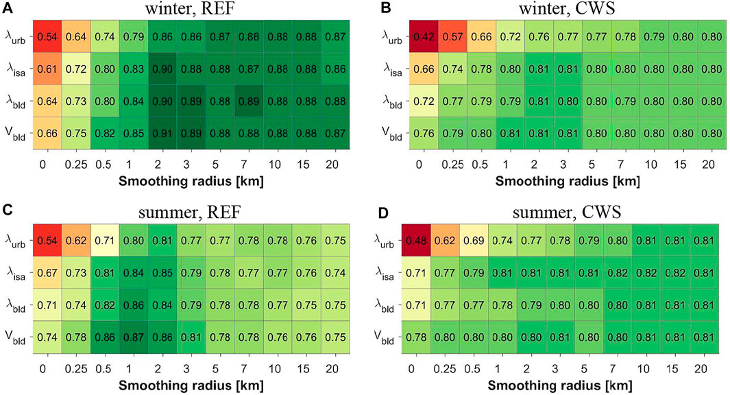
FIGURE 8. Spearman correlation coefficients, calculated between UHI intensity and selected city-descriptive parameters, smoothed with different radii for winter (A, B) and summer (C, D) periods, REF (A, C), and CWS (B, D) data. Zero radius means using the values on the original 250-m grid. The colors of the cells correspond to the values.
Results of the simple correlation analysis may be misinformative due to cross-correlation between city-descriptive parameters, smoothed with different radii. For example, the correlation coefficient between
Table 1 presents the results for the five combinations of predictors with the highest
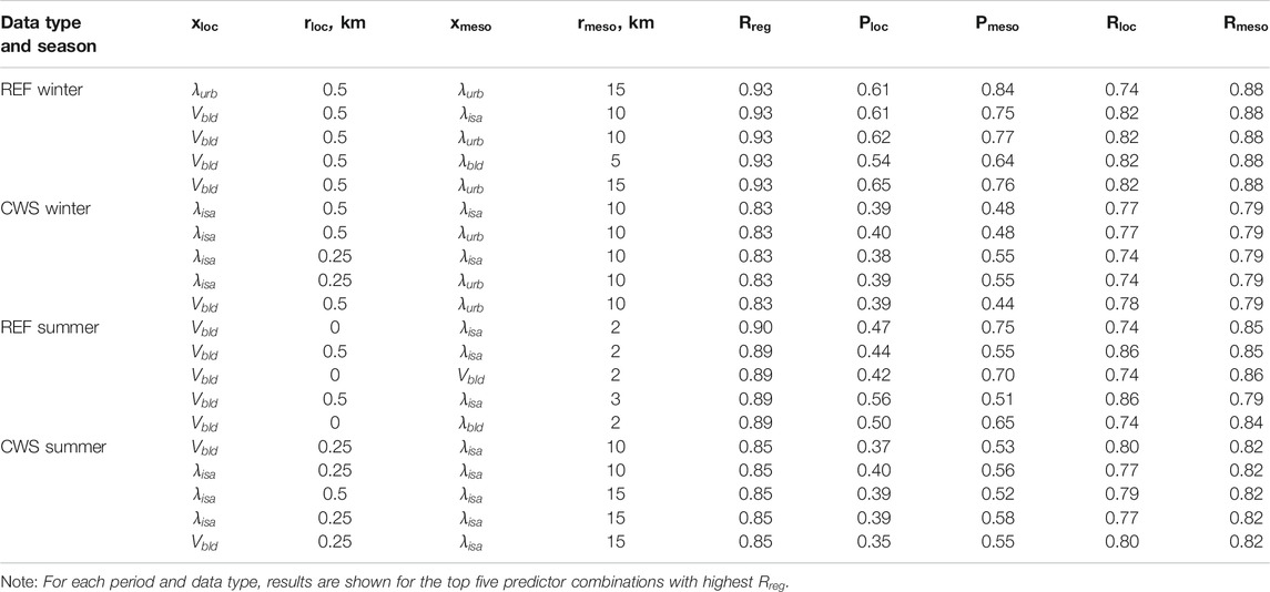
TABLE 1. Results of the multiple linear regression predicting of the summer and winter urban heat island (UHI) intensity based on reference network (REF) and citizen weather station (CWS) data.
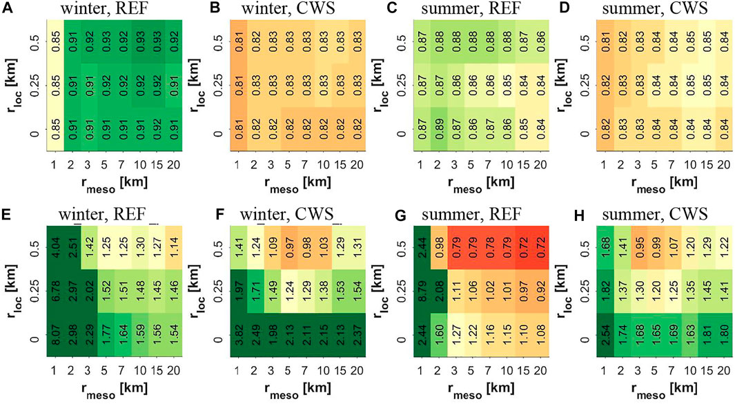
FIGURE 9. Values of
MLR models with multi-scale predictors, constructed as described by Eq. 3 in the Analysis strategy section, allow to compare the contribution of the specific scales of the surface heterogeneity to the observed UHI. Figure 10 shows the relative weights of predictors with different smoothing radius, averaged over the top 25% of predictor combinations among the randomly generated ensemble of 1,000 members. Despite the differences between plots for REF and CWS data, both networks demonstrate consistent patterns indicating the major contribution of the scales corresponding to
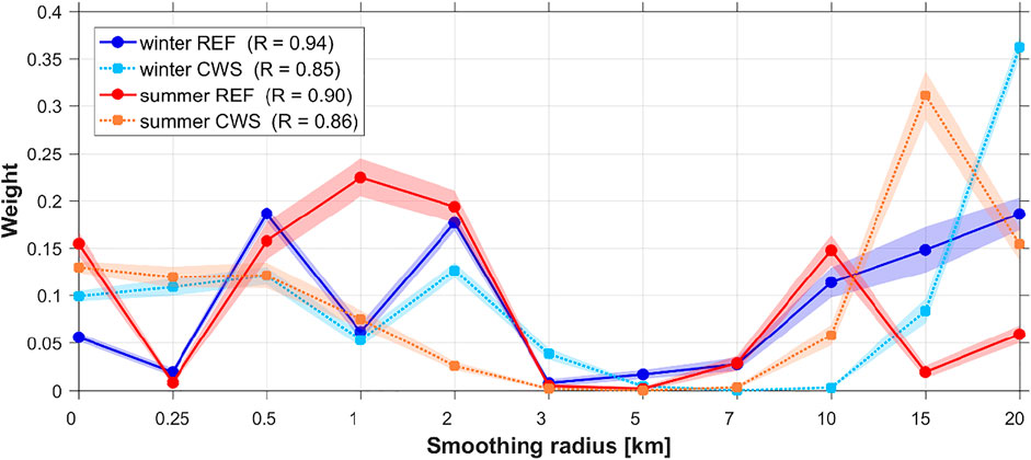
FIGURE 10. Mean relative weights of predictors, smoothed with different radii, in the multi-scale MLR model, averaged over best 25% of predictor combinations in randomly generated ensemble.
The UHI has been studied for decades, and it is one of the clearest examples of inadvertent climate modification due to humans (Oke et al., 2017). Land cover properties are known to play a crucial role in its development, yet the role of their spatial heterogeneity at various spatial scales remains unclear. The current study addresses this issue by linking the latter to the observed nocturnal canopy layer UHI of Moscow. Our results thereby provide a systematic understanding of the spatial scales affecting the UHI of a megacity.
The identified spatial patterns of the canopy layer UHI of Moscow are consistent with studies for other cities. As found by other studies focusing on LCZs and their thermal regimes (Stewart et al., 2014; Fenner et al., 2017; Skarbit et al., 2017; Beck et al., 2018a; Verdonck et al., 2018; Kwok et al., 2019; Milošević et al., 2021), we revealed a dependence between ΔT and LCZ type (Figure 6). The highest temperatures are found for densely built compact LCZs (1–3), which are warmer than open high-/mid-rise LCZs (4, 5), which again are warmer than low-rise residential areas (LCZ 6, 9) and natural LCZs. At the same time, intra-LCZ variability is comparable or even higher than inter-LCZ differences, especially for the most frequent LCZs in the study area (4, 6, and 9), which is consistent with previous studies (Leconte et al., 2015; Fenner et al., 2017; Skarbit et al., 2017; Quanz et al., 2018; Shi et al., 2018; Kwok et al., 2019).
Meanwhile, we obtained a strong negative correlation (
In order to explore the impacts of the land cover heterogeneity of different scales on the UHI spatial patterns, we suggest a novel approach based on a set of the city-descriptive parameters, defined on a 250-m grid, and further smoothed with several radii (
The presence of two dominant ranges of spatial scales suggests their connection with different physical processes. The contribution of scales with
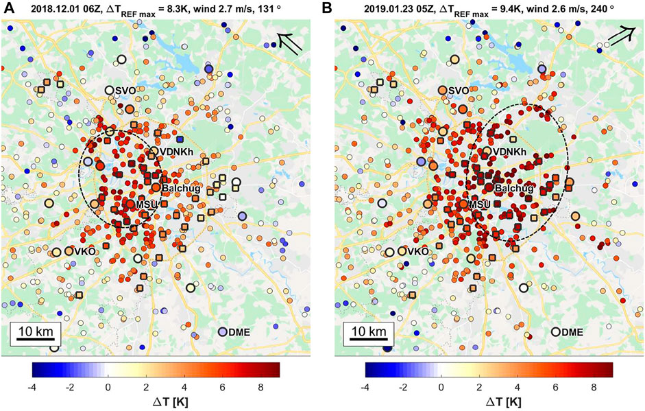
FIGURE 11. Spatial patterns of UHI intensity ΔT for two specific winter cases demonstrating an UHI shift to the leeward side of the city by south-easterly (A) and south-westerly (B) winds. Symbols are similar to Figure 4. The arrow in the top right corner shows the 10-m wind direction according to ERA5 reanalysis. The dotted line indicates the area with maximum ΔT. Digits in the caption indicate date and time, maximum ΔT according to REF data, ERA5 wind speed and direction.
The range of contributing scales with
In order to relate the contributing spatial scales revealed in our analysis to the heterogeneity of the LCZ classes in Moscow, we estimated the typical surface area size of homogenous LCZ patches. For this, we applied the “circle-based region width estimation” method (Samsonov et al., 2019) that assigns—to each pixel inside an LCZ patch—a characteristic radius. That radius corresponds to the largest circle covering the pixel without intersecting other LCZ classes (Supplementary Figure S5.1). Analyzing these radii grouped by LCZ class within the study area indicates that the typical LCZ class radius (mean or median) does not exceed 500 m for all LCZs, and is <300 m for all urban LCZs except 2 and 4 (Supplementary Figure S5.2). Such values are noticeably smaller than the range of 1–2 km, which provide significant contribution to the spatial UHI patterns (Figure 10). Hence, the range of contributing scales with
Based on dense reference and crowdsourced air temperature observations, we analyzed linkages between the nocturnal canopy layer UHI of Moscow and the land cover heterogeneity on different spatial scales, ranging from a few hundred meters to tens of kilometers. Land cover properties were described using the local climate zone (LCZ) classification and specific city-descriptive parameters, derived on a 250-m grid and smoothed with different radii (
Our results underscore that the thermal environment in Moscow is influenced by the heterogeneity of land cover properties on different scales, including local scale (a few hundred meters,
Our results recommend considering the mesoscale heterogeneity of land cover properties alongside the local-scale heterogeneity in urban climate studies and practical applications, especially for large cities. Our findings are especially relevant for statistical modeling of the urban thermal environment. It can be expected that the use of predictors reflecting mesoscale heterogeneity of land cover properties will improve the accuracy of temperature mapping for urban areas. Our results are also relevant for urban planning, since they underline the impact of local changes in specific areas (e.g., new urban developments) to its neighborhood on a mesoscale.
In order to assess the robustness of our findings, we propose the following research directions for follow-up studies:
• The proposed hypothesis should be tested for other cities, including more complex geographic controls, and for longer periods, since the sampling size in our study is relatively small, especially for winter. Moreover, the presented results are valid only for nocturnal cases with a pronounced UHI signature. Different patterns of air temperature may be expected during daytime and should be further investigated.
• Further studies are needed for deeper understanding of the physical processes beyond the revealed local-scale and mesoscale drivers. Yet, our study is based on a coarse-grained approach that analyzes the influencing scales of land cover heterogeneity through spatial smoothing of the city-descriptive parameters. Our results allow only suggesting about the physical processes responsible for such smoothing. More detailed and reliable knowledge may be gained based on high-resolution numerical simulations with mesoscale models, coupled to urban canopy schemes. Such modeling seems to be the only way to comprehensively analyze the interaction between UHI and atmospheric processes at different scales and different vertical levels from the surface up to the ABL.
• Despite the overall consistent results from the CWS and REF data, further research is needed to understand differences between the two types of stations, particularly regarding their spatial representativeness. Differences in the setup of the stations likely affect results regarding the contribution of scales; yet to what extent is not understood.
• Follow-up studies could explore the use of machine learning (ML) techniques that are already used to study and predict UHI spatial patterns (Straub et al., 2019; Gardes et al., 2020; Vulova et al., 2020). Simultaneously, existing ML-based techniques could be improved by considering the mesoscale heterogeneity of the urban environment.
• Additional attention should be paid to the scale smaller than the local scale, i.e., the microscale, which is ignored in our study. Yet, studies have shown that there is microscale variability within LCZs or neighborhoods, even of similar local-scale characteristic (see, e.g., Heusinkveld et al., 2014; Ellis et al., 2015; Leconte et al., 2015; Quanz et al., 2018; Shi et al., 2018; and Pacifici et al., 2019). Such an intra-LCZ variability is expected due to microscale variations in surface cover and morphology, exposure of the sensors, and anthropogenic heat sources. In the case of CWS, one can argue that due to their non-standard setup, the microscale influence is more pronounced than for reference observations (Fenner et al., 2017). This may explain the higher correlation coefficient for the CWS data without smoothing (
• In the end, our study highlights that further research is needed to systematically understand the contribution of spatial scales in urban thermal climate investigations across geographic and climatic regions, and cultures. This could lead to a possible extension of the LCZ concept to take mesoscale settings of the urban environment into account, further enhancing communication and reporting on the UHI effect throughout the scientific literature.
The raw data supporting the conclusion of this article will be made available by the authors, without undue reservation.
MV, DF, and FM proposed the concept of the study. DF and FM collected the CWS data. MD developed the LCZ map. TS developed the dataset with city-descriptive parameters and performed addition calculations with the LCZ map. MV collected the reference data, performed the bulk of the data analysis, and prepared the figures. MV, DF, and MD wrote the paper. All authors participated in the discussions and editing.
Processing and analysis of the observational data performed by MV was supported by the Russian Ministry of Education and Science, agreement no. 075-15-2021-574. The development of the city-descriptive datasets performed by TS and MV was supported by the Russian Ministry of Education and Science as part of the program of the Moscow Center for Fundamental and Applied Mathematics under agreement no. 075-15-2019-1621. Development of QC algorithm for CWS data was partially supported by the Interdisciplinary Scientific and Educational School of Moscow University «Brain, Cognitive Systems, Artificial Intelligence». Regression analysis of the linkages between UHI intensity and spatial predictors performed by MV was supported by the Russian Science Foundation, project no. 19-77-30012. Development of the impervious surface area fraction dataset and paper preparation was supported by the RUDN University Strategic Academic Leadership Program. The contributions of MD and DF were conducted in the context of project ENLIGHT, funded by the German Research Foundation (DFG) under grant no. 437467569. We acknowledge support by the German Research Foundation and the Open Access Publication Fund of TU Berlin for APC payment.
The authors declare that the research was conducted in the absence of any commercial or financial relationships that could be construed as a potential conflict of interest.
All claims expressed in this article are solely those of the authors and do not necessarily represent those of their affiliated organizations, or those of the publisher, the editors, and the reviewers. Any product that may be evaluated in this article, or claim that may be made by its manufacturer, is not guaranteed or endorsed by the publisher.
We thank all the citizens who make their Netatmo weather data publicly available. The authors are especially grateful to administration and staff of Hydrometeorological Research Center of Russian Federation, meteorological observatory of the Lomonosov Moscow State University and Budgetary Environmental Protection Institute “Mosecomonitoring” for providing the data of reference meteorological observations used in the study.
The Supplementary Material for this article can be found online at: https://www.frontiersin.org/articles/10.3389/fenvs.2021.716968/full#supplementary-material
Alexander, P., and Mills, G. (2014). Local Climate Classification and Dublin's Urban Heat Island. Atmosphere 5, 755–774. doi:10.3390/atmos5040755
Baklanov, A., Grimmond, C. S. B., Carlson, D., Terblanche, D., Tang, X., Bouchet, V., et al. (2018). From Urban Meteorology, Climate and Environment Research to Integrated City Services. Urban Clim. 23, 330–341. doi:10.1016/j.uclim.2017.05.004
Barlage, M., Miao, S., and Chen, F. (2016). Impact of Physics Parameterizations on High-Resolution Weather Prediction over Two Chinese Megacities. J. Geophys. Res. Atmos. 121, 4487–4498. doi:10.1002/2015JD024450
Bartos, M., Park, H., Zhou, T., Kerkez, B., and Vasudevan, R. (2019). Windshield Wipers on Connected Vehicles Produce High-Accuracy Rainfall Maps. Sci. Rep. 9, 170. doi:10.1038/s41598-018-36282-7
Båserud, L., Lussana, C., Nipen, T. N., Seierstad, I. A., Oram, L., and Aspelien, T. (2020). TITAN Automatic Spatial Quality Control of Meteorological In-Situ Observations. Adv. Sci. Res. 17, 153–163. doi:10.5194/asr-17-153-2020
Bassett, R., Cai, X., Chapman, L., Heaviside, C., Thornes, J. E., Muller, C. L., et al. (2016). Observations of Urban Heat Island Advection from a High-Density Monitoring Network. Q. J. R. Meteorol. Soc. 142, 2434–2441. doi:10.1002/qj.2836
Bassett, R., Cai, X., Chapman, L., Heaviside, C., and Thornes, J. E. (2017). The Effects of Heat Advection on UK Weather and Climate Observations in the Vicinity of Small Urbanized Areas. Boundary-layer Meteorol. 165, 181–196. doi:10.1007/s10546-017-0263-0
Bechtel, B., Demuzere, M., Sismanidis, P., Fenner, D., Brousse, O., Beck, C., et al. (2017). Quality of Crowdsourced Data on Urban Morphology—The Human Influence Experiment (HUMINEX). Urban Sci. 1, 15. doi:10.3390/urbansci1020015
Bechtel, B., Demuzere, M., and Stewart, I. D. (2020). A weighted accuracy measure for land cover mapping: Comment on johnson et al. local climate zone (LCZ) map accuracy assessments should account for land cover physical characteristics that affect the local thermal environment. remote sens 11, 2420. doi:10.3390/rs12111769
Beck, C., Straub, A., Breitner, S., Cyrys, J., Philipp, A., Rathmann, J., et al. (2018a). Air Temperature Characteristics of Local Climate Zones in the Augsburg Urban Area (Bavaria, Southern Germany) under Varying Synoptic Conditions. Urban Clim. 25, 152–166. doi:10.1016/j.uclim.2018.04.007
Beck, H. E., Zimmermann, N. E., McVicar, T. R., Vergopolan, N., Berg, A., and Wood, E. F. (2018b). Present and Future Köppen-Geiger Climate Classification Maps at 1-km Resolution. Sci. Data 5, 1–12. doi:10.1038/sdata.2018.214
Bell, S., Cornford, D., and Bastin, L. (2015). How Good Are Citizen Weather Stations ? Addressing a Biased Opinion. Weather 70, 75–84. doi:10.1002/wea.2316
Bornstein, R. D. (1968). Observations of the Urban Heat Island Effect in New York City. J. Appl. Meteorol. 7, 575–582. doi:10.1175/1520-0450(1968)007<0575:OOTUHI>2.0.CO;2
Bornstein, R., and Lin, Q. (2000). Urban Heat Islands and Summertime Convective Thunderstorms in Atlanta: Three Case Studies. AtmosEnviron 34, 507–516. doi:10.1016/S1352-2310(99)00374-X
Bottyán, Z., Kircsi, A., Szegedi, S., and Unger, J. (2005). The Relationship between Built-Up Areas and the Spatial Development of the Mean Maximum Urban Heat Island in Debrecen, Hungary. Int. J. Climatol. 25, 405–418. doi:10.1002/joc.1138
Brousse, O., Georganos, S., Demuzere, M., Dujardin, S., Lennert, M., Linard, C., et al. (2020). Can We Use Local Climate Zones for Predicting Malaria Prevalence across Sub-saharan African Cities. Environ. Res. Lett. 15, 124051. doi:10.1088/1748-9326/abc996
Chapman, L., Bell, C., and Bell, S. (2017). Can the Crowdsourcing Data Paradigm Take Atmospheric Science to a New Level? A Case Study of the Urban Heat Island of London Quantified Using Netatmo Weather Stations. Int. J. Climatol. 37, 3597–3605. doi:10.1002/joc.4940
Chapman, L., Muller, C. L., Young, D. T., Warren, E. L., Grimmond, C. S. B., Cai, X. M., et al. (2015). The birmingham Urban Climate Laboratory: An Open Meteorological Test Bed and Challenges of the Smart City. Bull. Am. Meteorol. Soc. 96, 1545–1560. doi:10.1175/BAMS-D-13-00193.1
Chwala, C., and Kunstmann, H. (2019). Commercial Microwave Link Networks for Rainfall Observation: Assessment of the Current Status and Future Challenges. WIREs Water 6, 1–20. doi:10.1002/wat2.1337
Clarke, J. F. (1969). Nocturnal Urban Boundary Layer over Cincinnati, Ohio. Mon. Weather Rev. 97, 582–589. doi:10.1175/1520-0493(1969)097<0582:nubloc>2.3.co;2
Cox, W. (2017). Demographia World Urban Areas. Belleville, Illinois: World Agglomerations. 13th Annua. Available at: http://www.demographia.com/db-worldua.pdf.
de Vos, L., Leijnse, H., Overeem, A., and Uijlenhoet, R. (2017). The Potential of Urban Rainfall Monitoring with Crowdsourced Automatic Weather Stations in Amsterdam. Hydrol. Earth Syst. Sci. 21, 765–777. doi:10.5194/hess-21-765-2017
de Vos, L. W., Droste, A. M., Zander, M. J., Overeem, A., Leijnse, H., Heusinkveld, B. G., et al. (2020). Hydrometeorological Monitoring Using Opportunistic Sensing Networks in the Amsterdam Metropolitan Area. Bull. Am. Meteorol. Soc. 101, E167–E185. doi:10.1175/BAMS-D-19-0091.1
de Vos, L. W., Leijnse, H., Overeem, A., and Uijlenhoet, R. (2019). Quality Control for Crowdsourced Personal Weather Stations to Enable Operational Rainfall Monitoring. Geophys. Res. Lett. 46, 8820–8829. doi:10.1029/2019GL083731
Demuzere, M., Hankey, S., Mills, G., Zhang, W., Lu, T., and Bechtel, B. (2020). Combining Expert and Crowd-Sourced Training Data to Map Urban Form and Functions for the continental US. Sci. Data 7, 1–13. doi:10.1038/s41597-020-00605-z
Demuzere, M., Kittner, J., and Bechtel, B. (2021). LCZ Generator: A Web Application to Create Local Climate Zone Maps. Front. Environ. Sci. 9. doi:10.3389/fenvs.2021.637455
Dienst, M., Lindén, J., and Esper, J. (2018). Determination of the Urban Heat Island Intensity in Villages and its Connection to Land Cover in Three European Climate Zones. Clim. Res. 76, 1–15. doi:10.3354/cr01522
Dienst, M., Lindén, J., Saladié, Ò., and Esper, J. (2019). Detection and Elimination of UHI Effects in Long Temperature Records from Villages – A Case Study from Tivissa, Spain. Urban Clim. 27, 372–383. doi:10.1016/j.uclim.2018.12.012
Dixon, P. G., and Mote, T. L. (2003). Patterns and Causes of Atlanta’s Urban Heat Island–Initiated Precipitation. J. Appl. Meteorol. 42, 1273–1284. doi:10.1175/1520-0450(2003)042<1273:pacoau>2.0.co;2
Droste, A. M., Heusinkveld, B. G., Fenner, D., and Steeneveld, G. J. (2020). Assessing the Potential and Application of Crowdsourced Urban Wind Data. Q. J. R. Meteorol. Soc. 146, 2671–2688. doi:10.1002/qj.3811
Droste, A. M., Pape, J. J., Overeem, A., Leijnse, H., Steeneveld, G. J., Van Delden, A. J., et al. (2017). Crowdsourcing Urban Air Temperatures through Smartphone Battery Temperatures in São Paulo, Brazil. J. Atmos. Ocean. Technol. 34, 1853–1866. doi:10.1175/JTECH-D-16-0150.1
Ellis, K. N., Hathaway, J. M., Mason, L. R., Howe, D. A., Epps, T. H., and Brown, V. M. (2015). Summer Temperature Variability across Four Urban Neighborhoods in Knoxville, Tennessee, USA. Theor. Appl. Climatol. 127, 701–710. doi:10.1007/s00704-015-1659-8
Emmanuel, R. (2021). Urban Microclimate in Temperate Climates: a Summary for Practitioners. Build. Cities 2, 402–410. doi:10.5334/bc.109
Feichtinger, M., de Wit, R., Goldenits, G., Kolejka, T., Hollósi, B., Žuvela-Aloise, M., et al. (2020). Case-study of Neighborhood-Scale Summertime Urban Air Temperature for the City of Vienna Using Crowd-Sourced Data. Urban Clim. 32, 1–12. doi:10.1016/j.uclim.2020.100597
Fenner, D., Holtmann, A., Meier, F., Langer, I., and Scherer, D. (2019). Contrasting Changes of Urban Heat Island Intensity during Hot Weather Episodes. Environ. Res. Lett. 14, 124013. doi:10.1088/1748-9326/ab506b
Fenner, D., Meier, F., Bechtel, B., Otto, M., and Scherer, D. (2017). Intra and Inter ‘local Climate Zone’ Variability of Air Temperature as Observed by Crowdsourced Citizen Weather Stations in Berlin, Germany. Meteorol. Z. 26, 525–547. doi:10.1127/metz/2017/0861
Fenner, D., Meier, F., Scherer, D., and Polze, A. (2014). Spatial and Temporal Air Temperature Variability in Berlin, Germany, during the Years 2001-2010. Urban Clim. 10, 308–331. doi:10.1016/j.uclim.2014.02.004
Fernandez Milan, B., and Creutzig, F. (2015). Reducing Urban Heat Wave Risk in the 21st century. Curr. Opin. Environ. Sustain. 14, 221–231. doi:10.1016/j.cosust.2015.08.002
Franck, U., Kruger, M., Schwarz, N., Grossmann, K., Roder, S., and Schlink, U. (2013). Heat Stress in Urban Areas: Indoor and Outdoor Temperatures in Different Urban Structure Types and Subjectively Reported Well-Being during a Heat Wave in the City of Leipzig. Meteorol. Z. 22, 167–177. doi:10.1127/0941-2948/2013/0384
Gabriel, K. M. A., and Endlicher, W. R. (2011). Urban and Rural Mortality Rates during Heat Waves in Berlin and Brandenburg, Germany. Environ. Pollut. 159, 2044–2050. doi:10.1016/j.envpol.2011.01.016
Garbero, V., Milelli, M., Bucchignani, E., Mercogliano, P., Varentsov, M., Rozinkina, I., et al. (2021). Evaluating the Urban Canopy Scheme TERRA_URB in the COSMO Model for Selected European Cities. Atmosphere (Basel) 12, 237. doi:10.3390/atmos12020237
Gardes, T., Schoetter, R., Hidalgo, J., Long, N., Marquès, E., and Masson, V. (2020). Statistical Prediction of the Nocturnal Urban Heat Island Intensity Based on Urban Morphology and Geographical Factors - an Investigation Based on Numerical Model Results for a Large Ensemble of French Cities. Sci. Total Environ. 737, 139253. doi:10.1016/j.scitotenv.2020.139253
Grassmann, T., Napoly, A., Meier, F., and Fenner, D. (2018). Quality Control for Crowdsourced Data from CWS. doi:10.14279/depositonce-6740.3
Gregg, J. W., Jones, C. G., and Dawson, T. E. (2003). Urbanization Effects on Tree Growth in the Vicinity of New York City. Nature 424, 183–187. doi:10.1038/nature01728
Haberlandt, U., and Sester, M. (2010). Areal Rainfall Estimation Using Moving Cars as Rain Gauges - A Modelling Study. Hydrol. Earth Syst. Sci. 14, 1139–1151. doi:10.5194/hess-14-1139-2010
Han, J. Y., Baik, J. J., and Lee, H. (2014). Urban Impacts on Precipitation. Asia-pacific J. Atmos. Sci. 50, 17–30. doi:10.1007/s13143-014-0016-7
Hart, M. A., and Sailor, D. J. (2009). Quantifying the Influence of Land-Use and Surface Characteristics on Spatial Variability in the Urban Heat Island. Theor. Appl. Climatol. 95, 397–406. doi:10.1007/s00704-008-0017-5
Heaviside, C., Cai, X.-M., and Vardoulakis, S. (2015). The Effects of Horizontal Advection on the Urban Heat Island in Birmingham and the West Midlands, United Kingdom during a Heatwave. Q. J. R. Meteorol. Soc. 141, 1429–1441. doi:10.1002/qj.2452
Heusinkveld, B. G., Steeneveld, G. J., Hove1, L. W. A. v., Jacobs, C. M. J., and Holtslag, A. A. M. (2014). Spatial Variability of the Rotterdam Urban Heat Island as Influenced by Urban Land Use. J. Geophys. Res. Atmos. 119, 677–692. doi:10.1002/2012JD019399.Received
Jiang, S., Huang, F., Zhan, W., Bechtel, B., Liu, Z., Demuzere, M., et al. (2021). Mapping Local Climate Zones: A Bibliometric Meta- Analysis and Systematic Review. OSF Prepr., 1–106. doi:10.31219/osf.io/c2bez
Kislov, A. V., Varentsov, M. I., Gorlach, I. A., and Alekseeva, L. I. (2017). “Heat Island” of the Moscow Agglomeration and the Urban-Induced Amplification of Global Warming [in Russian]. Mosc. Univ. Vestnik. Ser. Geogr. 5, 12–19.
Kwok, Y. T., Schoetter, R., Lau, K. K., Hidalgo, J., Ren, C., Pigeon, G., et al. (2019). How Well Does the Local Climate Zone Scheme Discern the thermal Environment of Toulouse (France)? an Analysis Using Numerical Simulation Data. Int. J. Climatol. 39, 5292–5315. doi:10.1002/joc.6140
Leconte, F., Bouyer, J., Claverie, R., and Pétrissans, M. (2015). Using Local Climate Zone Scheme for UHI Assessment: Evaluation of the Method Using mobile Measurements. Build. Environ. 83, 39–49. doi:10.1016/j.buildenv.2014.05.005
Lelovics, E., Unger, J., Gál, T., and Gál, C. V. (2014). Design of an Urban Monitoring Network Based on Local Climate Zone Mapping and Temperature Pattern Modelling. Clim. Res. 60, 51–62. doi:10.3354/cr01220
Lemonsu, A., and Masson, V. (2002). Simulation of a Summer Urban Breeze over Paris. Boundary-layer Meteorol. 104, 463–490. doi:10.1023/A:1016509614936
Li, Y., Schubert, S., Kropp, J. P., and Rybski, D. (2020). On the Influence of Density and Morphology on the Urban Heat Island Intensity. Nat. Commun. 11, 2647. doi:10.1038/s41467-020-16461-9
Lokoshchenko, M. A., Korneva, I. A., Kochin, A. V., Dubovetsky, A. Z., Novitsky, M. A., and Razin, P. Y. (2016). Vertical Extension of the Urban Heat Island above Moscow. Dokl. Earth Sci. 466, 70–74. doi:10.1134/S1028334X16010128
Lokoshchenko, M. A. (2017). Urban Heat Island and Urban Dry Island in Moscow and Their Centennial Changes. J. Appl. Meteorol. Climatol. 56, 2729–2745. doi:10.1175/JAMC-D-16-0383.1
Lokoshchenko, M. A. (2014). Urban ‘heat Island’ in Moscow. Urban Clim. 10, Part 3, 550–562. doi:10.1016/j.uclim.2014.01.008
Mahoney, W. P., and O’Sullivan, J. M. (2013). Realizing the Potential of Vehicle-Based Observations. Bull. Am. Meteorol. Soc. 94, 1007–1018. doi:10.1175/BAMS-D-12-00044.1
Mandement, M., and Caumont, O. (2020). Contribution of Personal Weather Stations to the Observation of Deep-Convection Features Near the Ground. Nat. Hazards Earth Syst. Sci. 20, 299–322. doi:10.5194/nhess-20-299-2020
Manoli, G., Fatichi, S., Schläpfer, M., Yu, K., Crowther, T. W., Meili, N., et al. (2019). Magnitude of Urban Heat Islands Largely Explained by Climate and Population. Nature 573, 55–60. doi:10.1038/s41586-019-1512-9
Martilli, A., Roth, M., Chow, W. T. L., Demuzere, M., Lipson, M., and Scott, E. (2020). Summer Average Urban-Rural Surface Temperature Differences Do Not Indicate the Need for Urban Heat Reduction. OSF Prepr. doi:10.31219/osf.io/8gnbf
Mass, C. F., and Madaus, L. E. (2014). Surface Pressure Observations from Smartphones: A Potential Revolution for High-Resolution Weather Prediction. Bull. Am. Meteorol. Soc. 95, 1343–1349. doi:10.1175/BAMS-D-13-00188.1
Meier, F., Fenner, D., Grassmann, T., Otto, M., and Scherer, D. (2017). Crowdsourcing Air Temperature from Citizen Weather Stations for Urban Climate Research. Urban Clim. 19, 170–191. doi:10.1016/j.uclim.2017.01.006
Messer, H., Zinevich, A., and Alpert, P. (2006). Environmental Monitoring by Wireless Communication Networks. Science 312 (5774), 713. doi:10.1126/science.1120034
Milošević, D., Savić, S., Kresoja, M., Lužanin, Z., Šećerov, I., Arsenović, D., et al. (2021). Analysis of Air Temperature Dynamics in the “Local Climate Zones” of Novi Sad (Serbia) Based on Long-Term Database from an Urban Meteorological Network. Int. J. Biometeorol. doi:10.1007/s00484-020-02058-w
Mironova, V., Shartova, N., Beljaev, A., Varentsov, M., and Grishchenko, M. (2019). Effects of Climate Change and Heterogeneity of Local Climates Оn the Development of Malaria Parasite (Plasmodium Vivax) in Moscow Megacity Region. Int. J. Environ. Res. Public Health 16, 694. doi:10.3390/ijerph16050694
Muller, C. L., Chapman, L., Grimmond, C. S. B., Young, D. T., and Cai, X. (2013). Sensors and the City: A Review of Urban Meteorological Networks. Int. J. Climatol. 33, 1585–1600. doi:10.1002/joc.3678
Napoly, A., Grassmann, T., Meier, F., and Fenner, D. (2018). Development and Application of a Statistically-Based Quality Control for Crowdsourced Air Temperature Data. Front. Earth Sci. 6, 1–16. doi:10.3389/feart.2018.00118
Nazarian, N., Liu, S., Kohler, M., Lee, J. K. W., Miller, C., Chow, W. T., et al. (2020). Project Coolbit: Can Your Watch Predict Heat Stress and thermal comfort Sensation. Environ. Res. Lett. 16, 034031. doi:10.1088/1748-9326/abd130
Nipen, T. N., Seierstad, I. A., Lussana, C., Kristiansen, J., and Hov, Ø. (2020). Adopting Citizen Observations in Operational Weather Prediction. Bull. Am. Meteorol. Soc. 101, E43–E57. doi:10.1175/BAMS-D-18-0237.1
Oke, T. R. (1973). City Size and the Urban Heat Island. Atmos. Environ. Pergamon Pres 7, 769–779. doi:10.1016/0004-6981(73)90140-6
Oke, T. R., Mills, G., Christen, A., and Voogt, J. A. (2017). Urban Climates. Cambridge: Cambridge University Press. doi:10.1017/9781139016476
Oke, T. R. (1995). “The Heat Island of the Urban Boundary Layer: Characteristics, Causes and Effects,” in Wind Climate in Cities (Dordrecht: Springer Netherlands), 81–107. doi:10.1007/978-94-017-3686-2_5
Orlanski, L. (1975). A Rational Subdivision of Scale for Atmospheric Processes. Bull. Am. Meteorol. Soc. 56, 527–530.
Oswald, E. M., Rood, R. B., Zhang, K., Gronlund, C. J., O’Neill, M. S., White-Newsome, J. L., et al. (2012). An Investigation into the Spatial Variability of Near-Surface Air Temperatures in the Detroit, Michigan, Metropolitan Region. J. Appl. Meteorol. Climatol. 51, 1290–1304. doi:10.1175/JAMC-D-11-0127.1
Overeem, A., Leijnse, H., and Uijlenhoet, R. (2013a). Country-wide Rainfall Maps from Cellular Communication Networks. Proc. Natl. Acad. Sci. U. S. A. 110, 2741–2745. doi:10.1073/pnas.1217961110
Overeem, A., Robinson, J. C. R., Leijnse, H., Steeneveld, G. J., Horn, B. K. P., and Uijlenhoet, R. (2013b). Crowdsourcing Urban Air Temperatures from Smartphone Battery Temperatures. Geophys. Res. Lett. 40, 4081–4085. doi:10.1002/grl.50786
Pacifici, M., Rama, F., and de Castro Marins, K. R. (2019). Analysis of Temperature Variability within Outdoor Urban Spaces at Multiple Scales. Urban Clim. 2, 90–104. doi:10.1016/j.uclim.2018.11.003
Quanz, J. A., Ulrich, S., Fenner, D., Holtmann, A., and Eimermacher, J. (2018). Micro-scale Variability of Air Temperature within a Local Climate Zone in Berlin, Germany, during Summer. Climate 6, 5. doi:10.3390/cli6010005
Richard, Y., Emery, J., Dudek, J., Pergaud, J., Chateau-Smith, C., Zito, S., et al. (2018). How Relevant Are Local Climate Zones and Urban Climate Zones for Urban Climate Research? Dijon (France) as a Case Study. Urban Clim. 26, 258–274. doi:10.1016/j.uclim.2018.10.002
Rivin, G. S., Rozinkina, I. A., Vil’fand, R. M., Kiktev, D. B., Tudrii, K. O., Blinov, D. V., et al. (2020). Development of the High-Resolution Operational System for Numerical Prediction of Weather and Severe Weather Events for the Moscow Region. Russ. Meteorol. Hydrol. 45, 455–465. doi:10.3103/S1068373920070018
Samsonov, T. E., and Trigub, K. S. (2018). Mapping of Local Climate Zones of Moscow City. Geod. Cartogr. 936, 14–25. doi:10.22389/0016-7126-2018-936-6-14-25
Samsonov, T. E., and Varentsov, M. I. (2020). Computation of City-Descriptive Parameters for High-Resolution Numerical Weather Prediction in Moscow Megacity in the Framework of the COSMO Model. Russ. Meteorol. Hydrol. 45, 515–521. doi:10.3103/S1068373920070079
Samsonov, T., Koshel, S., Walther, D., and Jenny, B. (2019). Automated Placement of Supplementary Contour Lines. Int. J. Geogr. Inf. Sci. 33, 2072–2093. doi:10.1080/13658816.2019.1610965
Sangiorgio, V., Fiorito, F., and Santamouris, M. (2020). Development of a Holistic Urban Heat Island Evaluation Methodology. Sci. Rep. 10, 1–13. doi:10.1038/s41598-020-75018-4
Scott, A. A., Zaitchik, B., Waugh, D. W., and O’Meara, K. (2017). Intraurban Temperature Variability in Baltimore. J. Appl. Meteorol. Climatol. 56, 159–171. doi:10.1175/JAMC-D-16-0232.1
Shi, Y., Lau, K. K. L., Ren, C., and Ng, E. (2018). Evaluating the Local Climate Zone Classification in High-Density Heterogeneous Urban Environment Using mobile Measurement. Urban Clim. 25, 167–186. doi:10.1016/j.uclim.2018.07.001
Skarbit, N., Stewart, I. D., Unger, J., and Gál, T. (2017). Employing an Urban Meteorological Network to Monitor Air Temperature Conditions in the ‘local Climate Zones’ of Szeged, Hungary. Int. J. Climatol. 37, 582–596. doi:10.1002/joc.5023
Steeneveld, G. J., Koopmans, S., Heusinkveld, B. G., Hove, L. W. A. Van., and Holtslag, A. A. M. (2011). Quantifying Urban Heat Island Effects and Human comfort for Cities of Variable Size and Urban Morphology in the Netherlands. J. Geophys. Res. 116, 1–14. doi:10.1029/2011JD015988
Stewart, I. D., Oke, T. R., and Krayenhoff, E. S. (2014). Evaluation of the ‘ Local Climate Zone ’ Scheme Using Temperature Observations and Model Simulations. Int. J. Climatol. 1080, 1062–1080. doi:10.1002/joc.3746
Stewart, I. D., and Oke, T. R. (2012). Local Climate Zones for Urban Temperature Studies. Bull. Am. Meteorol. Soc. 93, 1879–1900. doi:10.1175/BAMS-D-11-00019.1
Stewart, I. D. (2019). Why Should Urban Heat Island Researchers Study History. Urban Clim. 30, 100484. doi:10.1016/j.uclim.2019.100484
Straub, A., Berger, K., Breitner, S., Cyrys, J., Geruschkat, U., Jacobeit, J., et al. (2019). Statistical Modelling of Spatial Patterns of the Urban Heat Island Intensity in the Urban Environment of Augsburg, Germany. Urban Clim. 29, 100491. doi:10.1016/j.uclim.2019.100491
Svensson, M. K., and Eliasson, I. (2002). Diurnal Air Temperatures in Built-Up Areas in Relation to Urban Planning. Landsc. Urban Plan. 61, 37–54. doi:10.1016/S0169-2046(02)00076-2
Szymanowski, M., and Kryza, M. (2009). GIS-based Techniques for Urban Heat Island Spatialization. Clim. Res. 38, 171–187. doi:10.3354/cr00780
Tan, J., Zheng, Y., Tang, X., Guo, C., Li, L., Song, G., et al. (2010). The Urban Heat Island and its Impact on Heat Waves and Human Health in Shanghai. Int. J. Biometeorol. 54, 75–84. doi:10.1007/s00484-009-0256-x
Tardivo, G., and Berti, A. (2012). A Dynamic Method for gap Filling in Daily Temperature Datasets. J. Appl. Meteorol. Climatol. 51, 1079–1086. doi:10.1175/JAMC-D-11-0117.1
Theeuwes, N. E., Steeneveld, G. J., Ronda, R. J., and Holtslag, A. A. M. (2017). A Diagnostic Equation for the Daily Maximum Urban Heat Island Effect for Cities in Northwestern Europe. Int. J. Climatol. 37, 443–454. doi:10.1002/joc.4717
van Hove, L. W. A., Jacobs, C. M. J., Heusinkveld, B. G., Elbers, J. A., Van Driel, B. L., and Holtslag, A. A. M. (2015). Temporal and Spatial Variability of Urban Heat Island and thermal comfort within the Rotterdam Agglomeration. Build. Environ. 83, 91–103. doi:10.1016/j.buildenv.2014.08.029
Varentsov, M. I., Grishchenko, M. Y., and Wouters, H. (2019). Simultaneous Assessment of the Summer Urban Heat Island in Moscow Megacity Based on In Situ Observations, thermal Satellite Images and Mesoscale Modeling. Geogr. Environ. Sustain. 12, 74–95. doi:10.24057/2071-9388-2019-10
Varentsov, M. I., Konstantinov, P. I., and Samsonov, T. E. (2017). Mesoscale Modelling of the Summer Climate Response of Moscow Metropolitan Area to Urban Expansion. IOP Conf. Ser. Earth Environ. Sci. 96, 012009. doi:10.1088/1755-1315/96/1/012009
Varentsov, M. I., Konstantinov, P. I., Shartova, N. V., Samsonov, T. E., Kargashin, P. E., Varentsov, A. I., et al. (2020a). Urban Heat Island of the Moscow Megacity: the Long-Term Trends and New Approaches for Monitoring and Research Based on Crowdsourcing Data. IOP Conf. Ser. Earth Environ. Sci. 606, 012063. doi:10.1088/1755-1315/606/1/012063
Varentsov, M., Samsonov, T., and Demuzere, M. (2020b). Impact of Urban Canopy Parameters on a Megacity’s Modelled Thermal Environment. Atmosphere (Basel). 11, 1349. doi:10.3390/atmos11121349
Varentsov, M., Wouters, H., Platonov, V., and Konstantinov, P. (2018). Megacity-Induced Mesoclimatic Effects in the Lower Atmosphere: A Modeling Study for Multiple Summers over Moscow, Russia. Atmosphere (Basel) 9, 50. doi:10.3390/atmos9020050
Venter, Z. S., Brousse, O., Esau, I., and Meier, F. (2020). Hyperlocal Mapping of Urban Air Temperature Using Remote Sensing and Crowdsourced Weather Data. Remote Sens. Environ. 242, 111791. doi:10.1016/j.rse.2020.111791
Verdonck, M. L., Demuzere, M., Hooyberghs, H., Beck, C., Cyrys, J., Schneider, A., et al. (2018). The Potential of Local Climate Zones Maps as a Heat Stress Assessment Tool, Supported by Simulated Air Temperature Data. Landsc. Urban Plan. 178, 183–197. doi:10.1016/j.landurbplan.2018.06.004
Vulova, S., Meier, F., Fenner, D., Nouri, H., and Kleinschmit, B. (2020). Summer Nights in Berlin, Germany: Modeling Air Temperature Spatially with Remote Sensing, Crowdsourced Weather Data, and Machine Learning. IEEE J. Sel. Top. Appl. Earth Obs. Remote Sens. 13, 5074–5087. doi:10.1109/JSTARS.2020.3019696
Wang, Q., Hang, J., Fan, Y., and Li, Y. (2020). Urban Plume Characteristics under Various Wind Speed, Heat Flux, and Stratification Conditions. Atmos. Environ. 239, 117774. doi:10.1016/j.atmosenv.2020.117774
Wolters, D., and Brandsma, T. (2012). Estimating the Urban Heat Island in Residential Areas in the Netherlands Using Observations by Weather Amateurs. J. Appl. Meteorol. Climatol. 51, 711–721. doi:10.1175/JAMC-D-11-0135.1
Wouters, H., De Ridder, K., Demuzere, M., Lauwaet, D., and Van Lipzig, N. P. M. (2013). The Diurnal Evolution of the Urban Heat Island of Paris: A Model-Based Case Study during Summer 2006. Atmos. Chem. Phys. 13, 8525–8541. doi:10.5194/acp-13-8525-2013
Yushkov, V. P., Kurbatova, M. M., Varentsov, M. I., Lezina, E. A., Kurbatov, G. A., Miller, E. A., et al. (2019). Modeling an Urban Heat Island during Extreme Frost in Moscow in January 2017. Izv. Atmos. Ocean. Phys. 55, 389–406. doi:10.1134/S0001433819050128
Zemtsov, S., Shartova, N., Varentsov, M., Konstantinov, P., Kidyaeva, V., Shchur, A., et al. (2020). Intraurban Social Risk and Mortality Patterns during Extreme Heat Events: A Case Study of Moscow, 2010-2017. Health Place 66, 102429. doi:10.1016/j.healthplace.2020.102429
Zhang, D.-L., Shou, Y.-X., Dickerson, R. R., and Chen, F. (2011). Impact of Upstream Urbanization on the Urban Heat Island Effects along the Washington–Baltimore Corridor. J. Appl. Meteorol. Climatol. 50, 2012–2029. doi:10.1175/JAMC-D-10-05008.1
Zhou, B., Rybski, D., and Kropp, J. P. (2017). The Role of City Size and Urban Form in the Surface Urban Heat Island. Sci. Rep. 7, 4791. doi:10.1038/s41598-017-04242-2
Keywords: urban heat island, crowdsourcing, local climate zone, mesoscale, local scale, Moscow, citizen weather station, Netatmo
Citation: Varentsov M, Fenner D, Meier F, Samsonov T and Demuzere M (2021) Quantifying Local and Mesoscale Drivers of the Urban Heat Island of Moscow with Reference and Crowdsourced Observations. Front. Environ. Sci. 9:716968. doi: 10.3389/fenvs.2021.716968
Received: 29 May 2021; Accepted: 28 October 2021;
Published: 25 November 2021.
Edited by:
Tomas Halenka, Charles University, CzechiaReviewed by:
Valéry Masson, Météo-France, FranceCopyright © 2021 Varentsov, Fenner, Meier, Samsonov and Demuzere. This is an open-access article distributed under the terms of the Creative Commons Attribution License (CC BY). The use, distribution or reproduction in other forums is permitted, provided the original author(s) and the copyright owner(s) are credited and that the original publication in this journal is cited, in accordance with accepted academic practice. No use, distribution or reproduction is permitted which does not comply with these terms.
*Correspondence: Mikhail Varentsov, bWlraGFpbC52YXJlbnRzb3ZAc3JjYy5tc3UucnU=; Fred Meier, ZnJlZC5tZWllckB0dS1iZXJsaW4uZGU=
Disclaimer: All claims expressed in this article are solely those of the authors and do not necessarily represent those of their affiliated organizations, or those of the publisher, the editors and the reviewers. Any product that may be evaluated in this article or claim that may be made by its manufacturer is not guaranteed or endorsed by the publisher.
Research integrity at Frontiers

Learn more about the work of our research integrity team to safeguard the quality of each article we publish.