
95% of researchers rate our articles as excellent or good
Learn more about the work of our research integrity team to safeguard the quality of each article we publish.
Find out more
ORIGINAL RESEARCH article
Front. Environ. Sci. , 05 August 2021
Sec. Water and Wastewater Management
Volume 9 - 2021 | https://doi.org/10.3389/fenvs.2021.703433
This article is part of the Research Topic Reconciling Small Hydropower and Ecosystem Services in River Basins View all 5 articles
River regulation alters the natural flow regime of streams with consequent impacts on terrestrial and aquatic habitats of the riparian zone. The severity of such impacts can be modulated by changing the redistribution rules at water intakes and reservoirs. Contrary to minimal-flow policies, non-proportional and proportional redistribution policies result in variable environmental flow releases, namely Dynamic Environmental Flows (DEFs), which improve the global (i.e., ecological and economic) efficiency of water use practice, e.g., for energy production. DEF assessment is based on different indicators. However, the choice and aggregation method of different hydrological and fish habitat indicators affects the assessment of the global power plant performance, i.e., the Frontier of efficient solutions (sensu Pareto). This study investigates DEF assessment, and shows the extent to which the choice and method of aggregation of different indicators impacts the Frontier of Pareto-efficient solutions. The findings are supported by six case studies of hydropower practice that differ in terms of river morphology, energy production amount and technique. The relative importance of several types of indicators is examined as is their influence on optimal and sustainable water allocation solutions that lie on the Pareto Frontier. The analysis shows that DEFs arising from either proportional or non-proportional redistribution rules can positively impact strategies of sustainable management of freshwater resources.
Energy from renewable sources has gradually grown over recent decades in order to promote the transition towards green forms of production and so mitigate global warming. Among these, hydropower is an attractive alternative to fossil fuel technologies (Hertwich et al., 2015), notwithstanding that associated carbon dioxide emissions and environmental impact are subject to debate (Abbasi and Abbasi, 2011; Abbasi et al., 2011; Almeida et al., 2019). Regardless of this, further development of hydropower will increase the exploitation of surface waters and so too the anthropic pressure on freshwater ecosystems. Therefore, the development of ecologically sustainable water management policies remains a major challenge for management of hydropower schemes (Manzano-Agugliaro et al., 2017).
The impact of hydropower on river ecosystems depends largely on the water redistribution rule adopted to release environmental flows (Robson et al., 2011; Benejam et al., 2016; Gabbud and Lane, 2016). Typically, environmental flows correspond to a static redistribution rule determining a constant flow release (Minimal Flow Requirement, MFR, or Residual Flow), which is determined from the flow duration curve of the natural flow regime. The constant flow release MFR is known to adversely affect both the morphological and ecological status of riverine ecosystems, mainly due to its incompatibility with the variability of the natural flow regime (Arthington et al., 2006; Poff et al., 2007; Petts, 2009; Meijer et al., 2012). Indeed, the premise is that all flow quantiles of the natural flow regime (high, medium and low discharges) are important, unlike the static rules that are typical of MRF policies (Moyle and Mount, 2007). Some countries currently apply proportional policies (PP) as redistribution rules, which better mimic stream natural variability. For example, these rules are included in the environmental law of Scotland and England (Environment Agency, 2013; SEPA, 2014; Willmott et al., 2016) and represent a substantial improvement compared to the static MFR rules that are still used in many European countries (Basso and Botter, 2012; Gorla and Perona, 2013; Lazzaro et al., 2013; Perona et al., 2013; Razurel et al., 2018).
Non-Proportional flow release Policies (NPP) (Razurel et al., 2016, 2018; Niayifar and Perona, 2017) are a new class of dynamic distribution rules that generate environmental flows with variability (hydrological characteristics such timing and magnitude, for instance) that mimics the unaltered system. Compared to PPs, the fraction of water released to the riverine environment with NPPs varies with the incoming flow rate, guaranteeing more flexibility and opportunities to improve both the ecologic status and hydropower productivity as shown by the so-called efficiency plot (Razurel et al., 2018). In this plot, efficient solutions for which no further improvement of both quantities is possible form a borderline, which is known as the “Pareto Frontier”. The general mathematical representation of the NPP function is based on four parameters that determine the form of the redistribution function [see Stream-scale model and allocation scenarios and (Razurel et al., 2016) for details]. This leads to considerable flexibility in the latter, and allows for systematic exploration of a wide range of water allocation policies. The performance of such policies is quantified through environmental indicators and the amount of energy produced plotted in pair in the efficiency plot. The use of an optimal NPP strategy in preference to MFR or PP approaches results in the same energy production with reduced anthropic pressure on the river system (Razurel et al., 2018).
The (Pareto) Frontier of optimal redistribution rules depends on the definition of the environmental indicator. This indicator is usually built by aggregating together many equally-weighted indicators of different categories, grouped as hydrological and fish suitability categories (Mathews and Richter, 2007; Poff et al., 2010). Thus, it is usually not possible to identify the effect of a single contribution to the global indicator. Here, the consequences of applying variable (rather than fixed) weightings are explored by: 1) investigating the impact of fish habitat suitability indicators on the efficiency plot in comparison to hydrological indicators; 2) analyzing the role of each IHA indicator in order to identify those with the highest importance; 3) proposing two alternative procedures for assessing fish habitat suitability and quantifying their role in defining the Pareto Frontier; 4) quantifying the role of uncertainties on the discharge time sequence as well as on the Pareto Frontier. The latter point is explored using a nonlinear hydrological model that overcomes the lack of data that is often found in practice. The efficiency plot is numerically built using data from five Small Hydropower Plants (SHPs) (without storage capacity) and one traditional Hydropower Plant (HP) (with storage capacity) from three different countries: Switzerland, United Kingdom and Italy.
Consider Figure 1A, where a diversion node provides water to a powerhouse for energy production. The allocation scenario represents the policy used to split the natural flow rate I upstream to the water intake rates between the hydropower plant
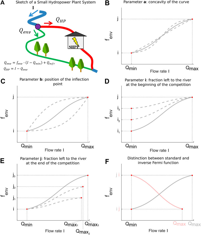
FIGURE 1. (A) Sketch of a run-of-the-river SHP. A part of the natural incoming flow at the intake I (blue line)is diverted to the powerhouse
The flow rate
with
Here, different policies are simulated, the first one being the Minimal Flow Release
with
In order to compare static (i.e., MFR based) and dynamic (e.g., proportional and non-proportional) policies, and to evaluate their performance, a synthetic dimensionless indicator is employed (Razurel et al., 2016, 2018). This ecohydrological indicator is obtained by aggregating the 32 Indicators of Hydrological Alteration (IHA) of Richter et al. (1996), which allows a composite assessment of flow variability (Table 1) and fish habitat suitability. Fish habitat suitability is typically represented by Weighted Usable Area (WUA) curves as modeled with the PHABSIM software (Milhous et al., 1984; Maddock, 1999; Bloesch et al., 2005). Whilst we refer to Razurel et al. (2016) and Razurel et al. (2018) for details, here it suffices to say that Weighted Usable Area (WUA) curves were computed for one dominant fish species, the brown trout, discriminating between juveniles and adults. Although this fish species is not the predominant one in all examined case studies, it better represents common features of the species involved. In particular, we used WUA curves in order to identify the threshold flow rate
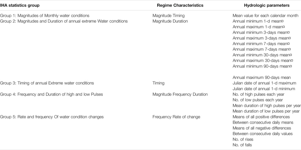
TABLE 1. Summary of hydrological parameters used in the Indicators of Hydrologic Alteration and their characteristics.
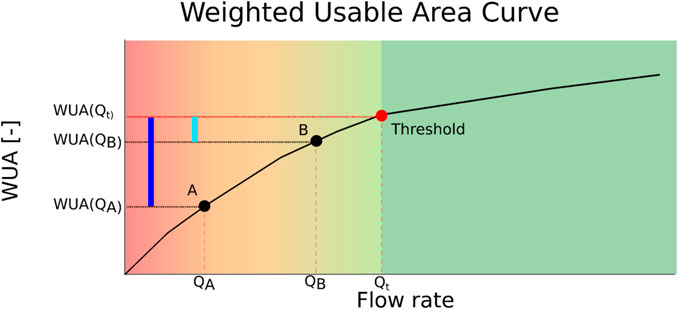
FIGURE 2. Example of a Weighted Usable Area curve modeled with the PHABSIM software (Bloesch et al., 2005; Milhous et al., 1984; Maddock, 1999). The well-being of the fish is shown by the color of the background, green being good and red is bad. It is used to compute the three alternatives of fish habitat suitability indicators
The Indicators of Hydrologic Alteration (IHA) method (Richter et al., 1996), which is based on analysis of hydrological data, defines a set of indicators used to quantify the degree of alteration caused in by the diversion of the water sent to the hydropower plant. As shown in the Table 1, the 32 IHA indicators are sorted into five groups characterizing annual hydrological variations such as magnitude, timing, duration, frequency and rate of change of discharges. In the original stream-scale model (Razurel et al., 2018), all the indicators were given the same weight to compute the final indicator. In this work, we evaluate the influence of each of them on the efficiency plot, i.e., they are all treated separately with no final aggregation.
The economic indicator is defined as the energy production normalized to the maximal production obtained with the
After the environmental and economic indicators are calculated for each water allocation policy scenario, the efficiency plot is built by plotting the energy production
Five run-of-the-river SHP and one traditional hydropower plant (i.e., with storage) subjected to different hydrological regimes, were investigated. Technical details including the turbine nominal flow,
The first goal of the sensitivity analysis is to identify, for each case study, which IHAs produce the efficiency plot with the highest variability, i.e., the IHAs that are the most affected by the distribution policies. To do so, the efficiency plot was computed considering the effect of each hydrological sub-indicator separately. Then, the Pareto frontiers of each of them are compared.
The other parameter used for the computation of the ecohydrological indicator concerns fish habitat suitability. This is used to assess the suitability of the environmental flow regime for selected fish species, i.e., via the WUA curve (Capra et al., 1995). For increasing streamflow magnitude, a break-point appears in the slope of the WUA curve, which is generally assumed as the threshold minimal flow below which habitat conditions for that fish species are critical. In previous studies, this fish ecological indicator,

TABLE 3. Definition of the three alternatives compared in the sensitivity analysis to evaluate the fish habitat suitability indicator (d corresponds to the number of consecutive days under the threshold).
A common problem arising in the analysis of real case studies is the lack of historical data. For the case of Inverliever, for example, only 6 y of hydrological data are available, whereas the IHA method would recommend a minimum of 20 y. To overcome this problem, a 20-y synthetic hydrograph was generated based on the available data series. For this, a back-filtered Periodic Autoregressive Model (PAR) was used (Brockwell et al., 2002). Preliminary transformations to the original series were performed: logarithmic transformation followed by removal of trends and shifts by daily standardization. The model order was then determined using the temporal partial autocorrelation function. After this, the synthetic time series was generated with the AR model, the trend was added back and the series re-transformed. As the synthetically generated time series was still particularly noisy at low-medium flow rates, a moving average filter was applied. In particular, the size of the moving average window was determined with a threshold conserving the water balance and by minimizing the differences for the temporal autocorrelation function and other statistical quantities (minimum flow, maximum flow, mean flow, standard deviation, skewness coefficient) between the observed and generated time series. To validate the model and to compare the generated synthetic hydrograph with the historical data, we also computed the IHAs as non-linear evaluation parameters for both time series. An example of generated synthetic hydrograph is shown in Figure 3.
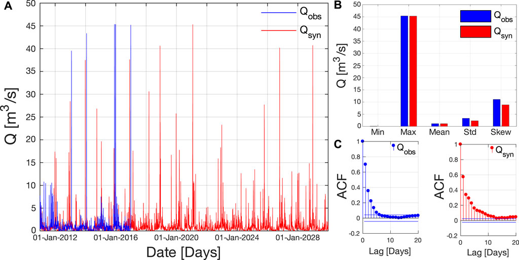
FIGURE 3. (A) Example of synthetic 20-y hydrograph obtained with the back-filtered PAR model based on the 5-y hydrograph for the Inverliever SHP. (B) Comparison of some statistical quantities for the observed and synthetic hydrographs. (C) Comparison of the autocorrelation function of the observed and synthetic hydrographs.
Figure 4 shows the Pareto frontiers obtained when considering each hydrological sub-indicator separately. Colors are used to make the distinction between the different groups. There are five groups in total (Table 1); however, as far as the SHPs are concerned, the third group is not considered in the evaluation because its inclusion would bias the assessment in favor of the release policy. In fact, given the absence of storage, the Julian date of annual 1-d maximum and minimum will be the same for the pre- and post-impact series, so that all policies would have the same impact. For the SHPs we see that most of the Pareto frontiers are almost horizontal and close to unity. This suggests that the IHAs used to assess the location of the Frontier are not affected by the change in water allocation policy. Their values are close to those corresponding to the natural flow regime policy, whence their ineffectiveness for the Frontier. On the other hand, some other IHAs markedly affect the form of the Frontier given that their value is strongly affected by the chosen water redistribution policy.
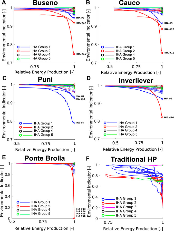
FIGURE 4. Pareto Frontier resulting from non-proportional policies for each of the 32 IHA sub-indicators. Dots represent
IHA 16 affects four out of five SHP case studies (Figures 4A–E). In the original classification of Richter et al. (1996), this indicator corresponds to the highest 3-days value flow rate occurring during the year and is a measure of environmental stress disturbance.
For the five SHP case studies, the Pareto frontiers associated with IHAs of Groups 1 and 2 show more variability than those for Groups 4 and 5. Group 1 includes 12 parameters, each of which measures the mean of the daily water conditions for a given month. It thus provides a general measure of habitat availability or suitability. Group 2 corresponds to the magnitudes and duration of annual extreme water conditions (ranging from daily to seasonal). It also provides measures of environmental stress and disturbance during the year. According to Richter et al. (1996), the Group 2 indicators reflect stress conditions affecting the reproduction of certain fish species.
For the case of the traditional hydropower plant with storage, except for Group 3 indicators, all sub-indicators clearly influence the Pareto Frontier. This means that traditional hydropower plants have a greater ecological impact than SHPs for changing hydrologic regimes, as expected. Hence, while “diverting water” alone is mainly detected by Groups 1 and 2, adding water storage also impacts indicators of Groups 4 and 5.
The next step of the sensitivity analysis is to consider only a few hydrological sub-indicators to re-calculate the Pareto Frontier. That is, only IHAs with the highest impact are considered when computing the environmental indicator. Results are shown in Figure 5 for the power plants of Inverliever, Puni and Ponte Brolla. For the sake of clarity, Buseno and Cauco are not shown as the results are very close to the efficiency plot obtained for Puni. There is a big difference between the red and blue Pareto frontiers, which are, respectively, obtained by considering all IHAs, and only those producing the highest variability (Table 4). This is particularly evident for Puni and Ponte Brolla power plants.
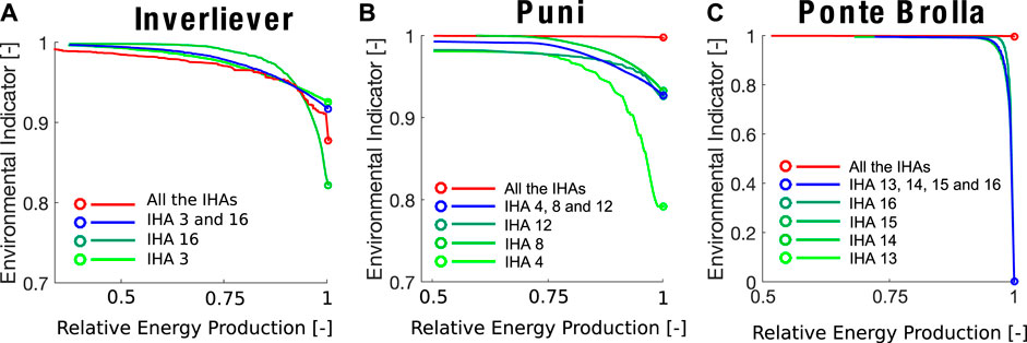
FIGURE 5. Contribution of the IHA with the highest variability identified in Table 4 to compute the new Pareto Frontier (blue curve). The red curve represents the original Pareto Frontier that would be obtained if all the IHAs were taken into account. The dots represent
For Puni and Ponte Brolla, the red Pareto Frontier is almost horizontal, suggesting that assigning equal weight to the hydrological indicators will result in a Pareto Frontier that is independent of the water allocation scenario. Therefore, the weight of the majority of the indicators that are insensitive to flow release policies can blur the effect of the few sensitive ones. However, for Inverliever, the red and blue lines are very close.
Figure 6 shows the efficiency plots for the proportional policies for each of the 32 hydrological sub-indicators. Note that the IHAs determining the highest variability (i.e., the most influential ones for changing water allocation policy) are the same as those in Figure 5. This shows that not only the NPPs are affecting the IHAs but also that the results can be transposed to all the different classes of distribution policies. This leads to the recommendation of performing a preliminary sensitivity analysis in order to identify which sub-indicators should be selected for the sake of meaningfulness of the results.
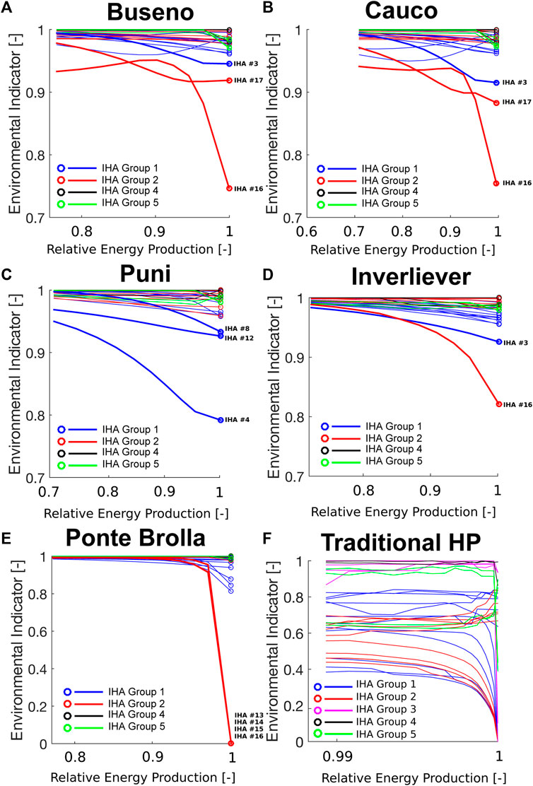
FIGURE 6. Pareto frontiers resulting from improving proportional policies for each of the 32 IHA sub-indicators. Dots represent
Figure 7 shows the Pareto frontiers obtained when considering only the fish habitat suitability indicator to compute the environmental indicator. Each color corresponds to a different choice from Table 3 used to calculate the indicator. For all three cases, the alternative
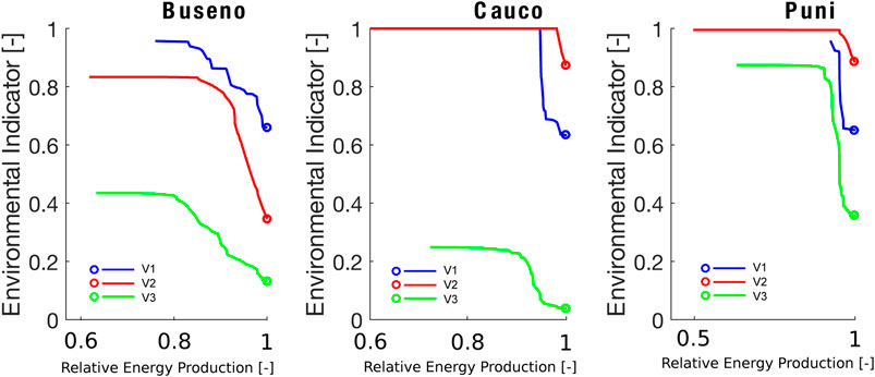
FIGURE 7. Pareto Frontier plots for non-proportional policies for the different versions of the fish indicator
In the IHA method, Richter recommends using a set of at least 20 y of hydrological data to evaluate annual variations of the flow regime. This can be a problem if the river is not monitored or if no gauging station is installed in a nearby catchment. For the Inverliever SHP, only 6 y of data were available so a synthetic 20-y hydrograph was reconstructed using the technique described in Sensitivity analysis, which gives a statistically equivalent flow discharge time series.
For purely ergodic and stationary time series of infinite length, computing the Pareto Frontier starting from different discharge time sequences would reasonably not produce any appreciable change in the resulting Frontier. However, the series have a limited length and the effect of this on the Frontier is not obvious. Hence, 20 alternative hydrograph scenarios were generated and used to estimate the dependency of the Pareto Frontier on the length of the series. The newly generated synthetic hydrographs were found to have almost the same statistical properties as the original, and thus the limited length of the series has a minimal influence on the resulting efficiency plot.
Figure 8 shows the Pareto frontiers resulting from using 20 statistically equivalent discharge sequences obtained from the PAR nonlinearly filtered model. The red line corresponds to the mean Pareto Frontier and the red circle is the average proportional policy with a percentage of 30%. Provided that statistically equivalent hydrograph signals are used, the effect of limited length enhances hydrograph uncertainty. The resulting Pareto frontiers appear therefore distributed around the mean within a band of about 3 percentile points.
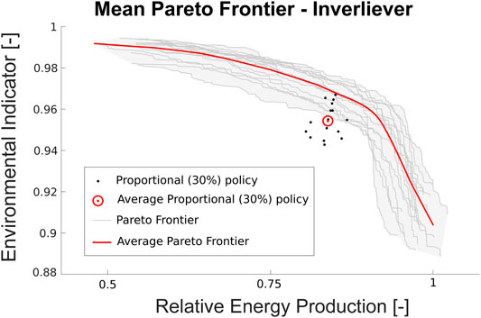
FIGURE 8. Mean Pareto Frontier (red curve) and 30% proportional policy (red dots) resulting from the average of 20 different generations of the 20-y hydrograph for the Inverliever SHP.
In this work we chose to build the efficiency plot by considering the energy production and not the benefit as a key quantity. The advantage of doing this is that this choice will remove any dependency on economic market fluctuations and is more aligned with the unbiased estimate of the actual improvement that could be achieved in view of future energy transition strategies (e.g., the Swiss Energy Strategy 2050). More than for SHP, this can be an issue for traditional hydropower in that storage capacity clearly influences operational decisions. Notwithstanding this, this work provides a quantitative analysis of the global performance of hydropower, which might help identifying the best improvement strategy in view of the future transition towards sustainable energy sources (Willmott et al., 2016). This is also key with respect to the renewal of concession to SHP operating sustainable and globally efficient production policies.
The sensitivity analysis highlights the impact of weighting the IHA indicators to compute the aggregated hydrological indicator. This is more important for computing the performance of SHPs than for traditional hydropower where more or less all indicators have a strong impact on the efficiency plot and can therefore all be weighted equally. Indeed, for the five SHP case studies, most of the IHA indicators (especially from Group 4 and 5) show little or no variation as a function of the water allocation policy. After aggregation, we obtained a horizontal Pareto Frontier very close to the natural regime, which would lead to a misinterpretation of the real performance of the adopted redistribution policy. Group 1 and 2 indicators are more affected by the change in water regime in the case of SHP, and IHA number 16 is common to 4 cases out of 5. A pre-sensitivity analysis would therefore help identify which IHAs are more suitable to represent the impact that the exploitation of a specific stream has on the components of the hydrologic regime.
A limit of the streamflow model used to compute the Pareto Frontier is that each case has to be considered separately and the weighting of the indicators is arbitrary. On the one hand, if one considers only the indicators that are strongly affected by the redistribution rules and removes the others, then the resulting Pareto Frontier will be pessimistically assessed because part of the information of the hydrologic regime variability will not be considered. On the other hand, if equal weight is given to each indicator, then the Pareto Frontier is hardly affected by the redistribution policies, and will result in an optimistic performance with a value very close to unity.
The Fish Habitat Suitability indicator is generally considered important to complement the information from the hydrological indicators and build a comprehensive environmental indicator. The computation of the WUA curve requires river surveys, hydraulic measurements and significant computational power. Fish Habitat Suitability is however biased if used alone because of its dependence on the WUA threshold. This makes it representative of particular ecological species and it should therefore receive a lower weight in most cases unless diversely suggested by other considerations. Moreover, after aggregation, the Fish Habitat Suitability appears to have a stronger influence on the Pareto Frontier than the aggregated hydrological indicator. Each WUA curve is calculated for a specific species and a specific life stage. This would unfairly assess the importance of fish species with respect to other aquatic and terrestrial species that populate the riparian zone and whose adaptation to changing flow regime is better represented by indicators assessing the variability of the hydrological regime.
The differences between the three alternative indicators
Another major issue in assessing hydropower performance is hydrological data availability. While data collection and monitoring are important preliminary tasks for traditional hydropower, the design of SHPs often tolerates qualitatively approximated data. This is because the absence of storage in such plants precludes the need for accurate hydrological and economic forecasts to steer the production policy. However, incomplete data availability hampers evaluation of the long-term global performance of SHPs. Above, we proposed a simple time-series analysis-based model to generate statistically equivalent hydrological time sequences. The comparison of the IHA indicators between the modeled and the measured time series was shown to be a straightforward way to consider nonlinear dependencies in the data structure that would not be taken into account by linear autoregressive models. This modeling approach allowed for computation of the variability of the Pareto Frontier due to the use of short and non-perfectly ergodic time sequences. However, depending on information availability, other streamflow modeling approaches are possible. In particular, where they are feasible we recommend use of physically-based (either spatially distributed or semi-distributed) hydrological models such for example SWAT (https://swat.tamu.edu), or similar.
This study shows that for SHPs, only few among all indicators of hydrological alteration are actually relevant to evaluate the performance of the adopted redistribution rules as far as its hydrological similarities with the natural flow regime are concerned. As a consequence, this simplifies (also computationally) the choice of the best redistribution rule. Moreover, two better alternatives to the currently used fish habitat suitability indicators are also presented. The two different alternatives to the fish habitat suitability indicators proposed by Razurel et al. (2016) improve and strengthen the model by applying a more accurate weighting of the penalty. This construction of the ecohydrological indicator is crucial for evaluation of the efficiency of water distribution rules. Indeed, the sensitivity analysis performed on six different case studies with different water regimes leads to the conclusion that the aggregation method has a strong impact on the assessed environmental performance of the flow release policies. Each indicator evaluates a specific aspect of the impact of the hydropower plant on the environment. Some of them are not relevant in every case as they depend strongly on the characteristics of the river or the type of system (run-of-the-river SHP or traditional dam). Thus, for SHPs, the monthly streamflow magnitude and the magnitude and duration of extreme flow events have the highest influence on the choice of the optimal distribution policies. Conversely, for the traditional hydropower plant with storage, all the IHA groups influence the efficiency plot, including the frequency of high and low pulses and the rate of water condition changes. It is recommended that a preliminary analysis identifying which indicators have to be selected is performed before running the model to find the optimal water allocation rules.
The datasets analyzed and generated for this study can be found in the Zenodo data repository (file:///https://zenodo.org/record/5059557#.YN6beC0RrGY).
PP is the main originator and wrote the article. AN implemented the analyses for the dammed systems. PR implemented the analyses for small hydropower systems. RS implemented the hydrological model, generated the inflow data for the Inverliever power plant. RF, EW, and DB contributed to the structuring phase, read and edited the manuscript.
Authors PP, RF and EW were employed by the company HOLINGER AG.
The remaining authors declares that the research was conducted in the absence of any commercial or financial relationships that could be construed as a potential conflict of interest.
All claims expressed in this article are solely those of the authors and do not necessarily represent those of their affiliated organizations, or those of the publisher, the editors and the reviewers. Any product that may be evaluated in this article, or claim that may be made by its manufacturer, is not guaranteed or endorsed by the publisher.
The authors are grateful to Adrian Loening and Walter Gostner for providing data regarding the SHPs of Inverliever and Puni.
DEF, Dynamic Environmental Flows; FOEN, (Swiss) Federal Office of the ENvironment; HP, Hydropower Plant; IHA, Indicators of Hydrological Alteration; MRF, Minimal Flow Release; PHABSIM, Physical HABitat SIMulation model; PP, Proportional Policies; NPP, Non-Proportional Policies; SEPA, Scottish Environment Protection Agency; SHP, Small Hydropower Plant; WUA, Weighted Usable Area.
Abbasi, T., and Abbasi, S. A. (2011). Small Hydro and the Environmental Implications of its Extensive Utilization. Renew. Sustain. Energ. Rev. 15, 2134–2143. doi:10.1016/j.rser.2010.11.050
Abbasi, T., Premalatha, M., and Abbasi, S. A. (2011). The Return to Renewables: Will it Help in Global Warming Control?. Renew. Sustain. Energ. Rev. 15, 891–894. doi:10.1016/j.rser.2010.09.048
Almeida, R. M., Shi, Q., Gomes-Selman, J. M., Wu, X., Xue, Y., Angarita, H., et al. (2019). Reducing Greenhouse Gas Emissions of Amazon Hydropower with Strategic Dam Planning. Nat. Commun. 10, 4281. doi:10.1038/s41467-019-12179-5
Arthington, A. H., Bunn, S. E., Poff, N. L., and Naiman, R. J. (2006). The challenge of Providing Environmental Flow Rules to Sustain River Ecosystems. Ecol. Appl. 16, 1311–1318. doi:10.1890/1051-0761(2006)016[1311:tcopef]2.0.co;2
Basso, S., and Botter, G. (2012). Streamflow Variability and Optimal Capacity of Run-Of-River Hydropower Plants. Water Resour. Res. 48. doi:10.1029/2012wr012017
Benejam, L., Saura-Mas, S., Bardina, M., Solà, C., Munné, A., and García-Berthou, E. (2016). Ecological Impacts of Small Hydropower Plants on Headwater Stream Fish: From Individual to Community Effects. Ecol. Freshw. Fish. 25, 295–306. doi:10.1111/eff.12210
Bloesch, J., Ortlepp, J., and Ortlepp, J. (2005). An Application of Physical Habitat Modelling to Quantify Ecological Flow for the Rheinau Hydropower Plant, River Rhine. rs 16, 305–328. doi:10.1127/lr/16/2005/305
Brockwell, P. J., Davis, R. A., and Calder, M. V. (2002). Introduction to Time Series and Forecasting, Vol. 2. Springer.
Capra, H., Breil, P., and Souchon, Y. (1995). A New Tool to Interpret Magnitude and Duration of Fish Habitat Variations. Regul. Rivers: Res. Mgmt. 10, 281–289. doi:10.1002/rrr.3450100221
Environment Agency (2013). Environmental Flow Indicator. Tech. Rep. January, Environment Agency. Available at: http://webarchive.nationalarchives.gov.uk/20140328104910/, http://cdn. environmentagency.gov.uk/LIT_7935_811630.pdf/.
Gabbud, C., and Lane, S. N. (2016). Ecosystem Impacts of Alpine Water Intakes for Hydropower: the challenge of Sediment Management. WIREs Water 3, 41–61. doi:10.1002/wat2.1124
Gorla, L., and Perona, P. (2013). On Quantifying Ecologically Sustainable Flow Releases in a Diverted River Reach. J. Hydrol. 489, 98–107. doi:10.1016/j.jhydrol.2013.02.043
Hertwich, E. G., Gibon, T., Bouman, E. A., Arvesen, A., Suh, S., Heath, G. A., et al. (2015). Integrated Life-Cycle Assessment of Electricity-Supply Scenarios Confirms Global Environmental Benefit of Low-Carbon Technologies. Proc. Natl. Acad. Sci. USA 112, 6277–6282. doi:10.1073/pnas.1312753111
Lazzaro, G., Basso, S., Schirmer, M., and Botter, G. (2013). Water Management Strategies for Run-Of-River Power Plants: Profitability and Hydrologic Impact between the Intake and the Outflow. Water Resour. Res. 49, n–a. doi:10.1002/2013wr014210-
Lifshitz, E., and Landau, L. (1984). Statistical Physics (Course of Theoretical Physics, Vol. 5. Oxford: Elsevier
Maddock, I. (1999). The Importance of Physical Habitat Assessment for Evaluating River Health. Freshw. Biol. 41, 373–391. doi:10.1046/j.1365-2427.1999.00437.x
Manzano-Agugliaro, F., Taher, M., Zapata-Sierra, A., Juaidi, A., and Montoya, F. G. (2017). An Overview of Research and Energy Evolution for Small Hydropower in Europe. Renew. Sustain. Energ. Rev. 75, 476–489. doi:10.1016/j.rser.2016.11.013
Marler, R. T., and Arora, J. S. (2004). Survey of Multi-Objective Optimization Methods for Engineering. Struct. Multidisciplinary Optimization 26, 369–395. doi:10.1007/s00158-003-0368-6
Mathews, R., and Richter, B. D. (2007). Application of the Indicators of Hydrologic Alteration Software in Environmental Flow Setting1. JAWRA J. Am. Water Resour. Assoc. 43, 1400–1413. doi:10.1111/j.1752-1688.2007.00099.x
Meijer, K. S., Van der Krogt, W. N. M., and van Beek, E. (2012). A New Approach to Incorporating Environmental Flow Requirements in Water Allocation Modeling. Water Resour. Manage. 26, 1271–1286. doi:10.1007/s11269-011-9958-z
Milhous, R., Wegner, D., Waddle, T., Energy, W., Team, L., Flow, I., et al. (1984). User’s Guide to the Physical Habitat Simulation System (PHABSIM). Department of the Interior, US Fish and Wildlife Service. Available at: http://pubs.er.usgs.gov/publication/fwsobs81_43”/.
Moyle, P. B., and Mount, J. F. (2007). Homogenous Rivers, Homogenous Faunas. Proc. Natl. Acad. Sci. 104, 5711–5712. doi:10.1073/pnas.0701457104
Niayifar, A., Oldroyd, H. J., Lane, S. N., and Perona, P. (2018). Modeling Macroroughness Contribution to Fish Habitat Suitability Curves. Water Resour. Res. 54, 9306–9320. doi:10.1029/2018wr022860
Niayifar, A., and Perona, P. (2017). Dynamic Water Allocation Policies Improve the Global Efficiency of Storage Systems. Adv. Water Resour. 104, 55–64. doi:10.1016/j.advwatres.2017.03.004
Payne, T. R. (2003). “The Concept of Weigthed Usable Area as Relative Suitability index,” in Proceedings of International IFIM Users Workshop (CD), 1–5. Available at: https://www.noaa.gov/sites/default/files/legacy/document/2020/Oct/07354626138.pdf/.
Perona, P., Dürrenmatt, D. J., and Characklis, G. W. (2013). Obtaining Natural-like Flow Releases in Diverted River Reaches from Simple Riparian Benefit Economic Models. J. Environ. Manag. 118, 161–169. doi:10.1016/j.jenvman.2013.01.010
Petts, G. E. (2009). Instream Flow Science for Sustainable River Management. JAWRA J. Am. Water Resour. Assoc. 45, 1071–1086. doi:10.1111/j.1752-1688.2009.00360.x
Poff, N. L., Olden, J. D., Merritt, D. M., and Pepin, D. M. (2007). Homogenization of Regional River Dynamics by Dams and Global Biodiversity Implications. Proc. Natl. Acad. Sci. 104, 5732–5737. doi:10.1073/pnas.0609812104
Poff, N. L., Richter, B. D., Arthington, A. H., Bunn, S. E., Naiman, R. J., Kendy, E., et al. (2010). The Ecological Limits of Hydrologic Alteration (ELOHA): a New Framework for Developing Regional Environmental Flow Standards. Freshw. Biol. 55, 147–170. doi:10.1111/j.1365-2427.2009.02204.x
Razurel, P., Gorla, L., Crouzy, B., and Perona, P. (2016). Non-proportional Repartition Rules Optimize Environmental Flows and Energy Production. Water Resour. Manage. 30, 207–223. doi:10.1007/s11269-015-1156-y
Razurel, P., Gorla, L., Tron, S., Niayifar, A., Crouzy, B., and Perona, P. (2018). Improving the Ecohydrological and Economic Efficiency of Small Hydropower Plants with Water Diversion. Adv. Water Resour. 113, 249–259. doi:10.1016/j.advwatres.2018.01.029
Richter, B. D., Baumgartner, J. V., Powell, J., and Braun, D. P. (1996). A Method for Assessing Hydrologic Alteration within Ecosystems. Conservation Biol. 10, 1163–1174. doi:10.1046/j.1523-1739.1996.10041163.x
Robson, a., Cowx, I. G., and Harvey, J. P. (2011). Impact of Run-Of-River Hydro-Schemes upon Fish Populations. Edinburgh, Scotland: Environment, 1–71. Available at: http://www.sniffer.org.uk/knowledge-hubs/resilient-catchments/water-frameworkdirective-and-uktag-co-ordination/impact-run-river-hydro-schemes-upon-fish-populations/.
Sepa (2014). Guidance for Developers of Run-Of-River Hydropower Schemes. Tech. rep., Scottish Environment Protection Agency. Available at: https://www.sepa.org.uk/media/383805/guidance-_for_developers_of_run_of_river_hydropower_schemes.pdf/.
Keywords: dynamic environmental flows, hydropower, sustainable water management, pareto frontier, water use, non-proportional redistribution, fermi functions
Citation: Perona P, Niayifar A, Schwemmle R, Razurel P, Flury R, Winz E and Barry DA (2021) Frontiers of (Pareto) Optimal and Sustainable Water Management for Hydropower and Ecology. Front. Environ. Sci. 9:703433. doi: 10.3389/fenvs.2021.703433
Received: 30 April 2021; Accepted: 09 July 2021;
Published: 05 August 2021.
Edited by:
Stefano Basso, Helmholtz Centre for Environmental Research (UFZ), GermanyReviewed by:
Alban Kuriqi, Universidade de Lisboa, PortugalCopyright © 2021 Perona, Niayifar, Schwemmle, Razurel, Flury, Winz and Barry. This is an open-access article distributed under the terms of the Creative Commons Attribution License (CC BY). The use, distribution or reproduction in other forums is permitted, provided the original author(s) and the copyright owner(s) are credited and that the original publication in this journal is cited, in accordance with accepted academic practice. No use, distribution or reproduction is permitted which does not comply with these terms.
*Correspondence: Paolo Perona, cGFvbG8ucGVyb25hQGVwZmwuY2g=
Disclaimer: All claims expressed in this article are solely those of the authors and do not necessarily represent those of their affiliated organizations, or those of the publisher, the editors and the reviewers. Any product that may be evaluated in this article or claim that may be made by its manufacturer is not guaranteed or endorsed by the publisher.
Research integrity at Frontiers

Learn more about the work of our research integrity team to safeguard the quality of each article we publish.