Construction of the Mean Sea Surface Model Combined HY-2A With DTU18 MSS in the Antarctic Ocean

A new Mean Sea Surface (MSS) model called Shandong University of Science and Technology Antarctic Mean Sea Surface model (SDUST_ANT MSS) in the Antarctic Ocean is presented and validated in this paper. The SDUST_ANT MSS updates the DTU18 MSS with 6 years of Exact Repeat Mission (ERM) and Geodetic Mission (GM) data from HY-2A. Collinear adjustment was applied to all the ERM data to obtain the along-track mean sea surface height. Oceanic variability has been removed from the GM data. Crossover adjustment was applied to both the ERM and GM data. We constructed the HY-2A_MSS using HY-2A altimetry data based on optimal interpolation method. Several types of errors (such as white noise, residual effect of oceanic variability, and long wavelength bias) have been taken into account for the determination of MSS using optimal interpolation method. The SDUST_ANT MSS was constructed by mapping HY-2A_MSS onto the DTU18 MSS. The SDUST_ANT MSS was compared with DTU18 MSS and CNES_CLS15 MSS. At wavelengths below 150 km, differences between models are consistent with seafloor topographic gradient. At wavelengths above 150 km, differences are affected by the mesoscale activities and the altimetry errors in coastal areas. The errors of the three models, as indicated by their power spectral densities (PSDs), are of similar orders of magnitude. The absolute error is slightly smaller in SDUST_ANT than in CNES_CLS15 or DTU18.

Introduction

The Mean Sea Surface (MSS) is an essential parameter in oceanography and geophysics. Geodetic and hydrographic surveys adopt the MSS or a reference surface that is related to the MSS as their datum. An accurate MSS is necessary for the analysis of oceanic variability using satellite altimetry and can be used for the calibration or validation of satellite altimetry data (Jin et al., 2016). Oceanic variabilities are dominated by seasonal variability and interannual signal, they also include sea surface anomalies caused by large scale oceanographic anomalies (such as El Nino and La Nina) occurring at specific times.

The emergence of satellite altimetry technology has changed the way that we understand and observe the Earth, especially the oceans. Substantial improvements in the spatial and temporal resolution of altimetry data have ushered global ocean system research into a new era. The satellite Skylab carried the first altimeter into space in 1973. Satellite altimetry was initially used for telemetry and has since been used to determine the structure of the sea surface and applied widely across the fields of geophysics and geodesy. Because satellite altimetry technology can repeatedly provide accurate information on the surface height of oceans throughout the world, it provides a wealth of data for studies of sea level change, the gravitational field, seafloor topography, marine lithosphere, and ocean circulation.

Since 1991, the radar altimeters onboard the European Space Agency (ESA) satellites ERS-1/2 and Envisat have been collecting data over the Southern Ocean and also over the sub-polar seas between 81.5°N and 81.5°S. In recent decades, satellite altimetry coverage has extended further towards the poles through dedicated polar missions. For example, NASA’s ICESat (2003–2010) reached up to ±86 in latitude; ESA’s CryoSat-2 (2010–present) reaches up to ±88 in latitude (Peacock and Laxon, 2004); NASA’s ICESat-2 mission reaches ±88 in latitude and provides nearly complete coverage of the polar region. The ICESat-2 mission carries the Advanced Terrain Laser Altimeter System (ATLAS), which was launched at the end of 2018. Complementary measurements are provided by the SARAL/AltiKa (2013–present) and Sentinel-3 (2016–present) (Skourup et al., 2017).

Existing MSS models of the Antarctic Ocean are based on data from some of the altimetry missions; these models include the ERS-2 MSS (Peacock and Laxon, 2004), the ICESat–Envisat (ICEN) MSS (Farrell et al., 2012), and a CryoSat-2 MSS developed at University College London (Au Ridout, 2014). The Danish Technical University (DTU) has developed several global MSS models that cover the Antarctic Ocean; these models include the DNSC08 MSS, DTU10 MSS, DTU13 MSS, DTU15 MSS, and DTU18 MSS and use different combinations of data from ERS-1/2, Envisat, ICESat, and CryoSat-2 (Andersen and Knudsen, 2009, 2011; Andersen et al., 2010; Andersen et al., 2015; Andersen et al., 2016; Andersen et al., 2018a; Andersen et al., 2018b). The CNES_CLS global MSS models, which include the CNES_CLS11, CNES_CLS15, and CNES_CLS19 (Schaeffer et al., 2012; Schaeffer et al., 2017; Pujol et al., 2020). The WHU2000 MSS, WHU2009 MSS, and WHU2013 MSS models developed at Wuhan University in China (Jiang et al., 2002; Jin et al., 2011; Jin et al., 2016) also comprise data from multiple altimetry missions.

Spatial coverage and resolution, reference periods, and satellite altimeters for the most recent DNSC08, DTU, CNE_CLS, and WHU MSS models are summarized in Table 1, except for the CNES_CLS19 MSS, which has not yet been released.

TABLE 1

TABLE 1. Overview of recent MSS models.

The aim of this paper is to investigate a method to merge new altimetry data into conventional mean sea surface models in order to derive the next generation MSS. In this research, we show the case study of merging the Chinese HY-2A altimetry data to the present DTU18 MSS model over Antarctic ocean. It is extremely difficult to obtain information about the sea surface at high latitudes. Proximity to the poles, presence of sea ice, the strong ocean currents around the Antarctic, and the paucity of satellites have resulted in reduced quality and temporal and spatial coverage of satellite altimetry data from the high latitudes (Andersen and Knudsen, 2009). So the Antarctic ocean is the good choice to test our method. China’s first satellite for the measurement of ocean dynamic and environmental parameters, such as sea surface wind field, sea surface height, significant wave height and sea surface temperature, etc. HY-2A, has been in orbit for more than 6 years and has collected a large amount of data on its Exact Repeat Mission (ERM) (2 years) and Geodetic Mission (GM) (4 years). These data will complement existing data from other sources, provide valuable information for the study of the MSS and oceanic mesoscale activities and have not yet been included in any MSS model. This paper describes the development of the Shandong University of Science and Technology Antarctic (SDUST_ANT) MSS model on the basis of the earlier DTU18 MSS model and HY-2A altimetry data.

Data and Models

Altimetry Data

HY-2A Data

The satellite HY-2A was launched on 16 August 2011, and the data were released by China’s National Satellite Ocean Application Service (NSOAS). The projected orbital inclination of HY-2A is 99.34, providing a revisit time of approximately 14 days and different orientations of ground tracks during the first part of the operational life of the satellite (Zhao and Zhou, 2013). On GM phase (approximately 168 days) during the second part of its operational life, HY-2A entered into drift orbit, which increased the spatial coverage of the altimeter (Zhang et al., 2018).

The data used here are the along-track Level-2 Plus (L2P) products released by Archiving Validation and Interpretation of Satellite Oceanographic Data (AVISO). The 1 Hz HY-2A data have been adjusted to have the same reference ellipsoid and frame as TOPEX/Poseidon (T/P) data and have been corrected for instrumental errors, sea state bias, tidal effect, and atmospheric pressure.

Instrumental errors are mainly due to internal delays of the instrument, but can also be caused by attitude errors. The sea state bias is an altimeter ranging error due to the presence of ocean waves on the surface (Passaro et al., 2018). Tidal effect includes the effect brought from ocean tide, ocean tide loading, solid Earth tide, and pole tide. Ocean tide is the perturbation of the ocean free surface elevation relative to the seabed. Solid Earth tide is due to the direct attraction of the Sun and Moon on the deformable solid Earth. Ocean tide loading is the deflection of the deformable seabed by the tide-induced anomalous weight of water above it. Pole tide is the ocean response to the variation of both the solid Earth and the oceans to the centrifugal potential that is generated by small perturbations to the Earth’s rotation axis. Atmospheric pressure, also known as barometric pressure (after the barometer), is the pressure within the atmosphere of the Earth.

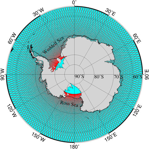
The details of the instrumental and geophysical corrections are given in the L2P product handbook. We used the 2-year ERM data from April 2014 to March 2016 (cycle 067–117) as well as the 4-year GM data from March 2016 to March 2020 (cycle 118–281). The ground tracks of HY-2A ERM are shown in Figure 1 and special areas are marked in Figure 1.

FIGURE 1

FIGURE 1. Geographical distribution of a typical HY-2A 14-day near-repeat altimetry ground tracks.

Evaluation of HY-2A Satellite Altimetry Data in the Antarctic Ocean

To assess the HY-2A satellite altimetry data in the Antarctic Ocean, we compared the distribution of SSH from SARAL/AltiKa, CryoSat-2, and HY-2A satellite altimetry data for the period between 20141206 and 20141220 (cycle 84 of HY-2A) and the period between 20140607 and 20140621 (cycle 71 of HY-2A) (Cheng and Andersen, 2014). Figures 2, 3 show that there is high consistency between the datasets. SSH is the lowest in the Ross Sea and the highest in the Indian Ocean. In the areas covered by sea ice, data quantity and spatial coverage are higher in summer than in winter and the quantity of observations is lower over the Ross Sea and the Weddell Sea than in other parts of the study area. Table 2 shows that the standard deviation (STD) of the mono-mission crossover differences (SSH differences in the crossovers of descending and ascending orbits) is higher in winter than in summer. STD of the HY-2A data is higher than that of the SARAL/AltiKa data and lower than that of the CryoSat-2 data. Among the three datasets and for the same data acquisition period, data quantity is the highest for HY-2A. Combining the three datasets, data quantity is higher in summer than in winter. On the basis of our analysis of SSH values and crossover differences, we conclude that there is high consistency between the datasets, which confirms the good performance of the HY-2A altimeter. Moreover, it is possible to extend the sea level time series by combining HY-2A satellite altimetry data with other satellite altimetry datasets or MSS models for the construction of a new MSS model and the studying of sea level change and climate change.

FIGURE 2

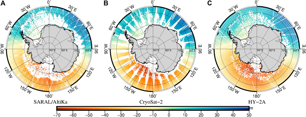
FIGURE 2. The distribution of sea surface height observed from (A) SARAL/AltiKa, (B) CryoSat-2, and (C) HY-2A satellite altimetry for the same period between 20141206 and 20141220.

FIGURE 3

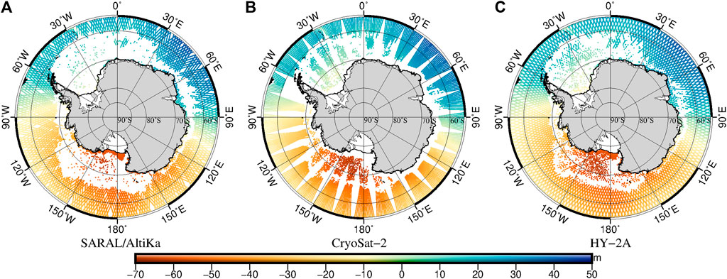
FIGURE 3. The distribution of sea surface height observed from (A) SARAL/AltiKa, (B) CryoSat-2, and (C) HY-2A satellite altimetry for the same period between 20140607 and 20140621.

TABLE 2

TABLE 2. Comparisons of SARAL/AltiKa, CryoSat-2, and HY-2A satellite altimetry data.

Sentinel-3A Data

Sentinel-3A mission was launched on 16 February 2016 by ESA to an orbit of altitude 814 km. The satellite caries one altimeter radar called SRAL (SAR Radar ALtimeter), a dual-frequency SAR altimeter (Ku-band at 13.575 GHz and C-band at 5.41 GHz). 20 Hz data from Sentinel-3A was used to evaluate and validate the MSS errors. The Sentinel-3A altimeter operates in Synthetic Aperture Radar Mode, with an along-track spatial resolution of 300 m in this mode, and provides useful observations of sea level in coastal areas (EUMETSAT, 2018). The data was downloaded from Copernicus Online Data Access. Cycles 54 and 63 were selected to estimate the MSS errors.

The DTU18 Mean Sea Surface Model

The DTU18 MSS is the newest version of the global high resolution MSS released from DTU Space. The new major advance leading up to the release of DTU18 MSS is the use of the Sentinel-3A record for 3 years and an improved CryoSat-2 Low Resolution Mode record for 7 years. A new processing chain with updated editing and data correction (i.e., using FES2014 as the ocean tide model) has been implemented. The use of a consistent ocean tide model for the mean sea surface and the subsequent processing of sun-synchronous satellites have reduced the contribution of the MSS to the total error budget (Andersen, et al., 2018a). Four steps to update the DTU18 MSS. I) Retracking and reprocessing of CryoSat-2 within leads. II) Long wavelength correction TP/J1/J2 mean profiles. III) Coastal zone update using Sentinel-3A and TP/J1/J2 + TDM (Tandem Phase) profiles. IV) Removing geodetic mission oceanic variability in interpolation (Andersen, et al., 2018a; Andersen, et al., 2018b).

Methods

In general, MSS models are constructed following these steps: data selection and preprocessing, unification of temporal and spatial references, collinear adjustment of ERM data, removal of the temporal oceanic variability from GM data, crossover adjustment, and gridding. The gridded product is combined with DTU18 MSS to construct new generation MSS.

Collinear Adjustment of HY-2A Exact Repeat Mission Data

Collinear adjustment is an effective method to reduce the time-varying effect of sea level based on the characteristics of repeated orbit design of altimetry satellites. Ground trajectories of altimetry satellites with ERM do not coincide, the 14-day Exact Repeat Orbit retraces the HY-2A ERM ground track within ±1 km. Therefore, we calculated the average trajectory and average sea level from repeat orbit altimetry data to reduce the influence of the variability of sea level with time, and especially the effects of abnormal sea level changes caused by large-scale oceanographic anomalies on the results.

The average trajectory was obtained by calculating the average between the reference and the collinear trajectories. The trajectory with stable and well-observed data in the repeated period observation data participating in the collinear was selected as the reference trajectory, and the other repetitive period observation data were interpolated into the reference trajectory. At each point along the reference trajectory, SSH was obtained using the collinear method; the difference between sea level on the reference trajectory and sea level on the collinear trajectory was calculated, and the data point was removed from the collinear trajectory if the difference exceeded 0.5 m. To ensure that annual variations in sea level are absent in the adjusted data, cycles that are shorter than one year were excluded from the collinear adjustment (Jin et al., 2011).

Oceanic Variability Correction of HY-2A Geodetic Mission Data

Removing oceanic temporal variability from the GM data was the main challenge that we encountered in the processing of HY-2A data for the MSS model. Because of the limited revisit time of the GM data, the influence of oceanic variability cannot be eliminated or reduced by averaging over multi-year data. Instead, it can be solved by daily, monthly, seasonal, and annual sea level anomaly (SLA) models that are based on simultaneous satellite data. We corrected interannual and seasonal oceanic variability of the GM data using daily gridded SLA maps provided by AVISO/Copernicus (http://marine.copernicus.eu/) (Andersen et al., 2018a; Andersen et al., 2018b). Daily gridded SLA maps were estimated from all altimeter missions using three-dimensional optimal interpolation, which was designed to generate regular gridded SLA products by combining the measurements of various altimeters (Le Traon and Ogor., 1998b, 2003; Ducet et al., 2000; Tierney et al., 2000; Taburet et al., 2019). The reference datum of the corrected grid SLA maps is the same as the datum of the HY-2A GM data, which is the MSS_CLS_15. The corrected SSH was derived as follows (Schaeffer et al., 2012):

$SS{H}_{cor}\left(t,\lambda ,\phi \right)=SSH\left(t,\lambda ,\phi \right)-\left[SL{A}_{\left(t,\lambda ,\phi \right)}^i\right](1)$

$SS{H}_{cor}\left(t,\lambda ,\phi \right)$represents the corrected $SSH\left(t,\lambda ,\phi \right)$ of the satellite minus the results of the Optimal Analysis of a set of SLAs calculated from all satellites. $\left[SL{A}_{\left(t,\lambda ,\phi \right)}^i\right]$ is the interpolated value that would be corrected for oceanic variability at the spatial and temporal position.

Crossover Adjustment

Crossover adjustment is a method generally used to combine multi-mission altimetry data, including ERM and GM data, and to reduce orbit errors, residual oceanic variability, and various physical correction errors. It can weaken the long-wavelength variations of sea level, but the residual radial orbit error, the short-wavelength signal of sea surface variations, and the residual geophysical correction also influence the MSS. At the crossover point between the ascending and descending arcs, the sea level measured on the ascending arc differs from that measured on the descending arc because of the influence of the residual radial orbit error and other factors. Crossover adjustment is one of the main methods to weaken the influence of satellite radial orbit errors and other factors on altimetry data.

Crossover adjustment is used to integrate different satellite altimetry data (including ERM and GM data) or to determine the corrections that need to be applied to measurements on the basis of the difference between two observations from the same location (Huang et al., 1999; Huang et al., 2008). The classical crossover adjustment considers the radial orbit error to be one of the main sources of error affecting altimetry data and that error can be fully modeled by using either a time- or a distance-dependent polynomial (Wagner, 1985; Rummel, 1993). The classical crossover adjustment was modified and simplified by Huang et al. (Huang et al., 1999; Huang et al., 2008; Yuan et al., 2020a; Yuan et al., 2020b). Condition adjustment was applied to the crossover observation equation, and the new error model was used for least squares filtering and estimation along the satellite track. The calculation process did not involve rank deficiency and is suitable for global intersection adjustment.

Construction of HY_2A_Mean Sea Surface Using Optimal Interpolation

The HY-2A_MSS has been computed using the Optimal Interpolation method. The method is based on an optimal interpolation (Le Traon and Ogor, 1998b; Schaeffer et al., 2012):

${\theta }_{est}\left(\stackrel{\rightharpoonup }{x}\right)={\displaystyle \sum _{i=1}^N{\displaystyle \sum _{j=1}^N{A}_{ij}^{-1}{C}_{xj}{\Phi }_{obs,j}}},(2)$

where ${\theta }_{est}\left(\stackrel{\rightharpoonup }{x}\right)$ is the estimated MSS height at the grid point x, ${\Phi }_{obs,j}$ is satellite observation at j, $C_{xj}$ is the covariance/correlation function between satellite observation at j and data at x, $A_{ij}^{-1}$ is the covariance matrix between observations and their noise budget C(r,t), which is given by:

$C\left(r,t\right)=\left[1+ar+1/6{\left(ar\right)}^2-1/6{\left(ar\right)}^3\right]\exp \left(-ar\right)\exp \left(-t^2/T^2\right),(3)$

where $r$ is the distance between two altimetry observations. $a=3.34/L$, $L$ is the space correlation radius, $L$is usually 100∼200 km, here is 150 km (Le Traon et al., 1998a). $t$ is time, and $T$is the temporal correlation radius.

Various types of errors that determine the behavior of the optimal interpolation and the covariance model were taken into account. To determine the new MSS model, we calculated the error budget of altimetric heights by considering the following terms (Schaeffer et al., 2012):

• a noise budget (relating to the instrumental noise), which was expressed as white measurement noise. A white measurement noise of 3 cm was used for HY-2A data. Further details are given in Copernicus Marine Environment Monitoring Service–Sea Level Thematic Assembly Center Product User Manual (CMEMS, 2018);

• the error caused by the residual effect of the oceanic variability, which was to prescribe a spatially correlated error (at the mesoscale wavelength) without affecting the shorter wavelengths of the geophysical static field (Wessel and Smith, 1995);

• following the method proposed by Le Traon and Ogor (1998b), along-track biases are considered. By introducing this term, it is possible to reduce many of these biases caused by along-track errors. This means a better correction of residual errors, for example, geographical correlated orbit errors and imperfections of environmental corrections that may affect missions differently. This aspect is implemented when the wavelength is greater than 100 km and greatly reduces the tracking effect of the MSS grid.

Combination Method

The SDUST_ANT MSS is obtained through a two-step procedure. The HY-2A_MSS was initially mapped from the ERM and GM data using the optimal interpolation method. Then the HY-2A_MSS was subsequently used the remove-restore method to map the SDUST_ANT MSS from DTU18 MSS (Andersen and Knudsen, 2011; Schaeffer et al., 2012; Andersen et al., 2018b). The DTU18 MSS was removed from the HY-2A_MSS to obtain the remaining SSH. The remaining SSH was computed using a spherical harmonic expansion. Then the SDUST_ANT MSS was achieved through the restoration of the DTU18 MSS.

Results and Validation

The Results of Shandong University of Science and Technology Antarctic Mean Sea Surface

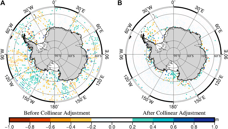
Collinear adjustment was applied to the ERM data. Before collinear adjustment, the STD of crossover differences is 19.82 cm; after adjustment, the STD is 13.81 cm. After adjustment, the accuracy of the ERM data is higher, and the influence of oceanic variability on the data is reduced.

Figure 4 shows what can be achieved by collinear adjustment. Figure 4A shows crossover differences before the collinear adjustment and Figure 4B shows crossover differences after collinear adjustment. In the open ocean, especially in the Pacific Ocean, crossover differences are considerably larger after adjustment. In the offshore sea area, especially in the Weddell Sea and the Ross Sea, crossover differences remain large after adjustment.

FIGURE 4

FIGURE 4. Crossover differences before (A) and after (B) collinear adjustment.

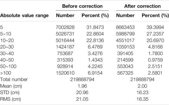
The GM data were addressed by oceanic variability corrections and the results of crossover differences before and after the correction listed in Table 3, which shows that the effect of the oceanic variability on the GM data has been reduced and the accuracy of the SSH has been significantly improved. There are also fewer grid points with a crossover difference above 10 cm, and points with a crossover difference below 10 cm make up a larger proportion of the total number of grid points. The Root Mean Square (RMS) of the crossover differences is 21.05 cm before oceanic variability correction and is 16.35 cm after correction. The improvement is significant after oceanic variability correction.

TABLE 3

TABLE 3. Statistics of the crossover differences before and after correction of GM observations.

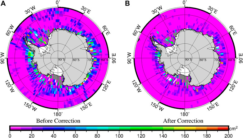
Figure 5 shows the effects of oceanic variability correction. It shows the variance of the SLA signal along HY-2A tracks, before and after removing the oceanic variability (Figures 5A,B, respectively). Variance of SLA before correction shows mesoscale variability; it is dominant in the circumpolar current and the coastal areas and can exceed 400 cm². Oceanic variability correction is more effective in the open ocean and less effective in coastal sea areas. The correction has removed the bulk of the energy, although residual variability remains. Oceanic variability at wavelengths below 200 km (Copernicus Marine Environment Monitoring Service (CMEMS), 2018; Pujol et al., 2018; Taburet et al., 2019) cannot be accurately eliminated by the correction procedure because of limits imposed by the resolution of the daily gridded SLA maps.

FIGURE 5

FIGURE 5. The variance of HY-2A SLA before (A) and after (B) oceanic variability correction.

The results of statistical analyses of the crossover differences of HY-2A altimetry data before and after crossover adjustment are shown in Table 4. It can be seen from Table 4, the RMS of crossover differences have decreased after crossover adjustment both ERM and GM data.

TABLE 4

TABLE 4. Statistical results of crossover differences of HY-2A data before and after crossover adjustment.

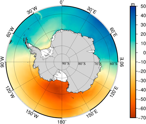
The SDUST_ANT MSS is obtained through the combination method and shown in Figure 6.

FIGURE 6

FIGURE 6. SDUST_ANT MSS in the antarctic ocean.

Evaluation and Validation

The accuracy of MSS models is usually verified via comparisons with other models and mean along-track altimetry observations (Andersen and Knudsen, 2009). In principle, the difference between various MSS models is determined by several factors: the dataset used in the model, the data processing method, and the gridding method. The SDUST_ANT MSS was compared and validated with the DTU18 MSS and the CNES_CLS15 MSS, which are the most widely used global MSS models.

Inter-model Comparison

In evaluating the SDUST_ANT MSS, it is worth examining the differences between SDUST_ANT MSS, DTU18 MSS and CNES_CLS15 MSS Outliers of the difference are rejected by three times STD to avoid contamination by poor observations around coastal areas and islands. The results are listed in Table 5. The difference between the SDUST_ANT MSS and the DTU18 MSS is smaller than the difference between the SDUST_ANT MSS and the CNES_CLS15 MSS.

TABLE 5

TABLE 5. Comparisons of different MSS models.

The largest differences between SDUST_ANT MSS and DTU18 MSS are located in the Weddell Sea and in coastal areas (Figure 7A). The largest differences between SDUST_ANT MSS and CNES_CLS15 MSS are located in the Pacific Ocean–Southern Ocean, Atlantic Ocean–Southern Ocean, and in coastal areas where sea ice is present (Figure 7B).

FIGURE 7

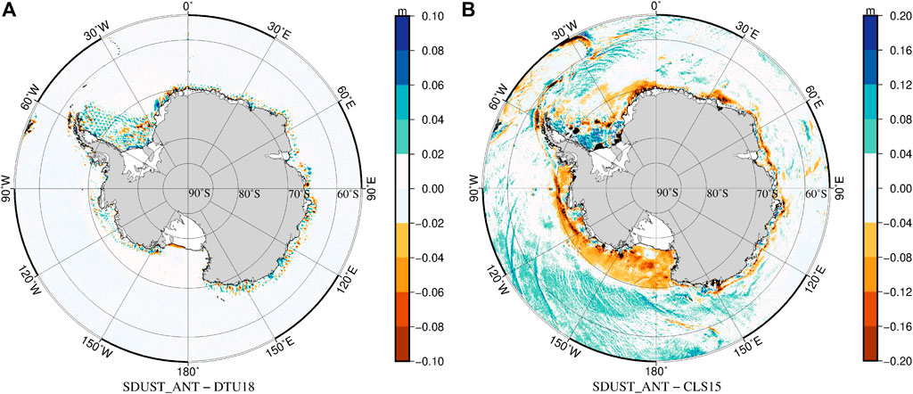
FIGURE 7. (A) Differences between SDUST_ANT MSS and DTU18 MSS and (B) differences between SDUST_ANT MSS and CNES_CLS15 MSS in the Antarctic Ocean after deleting 3 times’ STD error.

A Gaussian filtered solution of the difference between the SDUST_ANT MSS and DTU18 MSS and between the SDUST_ANT MSS and CNES_CLS15 MSS in the Antarctic Ocean was adopted to compare the difference at different wavelengths. We used the tools available in the software Generic Mapping Tools (Wessel and Smith, 1995; Wessel and Smith, 1998) and calculated the differences between the models using a high-pass and low-pass Gaussian filter at the wavelength of 150 km. Figure 8 shows the difference between the SDUST_ANT MSS and DTU18 MSS and the difference between the SDUST_ANT MSS and CNES_CLS15 MSS at short wavelengths (<150 km); the seafloor topographic gradient was calculated from the GEBCO_2020 Grid. At short wavelengths, there is no significant difference between SDUST_ANT MSS and DTU18 MSS (Figure 8A), while there are some differences between SDUST_ANT MSS and CNES_CLS15 MSS (Figure 8B), which can be mainly attributed to differences between DTU18 MSS and CNES_CLS15 MSS. Differences between SDUST_ANT MSS and CNES_CLS15 MSS or between DTU18 MSS and CNES_CLS15 MSS are related to seafloor topographic structures at medium and short wavelengths. The horizontal gradients of the geoid and the MSS are related to the seafloor topographic gradient (Rapp and Yi, 1997; Jimenez-Munt et al., 2008; Sandwell et al., 2014). Examination of Figures 8B,C reveals some correlation between MSS differences and the topographic gradient. Pearson correlation coefficient is 0.2269. Where the absolute value of the gradient is large, the MSS differences are also relatively large; this can be seen near 30°W (along the East Scotia Ridge, the South Sandwich Trench, the South Sandwich Fracture Zone, and the North Weddell Ridge), near 120°W (the Heezen Fracture zone, the Tharp Fracture zone, the Udintsev Fracture zone, and the Pacific–Antarctic Ridge), on the Kerguelen Plateau near 75°E, and in West Antarctica. These special topographic features are marked in Figure 8D.

FIGURE 8

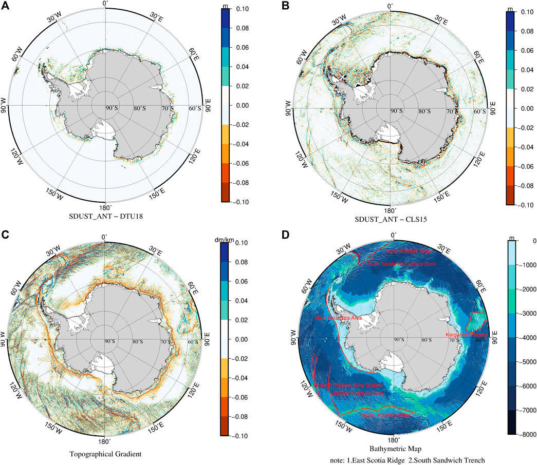
FIGURE 8. Differences at the wavelength shorter than 150 km between SDUST_ANT MSS and DTU18 MSS (A) and differences between SDUST_ANT MSS and CNES_CLS15 MSS (B) in the Antarctic Ocean. (C) Topographical gradient calculated from GEBCO. (D) GEBCO Bathymetric Map with special topography.

At the long wavelengths (>150 km), the difference between SDUST_ANT and DTU18 (Figure 9A) is smaller than the difference between SDUST_ANT and CNES_CLS15 (Figure 9B), which still contains residuals of oceanic variability. In coastal areas, the oceanic variability in the HY-2A data has not been completely removed. The SDUST_ANT differs more from CNES_CLS15 than from DTU18 possibly because of differences in the satellite data that are included in the models and in data processing methods. Between 55°S and 60°S, the differences between SDUST_ANT and CNES_CLS15 are consistent with the spatial distribution of mesoscale activities in the Southern Ocean Antarctic Circulation (Duan et al., 2016; Cui et al., 2020).

FIGURE 9

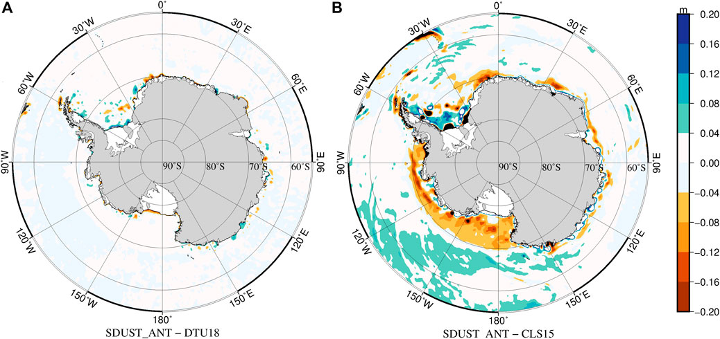
FIGURE 9. (A) Differences between SDUST_ANT MSS and DTU18 MSS and (B) differences between SDUST_ANT MSS and CNES_CLS15 MSS in the Antarctic Ocean at the wavelength longer than 150 km.

Comparison Along Sentinel-3A Tracks Using Power Spectral Density

A sophisticated method is used to derive the absolute error of each model. The methodology is detailed in Pujol et al. (2018). The sum and difference of the SLAs from two cycles can be used to infer the absolute MSS error if the cycles are selected to minimize the oceanic variability correlation. Sentinel-3A described in Sentinel-3A Data Section 2.1.3 was used to calculate the absolute MSS error spectrum.

Essentially, by using the difference between SLAs of the same tracks separated by several months, the true SLA PSD can be inferred, because both SLAs are decorrelated and the MSS errors cancel one another out. So it is possible to obtain the PSD of the absolute MSS error.

The thin colored lines in Figure 10 show the PSD of the measured SLA (i.e., including the MSS error) using the three MSS models. Using the difference between the SLAs of two cycles separated by 269 days, we can deduce the thin black line which is the true PSD of the SLA signal with the instrumental noise (no more MSS error). The MSS error is stationary and has been canceled out prior to the computation of the PSD and is therefore excluded from the values indicated by the black line in Figure 10.

FIGURE 10

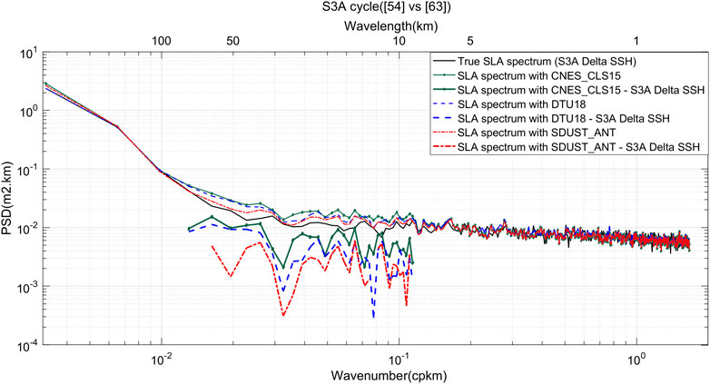
FIGURE 10. PSD of the true SLA signal with instrumental noise (thin black line), SLA signal including the MSS error (thin color lines), MSS errors (thick color lines) with statistically significant (95% confidence threshold). SLA computed using CNES_CLS15 (green), DTU18 (bule), SDUST_ANT (red).

The PSD of the MSS error for the three MSS models (thick colored lines in Figure 10) were calculated from the difference between the PSD of the measured SLA using the models (thin colored lines in Figure 10) and the true PSD of the SLA signal (thin black line in Figure 10). Our results are only valid for small wavelengths where the difference between two PSDs is significant (usually between approximately 8–10 km and 80–100 km). The error is the largest in the CNES_CLS15 and is the smallest in the SDUST_ANT. Figure 10 shows that the green PSD of CNES_CS15 is 2 times larger than the red PSD of the SDUST_ANT model. The blue PSD of DTU18 is 1.5 times larger than the red PSD of the SDUST_ANT model.

Discussions

This paper compared the altimetry data of HY-2A with the altimetry data of SARAL/AltiKa and with that of CryoSat-2 in the Antarctic Ocean and found consistency between the three datasets.

HY-2A satellite altimetry observations and DTU18 MSS were combined to establish an Antarctic MSS model named SDUST_ANT, using the mean along-track SSH of HY-2A satellite series observations spanning 2-year between 2014 and 2016 after collinear adjustment and the GM SSH spanning 4-year between 2016 and 2020 after the correction the oceanic variability.

We used the mean along-track SSH of T/P satellite series observations between 1993 and 2012 with collinear adjustment as the reference datum. Collinear adjustment was used to correct or eliminate the oceanic variability of the HY-2A ERM observations, while the daily gridded SLA maps were used to correct HY-2A GM observations. The influence of residual oceanic temporal variability and radial orbit error was eliminated by crossover adjustment. The HY-2A_MSS was computed using optimal interpolation. Using DTU18 MSS as the reference field, the SDUST_ANT MSS was created following the remove–restore method.

We calculated the differences between DTU18 MSS, CNES_CLS15 MSS, and SDUST_ANT MSS, and found that at short wavelengths (<150 km), differences between the models are consistent with the topography structure. It’s shown by Pearson’s correlation coefficient, there is a weak linear correlation between differences and the topographic structure. But as can be seen from Figure 8, it has strong correlation with the seabed topographic structure. Therefore, the nonlinear correlation between the difference at short wavelengths (<150 km) and the topographic structure needs to be further explored. At long wavelengths (>150 km), mesoscale activities are the dominant source of MSS error in the open ocean, while altimetry error (due to range and geophysical corrections) is the dominant source of error in coastal areas. We estimated the absolute error of SDUST_ANT MSS along the Sentinel-3A tracks and focused on the mesoscale. The absolute error of SDUST_ANT is slightly smaller than that of the CNES_CLS15 and that of DTU18. Therefore, under the premise of determining the temporal and spatial scales of the combined satellite altimetry data, it is feasible to integrate the data with the MSS model to improve the former MSS model.

Conclusion

In conclusion, the comparison results between HY-2A, SARAL, and CryoSat-2 are consistent with each other. It is possible to extend the sea level time series by combining HY-2A altimetry data with other satellite altimetry data for mean sea surface model and for climate change research.

The process of the establishment of the MSS also have been presented, including collinear adjustment of ERM data, removal of the oceanic variability from GM data, crossover adjustment and gridding. The gridding map is combined with the DTU18. After validated with DTU18 and CLS15, it can be proved, under the premise of determining the temporal and spatial scales of the combined satellite altimetry data, it is feasible to integrate the data with the MSS model to improve the existing MSS model. The combination method in the Antarctic ocean can be extended to other seas and global waters.

Future improvement in altimetric derived MSS awaits longer time series and higher data quality, particularly in coastal and polar regions, which will be the key elements to future improvement. Data from new (HY-2C, Jason-CS, Sentinel-6) and future (SWOT) satellites will provide both SAR and Ka-band altimetry data that can be used to construct higher resolution and accuracy MSS products. The oceanic variability correction procedures still need to be improved, and correction for variations at sub-mesoscale wavelengths should be developed. Improvements also need to be made to the mapping method, for example, by developing interpolation methods or data fusion or combination methods that can achieve higher accuracy.

Data Availability Statement

The raw data supporting the conclusion of this article will be made available by the authors, without undue reservation.

Author Contributions

Conceptualization, XZ and WS; methodology, WS and LY; validation, WS, LY, and DZ; data curation, XZ, WS, and FL; writing-original draft preparation, WS; writing-review and editing, WS and LY; visualization, WS and FL; supervision, XZ; project administration, XZ; funding acquisition, YL All authors have read and agreed to the published version of the manuscript.

Funding

This research was funded by the National Natural Science Foundation of China (grant number 41806214), the Open Research Foundation of the Qian Xuesen Laboratory of Space Technology, CAST (grant number GZZKFJJ2020005), the Natural Science Foundation of Shandong Province (grant number ZR2017QD011, ZR2020QD087), and the open foundation of Key Laboratory of Marine Environmental Survey Technology and Application Ministry of Natural Resource (grant number MESTA-2020-B005).

Conflict of Interest

Author FL was employed by the company Qingdao iSpatial Ocean Technology Co., Ltd.

The remaining authors declare that the research was conducted in the absence of any commercial or financial relationships that could be construed as a potential conflict of interest.

Acknowledgments

The author would like to thank AVISO for providing the HY-2A L2P data and CNES_CLS15 MSS (ftp://ftp-access.aviso.altimetry.fr) and Copernicus Online Data Access for providing the Sentinel-3A 20 Hz data (https://coda.eumetsat.int/#/home). The author also thankful to Andersen for providing the DTU15 MSS and DTU18 MSS. The DTU15 MSS and DTU18 MSS can be downloaded in https://ftp.space.dtu.dk/pub/. The topography name is provided in https://www.ngdc.noaa.gov/gazetteer/.

References

Andersen, O. B., Knudsen, P., and Bondo, T. (2010). “The Mean Sea Surface DTU10MSS-Comparison with GPS and Tide Gauges,” in Proceedings of ESA Living Planet Symposium, Norwey, Bergen, 28, Bergen, Norway, June–2 July 2010. Editors H. Lacoste-Francise (Paris, France).

Google Scholar

Andersen, O. B., and Knudsen, P. (2009). DNSC08 Mean Sea Surface and Mean Dynamic Topography Models. J. Geophys. Res. Oceans. 114, 327–432. doi:10.1029/2008jc005179

CrossRef Full Text | Google Scholar

Andersen, O. B., Knudsen, P., and Stenseng, L. (2018a). “A New DTU18 MSS Mean Sea Surface—Improvement from SAR Altimetry. 172,” in Proceedings of the 25 years of progress in radar altimetry symposium, Ponta Delgada, São Miguel Island, Portugal, 24–29 September 2018. Editors J. Benveniste, and F. Bonnefond (Azores Archipelago, Portugal), 172, 24–26.

Google Scholar

Andersen, O. B., and Knudsen, P. (2011). The DTU2010MSS Mean Sea Surface in the Arctic-For and with Cyrosat-2 DataCryoSat Validation Workshop, Francati, Italy.

Andersen, O. B., Rose, S. K., Knudsen, P., and Stenseng, L. (2018b). “The DTU18 MSS Mean Sea Surface Improvement from SAR Altimetry,” in International Symposium of Gravity, Geoid and Height Systems (GGHS) 2, The second joint meeting of the International Gravity Field Service and Commission 2 of the International Association of Geodesy, Copenhagen, Denmark, 17–21 September 2018.

Google Scholar

Andersen, O. B., Stenseng, L., Piccioni, G., and Knudsen, P. (2016). “The DTU15 MSS (Mean Sea Surface) and DTU15LAT (Lowest Astronomical Tide) Reference Surface,” in Proceedings of the ESA Living Planet Symposium, Prague, Czech Republic, 9–13 May 2016. Editors L. Ouwehand Prague, Czech Republic.

Google Scholar

Andersen, O., Knudsen, P., and Stenseng, L. (2015). “The DTU13 MSS (Mean Sea Surface) and MDT (Mean Dynamic Topography) from 20 Years of Satellite Altimetry,” in IGFS 2014: Proceedings of the 3rd International Gravity Field Service (IGFS), Shanghai, China, June 30–July 6, 2014. Editors S. Jin, and R. Barzaghi (Berlin/Heidelberg, Germany: Springer), 111–121. doi:10.1007/1345_2015_182

CrossRef Full Text | Google Scholar

Au Ridout, A. (2014). New Mean Sea Surface for the CryoSat-2 L2 SAR Chain (Technical Note); ESA Document No. C2-TN-UCL-BC-0003 Issue 1.0, London, UK (University College London). Retrieved from: https://earth.esa.int/documents/10174/1773005/TechNote_CryoSat_L2_MSS.

Cheng, Y., and Andersen, O. B. (2014). “HY-2A Satellite Altimetric Data Evaluation in the Arctic Ocean,” in Proceedings of the IEEE International Geoscience and Remote Sensing Symposium IGARSS 2014, Quebec, Canada, July 13–18, 2014. Editors J. Lévesque, M. Bernier, E. LeDrew, and J. Garneau (Piscataway, United States: IEEE Geoscience and Remote Sensing Symposium), 5164–5166.

Google Scholar

Copernicus Marine Environment Monitoring Service (CMEMS) (2018). Copernicus Marine Environment Monitoring Service–Sea Level Thematic Assembly Center Product User Manual. Available online at: http://marine.copernicus.eu/documents/PUM/CMEMS-SL-PUM-008-017-036.pdf (accessed July 2, 2018).

Google Scholar

Cui, W., Wang, W., Zhang, J., and Yang, J. (2020). Identification and Census Statistics of Multicore Eddies Based on Sea Surface Height Data in Global Oceans. Acta Oceanol. Sin. 39, 41–51. doi:10.1007/s13131-019-1519-y

CrossRef Full Text | Google Scholar

Duan, Y., Liu, H., Yu, W., and Hou, Y. (2016). Eddy Properties in the Pacific Sector of the Southern Ocean from Satellite Altimetry Data. Acta Oceanol. Sin. 35 (11), 28–34. doi:10.1007/s13131-016-0946-2

CrossRef Full Text | Google Scholar

Ducet, N., Le Traon, P. Y., and Reverdin, G. (2000). Global High-Resolution Mapping of Ocean Circulation from TOPEX/Poseidon and ERS-1 and -2. J. Geophys. Res. 105, 19477–19498. doi:10.1029/2000JC900063

CrossRef Full Text | Google Scholar

EUMETSAT (2018). Copernicus Online Data Access (CODA). Available at: https://coda.eumetsat.int. (accessed August 10, 2018).

Google Scholar

Farrell, S. L., McAdoo, D. C., Laxon, S. W., Zwally, H. J., Yi, D., Ridout, A., et al. (2012). Mean Dynamic Topography of the Arctic Ocean. Geophys. Res. Lett. 39 (1), a–n. doi:10.1029/2011GL050052

CrossRef Full Text | Google Scholar

Huang, G. Q., Mak, K. L., Zhai, G., and Ouyang, Y. (1999). Web-based Collaborative Conceptual Design. J. Eng. Des. 10, 183–194. doi:10.1080/014904199273452

CrossRef Full Text | Google Scholar

Huang, M., Zhai, G., Ouyang, Y., Lu, X., Liu, C., and Wang, R. (2008). Integrated Data Processing for Multi-Satellite Missions and Recovery of Marine Gravity Field. Terr. Atmos. Ocean. Sci. 19, 103. doi:10.3319/TAO.2008.19.1-2.103

CrossRef Full Text | Google Scholar

Jiang, W., Li, J., and Wang, Z. (2002). Determination of Global Mean Sea Surface WHU2000 Using Multi-Satellite Altimetric Data. Chin. Sci Bull 47, 1664–1668. doi:10.1007/BF03184119

CrossRef Full Text | Google Scholar

Jimenez‐Munt, I., Fernandez, M., Verges, J., and Platt, J. P. (2008). Lithosphere Structure underneath the Tibetan Plateau Inferred from Elevation, Gravity and Geoid Anomalies. Earth Planet. Sci. Lett. 267, 276–289. doi:10.1016/j.epsl.2007.11.045

CrossRef Full Text | Google Scholar

Jin, T., Li, J., and Jiang, W. (2016). The Global Mean Sea Surface Model WHU2013. Geodesy and Geodynamics 7 (3), 202–209. doi:10.1016/j.geog.2016.04.006

CrossRef Full Text | Google Scholar

Jin, T., Li, J., Jiang, W., and Wang, Z. (2011). The New Generation of Global Mean Sea Surface Height Model Based on Multi-Altimetric Data. Acta Geod. Cartogr. Sin. 40, 723–729. doi:10.1007/s11769-011-0446-4

CrossRef Full Text | Google Scholar

Le Traon, P.-Y., and Ogor, F. (1998b). ERS-1/2 Orbit Improvement Using TOPEX/POSEIDON: The 2 Cm challenge. J. Geophys. Res. 103, 8045–8057. doi:10.1029/97jc01917

CrossRef Full Text | Google Scholar

Le Traon, P. Y., Faugère, Y., Hernandez, F., Dorandeu, J., Mertz, F., and Ablain, M. (2003). Can We MergeGEOSAT Follow-Onwith TOPEX/Poseidon andERS-2for an Improved Description of the Ocean Circulation? J. Atmos. Oceanic Technol. 20, 889–895. doi:10.1175/1520-0426(2003)020<0889:cwmgfw>2.0.co;2

CrossRef Full Text | Google Scholar

Le Traon, P. Y., Nadal, F., and Ducet, N. (1998a). An Improved Mapping Method of Multisatellite Altimeter Data. J. Atmos. Ocean. Technol. 15 (2), 522–534. doi:10.1175/1520-0426(1998)015<0522:AIMMOM>2.0.CO;2

CrossRef Full Text | Google Scholar

Passaro, M., Nadzir, Z. A., and Quartly, G. D. (2018). Improving the Precision of Sea Level Data from Satellite Altimetry with High-Frequency and Regional Sea State Bias Corrections. Remote Sensing Environ. 218, 245–254. doi:10.1016/j.rse.2018.09.007

CrossRef Full Text | Google Scholar

Peacock, N. R., and Laxon, S. W. (2004). Sea Surface Height Determination in the Arctic Ocean from ERS Altimetry. J. Geophys. Res. 109, C07001. doi:10.1029/2001JC001026

CrossRef Full Text | Google Scholar

Pujol, M. I., Schaeffer, P., Faugere, Y., Dibarboure, G., and Picot, N. (2020). Abstract: New CNES CLS 2019 Mean Sea Surface: First Validation. San Diego, USA: Ocean Sciences Meeting, 16–21.

Pujol, M. I., Schaeffer, P., Faugère, Y., Raynal, M., Dibarboure, G., and Picot, N. (2018). Gauging the Improvement of Recent Mean Sea Surface Models: A New Approach for Identifying and Quantifying Their Errors. J. Geophys. Res. Oceans 123, 5889–5911. doi:10.1029/2017JC013503

CrossRef Full Text | Google Scholar

Rapp, R. H., and Yi, Y. (1997). Role of Ocean Variability and Dynamic Ocean Topography in the Recovery of the Mean Sea Surface and Gravity Anomalies from Satellite Altimeter Data. J. Geodesy 71, 617–629. doi:10.1007/s001900050129

CrossRef Full Text | Google Scholar

Rummel, R. (1993). “Principle of Satellite Altimetry and Elimination of Radial Orbit Errors,” in Satellite Altimetry in Geodesy and Oceanography. Editors R. Rummel, and F. Sansò (Germany: SpringerBerlin/Heidelberg), 50, 190–241.

Google Scholar

Sandwell, D. T., Müller, R. D., Smith, W. H. F., Garcia, E., and Francis, R. (2014). New Global marine Gravity Model from CryoSat-2 and Jason-1 Reveals Buried Tectonic Structure. Science 346, 65–67. doi:10.1126/science.1258213

PubMed Abstract | CrossRef Full Text | Google Scholar

Schaeffer, P., Faugére, Y., Legeais, J. F., Ollivier, A., Guinle, T., and Picot, N. (2012). The CNES_CLS11 Global Mean Sea Surface Computed from 16 Years of Satellite Altimeter Data. Mar. Geodesy 35, 3–19. doi:10.1080/01490419.2012.718231

CrossRef Full Text | Google Scholar

Schaeffer, P., Pujol, M. I., Faugere, Y., Guillot, A., and Picot, N. (2017). The CNES CLS 2015 Global Mean Sea Surface. Presentation OSTST (Paris, France). Available at: http://meetings.aviso.altimetry.fr/fileadmin/user_upload/tx_ausyclsseminar/files/GEO_03_Pres_OSTS T2016_MSS_CNES_CLS2015_V1_16h55.pdf(accessed on January 10, 2017).

Google Scholar

Skourup, H., Farrell, S. L., Hendricks, S., Ricker, R., Armitage, T. W. K., Ridout, A., et al. (2017). An Assessment of State‐of‐the‐Art Mean Sea Surface and Geoid Models of the Arctic Ocean: Implications for Sea Ice Freeboard Retrieval. J. Geophys. Res. Oceans 122, 8593–8613. doi:10.1002/2017JC013176

CrossRef Full Text | Google Scholar

Taburet, G., Sanchez-Roman, A., Ballarotta, M., Pujol, M.-I., Legeais, J.-F., Fournier, F., et al. (2019). DUACS DT2018: 25 Years of Reprocessed Sea Level Altimetry Products. Ocean Sci. 15, 1207–1224. doi:10.5194/os-15-1207-2019

CrossRef Full Text | Google Scholar

Tierney, C., Wahr, J., Bryan, F., and Zlotnicki, V. (2000). Short-period Oceanic Circulation: Implications for Satellite Altimetry. Geophys. Res. Lett. 27, 1255–1258. doi:10.1029/1999GL010507

CrossRef Full Text | Google Scholar

Wagner, C. A. (1985). Radial Variations of a Satellite Orbit Due to Gravitational Errors: Implications for Satellite Altimetry. J. Geophys. Res. 90, 3027–3036. doi:10.1029/JB090iB04p03027

CrossRef Full Text | Google Scholar

Wessel, P., and Smith, W. H. F. (1995). New Version of the Generic Mapping Tools. Eos Trans. AGU 76, 329. doi:10.1029/95EO00198

CrossRef Full Text | Google Scholar

Wessel, P., and Smith, W. H. F. (1998). New, Improved Version of Generic Mapping Tools Released. EOS Trans. AGU 79, 579. doi:10.1029/98eo00426

CrossRef Full Text | Google Scholar

Yuan, J., Guo, J., Niu, Y., Zhu, C., Li, Z., and Liu, X. (2020b). Denoising Effect of Jason-1 Altimeter Waveforms with Singular Spectrum Analysis: A Case Study of Modelling Mean Sea Surface Height over South China Sea. J. Marine. Sci. Eng. 8, 426. doi:10.3390/jmse8060426

CrossRef Full Text | Google Scholar

Yuan, J., Guo, J., Niu, Y., Zhu, C., and Li, Z. (2020a). Mean Sea Surface Model over the Sea of Japan Determined from Multi-Satellite Altimeter Data and Tide Gauge Records. Remote Sensing 12 (24), 4168. doi:10.3390/rs12244168

CrossRef Full Text | Google Scholar

Zhang, S., Li, J., Jin, T., and Che, D. (2018). HY-2A Altimeter Data Initial Assessment and Corresponding Two-Pass Waveform Retracker. Remote Sensing 10, 507. doi:10.3390/rs10040507

CrossRef Full Text | Google Scholar

Zhao, G., Zhou, X., and Wu, B. (2013). Precise Orbit Determination of Haiyang-2 Using Satellite Laser Ranging. Chin. Sci. Bull. 58, 589–597. doi:10.1007/s11434-012-5564-6

CrossRef Full Text | Google Scholar