 Peng Li
 Hao Zhang
 Yongna Yuan
 Aimin Hao1
- 1Finance, School of Economics, Zhengzhou University of Aeronautics, Zhengzhou, China
- 2Natural Resource Management and Sustainable Development, School of Public Policy and Management, University of Chinese Academy of Sciences, Beijing, China
This study analyzes the impacts of different drivers on the pricing of EU carbon futures in various periods by using the time-varying parameter vector autoregressive (TVP-VAR) model. The results indicate that: (1) The relationships between oil, gas, electricity, stock prices and carbon price have significant time-varying characteristics and those relationships have experienced an inversion in 2016. This might be due to the pressure of achieving the “EU 20-20-20” targets and the signing of the Paris Agreement as well as the fine-tuning of the European Union Emissions Trading Scheme (EU ETS). (2) The impacts of different drivers on carbon price are various. The carbon price is more sensitive to oil, gas, electricity prices as well as the stock price before the inversion in the short-term, while its response to changes in the stock price after the inversion is more obvious in the mid-long term. (3) After the signing of the Paris Agreement in the second quarter of 2016, the carbon price has a greater response to changes in its drivers. The oil price’s impact on carbon price became the most significant one among them.
Introduction
The issue of global warming is affecting the sustainable development of the economy and society seriously. Controlling and reducing greenhouse gas emissions have become the main goal of current environmental policies in the world. The carbon emission trading system commercializes carbon emission rights and internalizes external costs (Twomey, 2012; Wesseh et al., 2017). This trading system currently is one of the policy tools being used to control carbon emissions effectively. During the past few years, studies related to the carbon market, carbon emissions, and carbon price have received extensive attention in the field of energy and climate economics (Chevallier, 2009; Keppler and Mansanet-Bataller, 2010; Creti et al., 2012; Hammoudeh et al., 2015; Naeem et al., 2020; Muhammad and Long, 2021).
Carbon price signal is one of the core functions of the carbon trading market, which can significantly influence investment and consumption decisions as well as carbon emission strategy. The formation mechanism of the carbon price is extremely complex, involving multiple stakeholders such as governments, enterprises, and consumers. Previous studies have shown that the energy market, electricity market, and financial market can have a significant impact on carbon price (Sousa et al., 2014; Zhu et al., 2019). Changes in energy prices will affect the demand for fossil energy, which in turn will change the carbon emissions caused by fossil energy and the demand for carbon emission permits, thereby affecting carbon price. The power industry is one of the most important industries covered by EU ETS. Changes in electricity price directly affect the production decisions of power companies and the demand for carbon emission permits, which in turn affect carbon price. As for the stock market, increase activities in this market often reflect the economic situation, investment sentiment, and changing of policies, while these above factors are important, however, the effects are indefinite. More importantly, the carbon market has obvious political and financial attributes (Fan et al., 2013; Zhang and Huang, 2015). Policy changes, major events, etc., will affect the carbon price transmission mechanism, and even subvert the relationship between the carbon market and other markets (Yu et al., 2015a,b; Wang and Guo, 2018; Zhu et al., 2019). This will cause the relationship between carbon price drivers and carbon price to be not static and change over time (Batten et al., 2020). Consequently, analyzing what time-varying characteristics exist between carbon price drivers and carbon price and how these time-varying characteristics are related to external policies or carbon emission reduction situations has very important theoretical value and practical significance.
Unfortunately, the existing research on carbon price drivers is mostly limited to static analysis at the overall level, and cannot reflect how the interaction between variables evolves over time, and there are few studies on the third phase of EU ETS. The main innovations and contributions of this research are: (1) With the introduction of time-varying parameters, a TVP-VAR model is developed to analyze the relationship between oil, gas, electricity, stock prices and carbon price, which solves the defects of constant parameters and static analysis of the traditional measurement model. The model can avoid the endogenous issue in the process of model building to a certain extent. It can also compare and analyze the changes in the interaction between carbon price and its drivers under different periods, different intervals, and impacts of different policy factors. The research conclusion is more in line with reality. (2) This investigation constructed a three-dimensional impulse analysis, which can vividly describe the temporal change characteristics of various price driving factors. The empirical findings show that the relationships between oil, gas, electricity, stock prices and carbon price have significant time-varying characteristics and those relationships have experienced an inversion in 2016. Secondly, except for the stock price after the inversion, the short-term impact of carbon price drivers on carbon price is greater than that in the mid-long term. Thirdly, after the signing of the Paris Agreement, carbon price responded to changes in its driving factors even more. And the oil price has the greatest impact on the carbon price.
The rest of this study is arranged as follows. Section “LITERATURE REVIEW” presents a review of the literature on carbon price and its main drivers. Section “METHODOLOGY AND DATA” describes the econometric methodology and provides the data sources. Section “EMPIRICAL ANALYSIS RESULTS” reports the empirical results. Section “CONCLUSION AND DISCUSSIONS” draws the conclusions and discussions.
Literature Review
The burning of fossil fuels is the main source of carbon emissions. The carbon price has been shown to be significantly influenced by various traditional energy markets, such as oil market, and gas market (Mansanet-Bataller et al., 2007; Alberola et al., 2008a; Peri and Baldi, 2011; Balcilar et al., 2016; Zhang and Sun, 2016; Alaa and Muhammad, 2019; Tan et al., 2020). Theoretically, increasing fossil energy prices will cause income effects and substitution effects (Zhu et al., 2019). The former will increase the costs of production for stakeholders, which will lead to a reduction of the energy consumption, therefore, lower carbon emissions and price will be; the latter refers to stakeholders using relatively low-cost energy to replace previously used fossil energy, in which case the alternative energy and energy carbon emission conversion coefficient will then directly affect the total carbon emissions, thereby impacting the demand for carbon allowances as well as carbon price. The impact of fossil energy on carbon price depends on the combination of income effects and substitution effects. Thus far, there have been many studies (see Table A1) on the relationship between fossil energy price and carbon price, however, there is still debate on how fossil energy price can affect carbon price. In addition, some other researches even stated there is no significant effect between them at all.
The electric power industry which is the main industry covered by the EU ETS produces huge amounts of carbon emissions. Therefore, the impact of electricity price on carbon price cannot be ignored (Boersen and Scholtens, 2014). An increase in electricity price will encourage power companies to increase power generation, thereby increasing carbon emissions and carbon price, which will result in a positive correlation between them. At the same time, many studies have also shown that carbon price increase the cost of power companies, which leads to an increasing cost for retailers of electronics. Maryniak et al. (2019) analyzed this transmission mechanism, finding that a minimum of 30% and as much as 100% will be passed along to the retailers, which leads to a positive correlation between carbon price and electricity price. Studies, such as (Oberndorfer, 2008; Alberola et al., 2008a; Gronwald et al., 2011; Aatola et al., 2013; Sousa and Conraria, 2014; Batten et al., 2020), believe that electricity price, power company stock price, or electronic power company revenues are positively related to carbon price. However, some scholars have found that a positive shock to electricity price will reduce its consumption, thereby reducing carbon emissions and carbon price. There is a negative correlation between electricity price and carbon price (Hammoudeh et al., 2014). Still others, Keppler and Mansanet-Bataller (2010), believe that the positive correlation between electricity price and carbon price may be false, and the underlying mechanism may actually be that economic growth will increase electricity demand and increase electricity price. At the same time, economic growth will also increase carbon emissions and carbon price.
The stock index also has a large impact on carbon price (Creti et al., 2012; Koch et al., 2014). Carbon allowances have strong financial attributes. Within the overall financial market, both carbon futures and stock index belong to the category of capital markets, and there is a correlation between them. On the one hand, a higher stock index usually means a prosperous economy and a stable financial environment, which sends a positive signal to encourage investors to expand production, leading to an increase in energy demand and carbon emissions, thereby leading to increases in carbon price (Sohag, 2015; Andreoni and Galmarini, 2016; Ahmad et al., 2017). On the other hand, a stock index is a concentrated expression of investor sentiment, and policy measures can guide the flow of funds by influencing investor sentiment, thereby achieving policy goals. For example, the implementation of a renewable energy policy can reduce the investment risk of renewable energy, make the stocks of related companies more attractive for investors, and encourage capital to flow into the renewable energy field, thereby promoting the development of renewable energy and reducing in carbon emissions, which leads to a decreasing of carbon price. At the same time, some researchers believe that variables such as stocks and bonds are countercyclical, when the actual economic expectation is improved, the prices of these variables are decreased, which causes a negative correlation between stock index and carbon price (Fama and French, 1987). According to the results of empirical evidence, there is no general accepted conclusion regarding the relationship between stock and carbon prices. Daskalakis et al. (2009) and Chevallier (2009) argued that there is a negative correlation between the EU stock market and the carbon market. Other investigators believe that the stock market reflects the actual economy, and the fluctuation of the actual economy will affect the demand for carbon allowances, that is the rise of stock price can increase carbon price (Liu and Zhao, 2011; Lutz et al., 2013; Koch et al., 2014; Jimenez-Rodriguez, 2019). In terms of the transmission mechanism, changes in energy stock price exert a significant impact on carbon futures price, while changes in carbon futures prices exert no significant impact on energy stock price, i.e., carbon price is not an important factor in clean energy stock price (Kumar et al., 2012; Liu et al., 2013; Jimenez-Rodriguez, 2019).
There is still debate on the impacting factors of carbon price which is related to differences in the selection of driving factors and methods. The carbon market is commonly affected by government constraints and market behavior. Therefore, various factors, such as international climate change agreements, energy development policies, and carbon market designs vary with time will all have an impact on the carbon price formation mechanism. Zhu et al. (2019) found that the impacts of different price drivers on carbon price differ greatly at different time scales. While some others compared and analyzed the differences in carbon price of driving factors during different phases of the EU ETS which could be detailed as follows. The research of Zhang and Wei (2010) revealed that no co-integration relationship existed between carbon price and energy prices in the first phase of the EU ETS, but it did exist in the second phase. Keppler and Mansanet-Bataller (2010) found that coal and gas prices affected carbon price, and carbon price affected electricity prices in the first phase. On the contrary, the electricity price was an influencing factor of the carbon price in the second phase, and the stock prices changed from being a follower of energy prices in the first phase to become a driver. Creti et al. (2012) found through co-integration analysis that oil price, stock index, and the conversion price between gas and coal were long-term determinates of carbon price in the second phase, but they did not play a key role in the first phase. Therefore, the introduction of time-varying parameters is a necessary and suitable way of analyzing the influence of different driving factors (Ji et al., 2018a; Jimenez-Rodriguez, 2019). Naeem et al. (2020) used the method of Diebold and Yilmaz (2012) and found that there is a time-varying volatility spillover effect among oil, gas, coal, electricity, carbon, and clean energy. The volatility spillover reaches a peak around 2015-2017, and the short-term total spillover connectedness is higher than the long-term. The carbon price is the net receiver of spillover. Compared with the constant parameter models based on sub-samples or rolling samples (Balcilar et al., 2010; Rossi and Inoue, 2012), the TVP-VAR model with time-varying parameters directly introduced can avoid the randomness of sample period selection and the resulting loss of information. In this study, the TVP-VAR model is used to analyze the statistical time-varying relationship between different driving factors and carbon price. Based on the research results, this paper analyzed the possible reasons for the changes in key time points and makes policy recommendations for stakeholders.
Methodology and Data
Methodology
The vector autoregressive (VAR) model adopts the form of multiple equations simultaneously, which can reflect the dynamic relationship between different variables and deal with the problem of endogenous variables well. Therefore, the VAR model has been widely used in macroeconomic research, since Sims (1980) proposed it. However, this model has the defect that the current relationships between variables are hidden in the lag structure of the error term. For this reason, Sims (1986) improved it and proposed a structural vector autoregressive (SVAR) model. Unfortunately, these traditional vector autoregressive models are difficult to solve the problem of effective estimation of nonlinear time series. Therefore, the TVP-VAR model is well fitted in solving this issue. There is no homoscedasticity in the assumption of the TVP-VAR model, which is more in line with the actual situation, and the model has the nature of time-varying parameters, which can better capture the relationship and characteristics of the carbon price in different eras. Based on the research of Primiceri (2005), Nakajima (2011), and Peng et al. (2015), the TVP-VAR model can be gradually derived from the SVAR model.
To begin with a basic SVAR model:
where yt is an k×1 vector of observed variables, ‘A’ and F1,⋯,FS are k×k coefficient matrices, and μt is a k×1 structural shock. Assuming μt∼N(0,∑∑), and
The σi(i = 1,⋯,k) is the standard deviation of the structural shock. This paper specifies the simultaneous relations of the structural shock by recursive identification and assumes that the correlation coefficient matrix A of the same period is lower-triangular,
We rewrite model (1) as:
Where Bi = A−1Fi for i = 1,⋯,s. Stacking the elements in the rows of the Bi to form β(k2s×1), and defining , the model (2) can be written as
All parameters in equation (3) are time-invariant. If we assume that these parameters change over time, the model can be written as
Equation (4) is the expression form of the TVP-VAR model. Different from equation (3), the coefficients βt, the parameters At and ∑t are all time varying. Primiceri (2005) set at = (a21,a31,a41,⋯,ak,k−1) to represent a stacked vector of the lower-triangular elements in At and ht = (h1t,⋯,hkt), with , forj = 1,⋯,k,t = s + 1,⋯,n. We assume that the parameters in (4) follow a random walk process as follows:
where t = s + 1,⋯,n, βs + 1∼N(μβ0,∑β0), as + 1∼N(μa0,∑a0) and hs + 1∼N(μh0,∑h0). The shocks to the innovations of the time-varying parameters are assumed uncorrelated among the parameter βt, at and ht. The shocks can also catch sudden changes in the structure of the economy.
In order to overcome the problem of over-recognition, scholars have adopted different methods. Primiceri (2005) believes that as long as the covariance matrix of the disturbance term is strictly assumed, unreasonable changes in parameters can be effectively avoided. Nakajima et al. (2011) believe that the Markov chain Monte Carlo (MCMC) method estimation is more accurate and effective.
Let . We set the prior probability density as π(ω) for ω. Given the data y, we draw sample from the posterior distribution and apply the following MCMC algorithm:
(1) Initialize β,a,h,ω.
(2) Sample β|a,h,∑β ,y.
(3) Sample ∑β|β .
(4) Sample a|β,h,∑a, y.
(5) Sample ∑a|a .
(6) Sample h|β,a,∑h ,y.
(7) Sample ∑h|h .
(8) Go to (2)
Sample Selection and Data
The development of the EU ETS has gone through three stages. From 2005 to 2007, the EU ETS was in a trial operation stage, and carbon allowances at this stage were all allocated free of charge. Over-optimistic estimates of the demand for carbon allowances resulted in extreme excess of allowances at this stage. At the same time, the EU, in particular, adopted a series of energy policy and climate policy initiatives or regulations to the realization of the “EU 20-20-20” plan and the commitments of the Paris Agreement initiative, all of which may have an impact on the role of price drivers on carbon price (Parry, 2020)1. Therefore, to ensure the robustness of the research results we select the sample period from the first quarter of 2008 to the fourth quarter of 2019 which cannot only avoid the unnecessary information confusion caused by the immature carbon trading mechanism in the first stage but also supplement the relevant research on the driving factors of carbon price in the third stage. The frequency of the data selected in this study is quarterly, and non-trading day data is excluded.
As the carbon spot price mainly reflects short-term supply and demand, the fluctuation range is too large. While carbon futures have the function of discovering the forward price and can better reflect the future value of the carbon price. Therefore, this study selects carbon futures price as the research object using data from WIND database. This study focuses on analyzing the impacts of oil, gas, electricity, and stock prices on carbon futures price. Among them, we measure oil price by the average of settlement prices on the BRENT crude oil futures contract and the gas price adopts the British natural gas futures price with data from Bloomberg database. We measure electricity price using the average of settlement prices from the Phelix electricity future contract of the European Energy Exchange (EEX), and the stock price adopts the STOXX600 index with data obtained from WIND database2.
In order to observe the periodic characteristics of different samples, this study uses the HP filtering method to filter time series data, such as carbon, oil, gas, electricity, and stock prices, which separates trend elements and cycle elements, and performs central standardization of these data to obtain cyclical series data. As shown in Figure 1, carbon is carbon price, oil is oil price, gas is gas price, elec is electricity price, and stock is stock price.
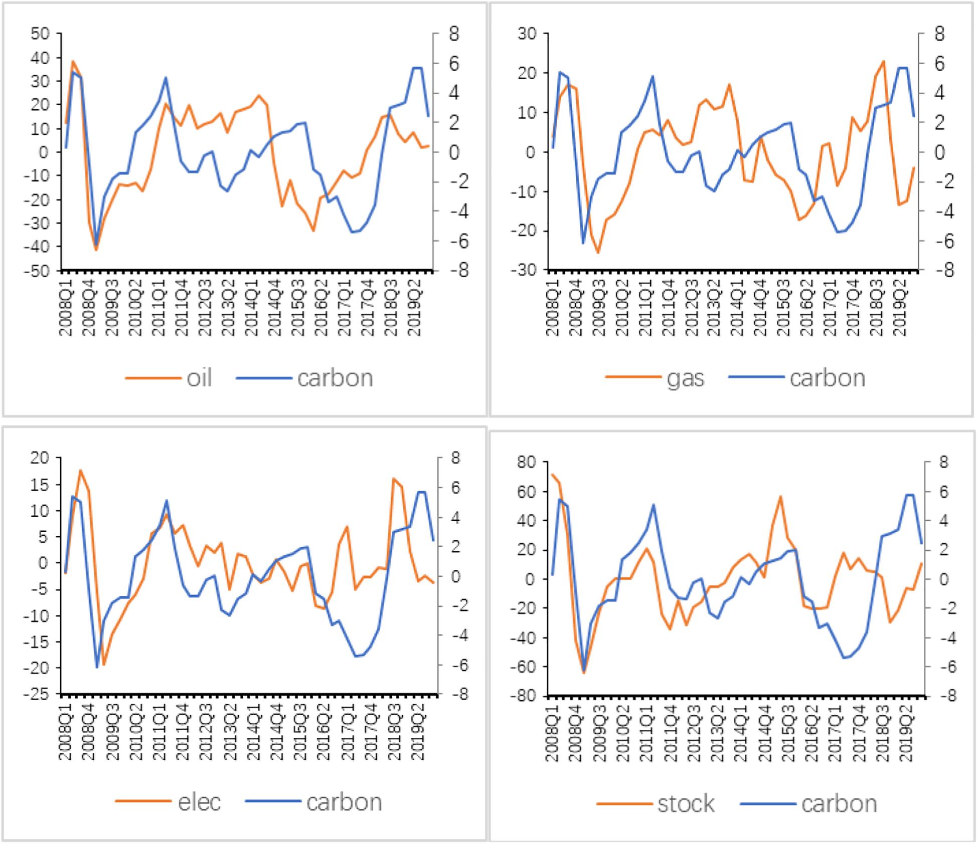
Figure 1. Carbon price (thick solid line) and key price drivers (thin solid line) periodic series.
Judgment of Time-Varying Characteristics of Variables
The EU ETS entered the third phase on January 1, 2013. Compared with the previous two stages, the quota allocation policy in the third stage has undergone major adjustments. As can be seen from Figure 1, the trends between oil, gas, electricity, stock prices and carbon price began to deviate to a certain extent inversion after 2013. Among them, the Paris Agreement adopted in December 2015 and signed in April 2016 amplified this inversion. The above phenomenon fully reflects the time-varying characteristics, which also indicates the applicability of using the time-varying parameter vector autoregressive (TVP-VAR) model. Meanwhile, this also provides a basis for us to select specific time points in the first quarter of 2013 and the quarter of 2016 for more detailed analysis.
Model Setting and Parameter Diagnosis
Based on the above analysis, this study establishes a TVP-VAR model that includes carbon, oil, gas, electricity, and stock prices. The following priors are assumed for the i-th diagonals of the covariance matrices:
For the initial state of the time-varying parameters, μβ0 = μa0 = μh0 = 0 and ∑β0 = ∑a0 = ∑h0 = 10×I. We use the MCMC method to simulate 20,000 times to obtain valid samples. The lags are determined by the estimated marginal likelihood and the invalid influence factor. We estimate the model with one to six lags and choose the lags in which marginal likelihood is the highest. Finally, the empirical result indicates the most fitted is one lag. The TVP-VAR estimation often needs many lags, because the shocks in the economic variables are considered to affect the other variables of the system with a delay. Figure 2 shows the sample autocorrelation function, the sample paths, and the posterior densities for selected parameters. It can be seen from Figure 2, the sample paths are stable and the sample autocorrelations drop stably, indicating the MCMC method with preset parameters efficiently produces uncorrelated samples.
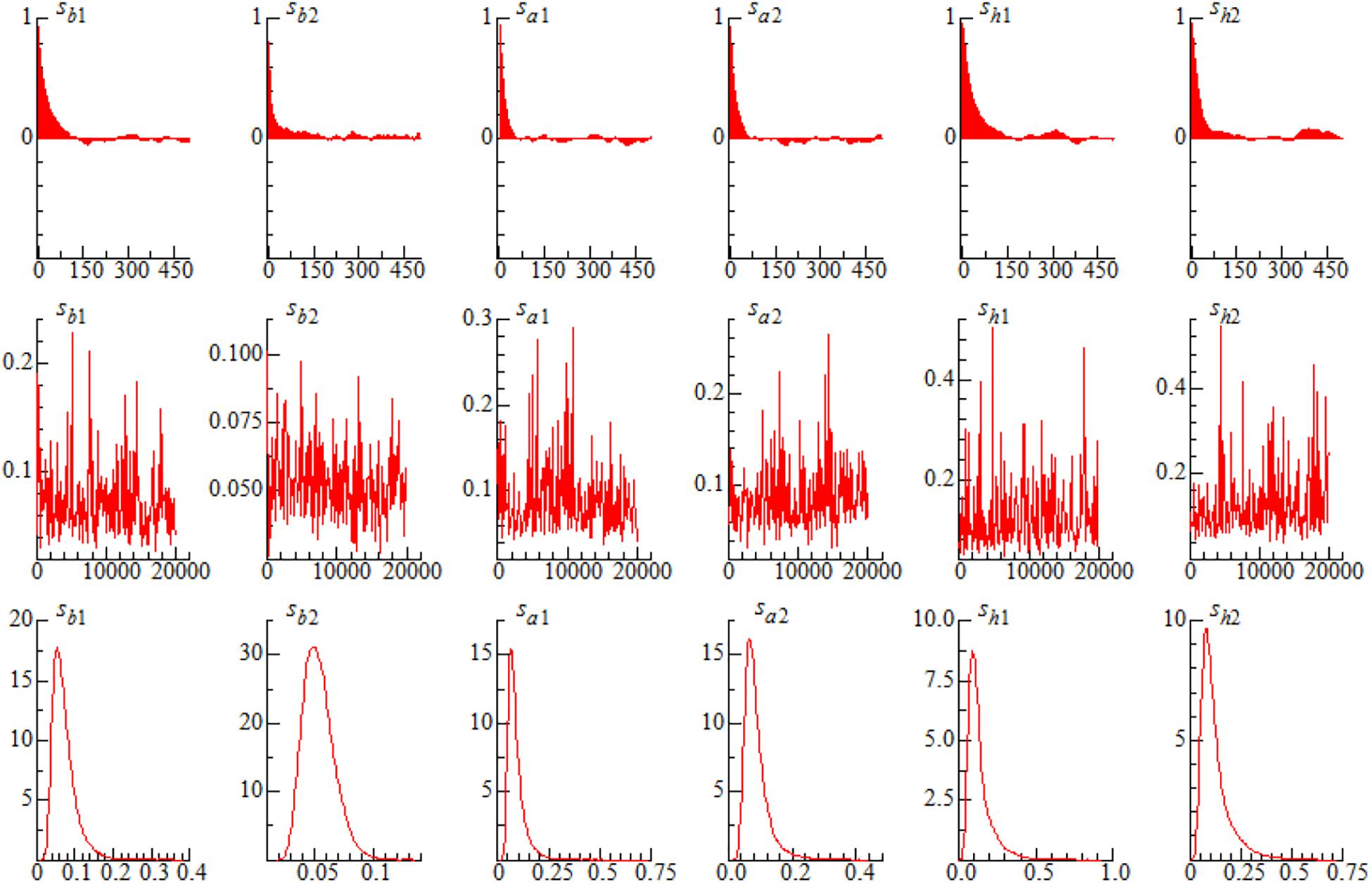
Figure 2. Sample autocorrelations (top), sample paths (middle), and posterior densities (bottom).
Estimation Results of Model Parameters
Before estimating, we conduct a stationary test on each variable, and the results show that each variable is stable at the 5% level. Table 1 provides the estimation results. The standard deviations of the parameters are relatively small, and the posterior mean values are all within the 95% confidence interval. Judging from the convergence, the Geweke values of the parameters does not exceed the critical value of 1.96 at the 5% significance level, indicating that the null hypothesis of “parameters converging to the posterior distribution” cannot be rejected. The inefficiency factor is an index to measure the effectiveness of sampling. It is used to calculate the number of uncorrelated samples that can be obtained under a given sampling frequency. The smaller the inefficiency factor is, the more effective the sampling is. It can be seen from Table 1 that the inefficiency factor of each parameter is much smaller than the number of sampling times 20,000, of which the maximum value is about 65. This means that in the case of continuous sampling of 20,000 times, we can obtain at least about 307 uncorrelated samples, which can meet the needs of model estimation.
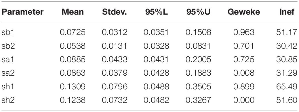
Table 1. Estimation results for selected parameters in the TVP-VAR model.
Empirical Analysis Results
Time-Varying Stochastic Volatility Analysis
(A) Carbon and Oil Price
The time-varying stochastic volatilities of carbon price and different driving factors are shown in Figure 3. In terms of carbon and oil prices, the response of carbon price to oil price shocks was negative before 2015, and as the number of the lag increased, the degree of response increase as well, which is consistent with Rickels et al. (2014). This result is not surprising, since rising oil price tends to reduce economic growth (Lardic and Mignon, 2008), which in turn reduces energy consumption and the demand for carbon allowances, thereby lowering carbon price. After 2016, the response of carbon price to oil price shocks clearly turned positive, and the response value continually increased. This may be due to the substitution effect of the oil. When the oil price rises, people tend to increase the use of alternative energy with lower prices and higher carbon emission intensity, such as coal, which leads to the increase of carbon emissions, an increase of carbon quota demand, and a rise of carbon price.
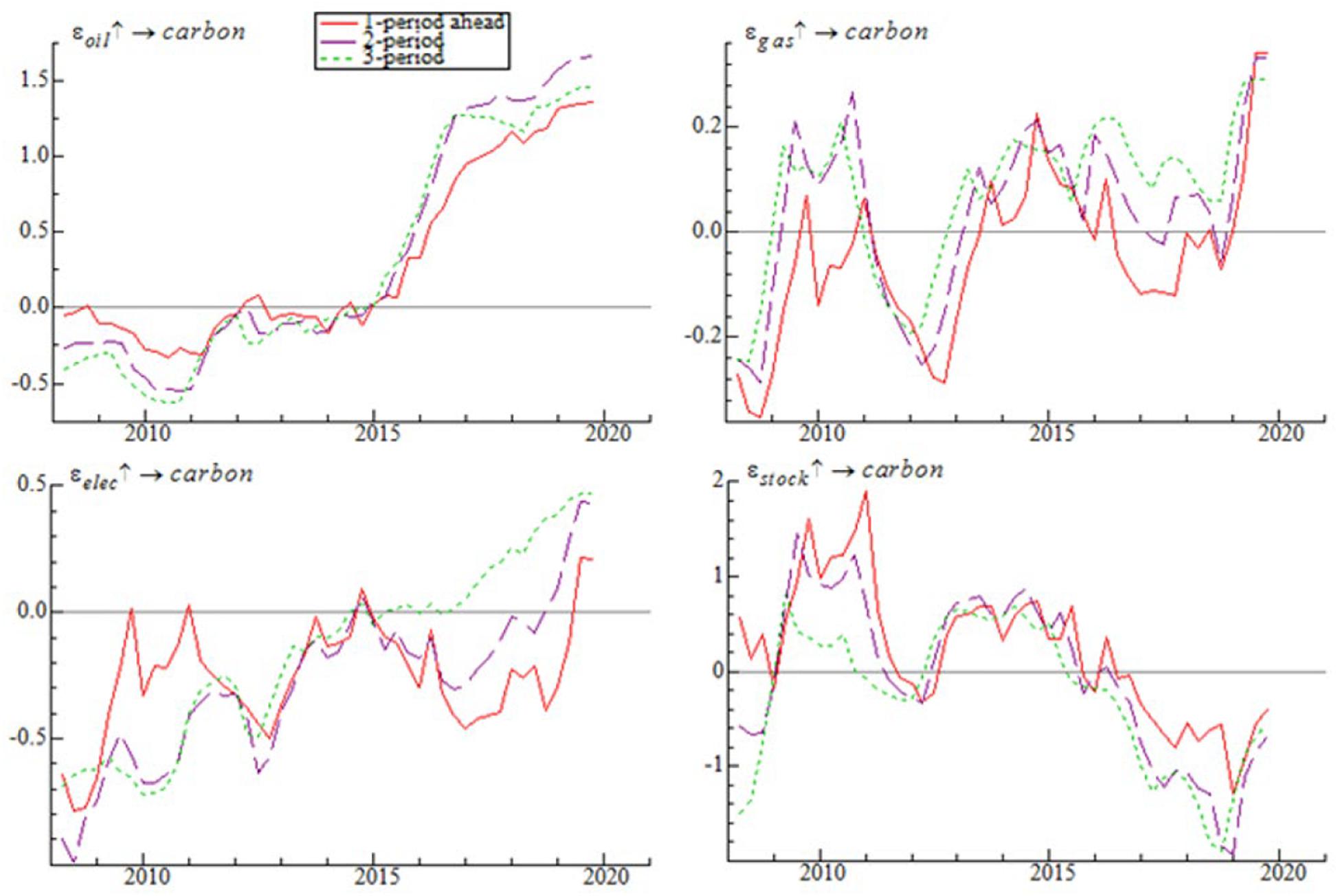
Figure 3. Time impulse graph of the impact of carbon price on key price drivers.
(B) Carbon and Gas Price
In terms of carbon price and gas price, the response of carbon price to gas price shocks was almost negative in 1 lag, negative in the main parts of lag 2 and 3 before 2013. This is consistent with Zhang and Wei (2010). From 2013 to the first half of 2016, the response of carbon price to gas price shocks was positive in each lag. This might be because the increase in gas price encouraged people to use lower-priced energy such as oil and coal, which have higher emission intensity; thereby it would increase carbon emissions and push up carbon price. Starting from the second half of 2016, the response of carbon price to gas price shocks turns to negative in lag 1. After the signing of the Paris Agreement, clean energy started to develop rapidly, and electric power companies could also receive certain compensation for using clean energy. This may have caused electric power companies to increase the consumption of clean energy in the short-term to replace the gas, thereby reducing carbon emissions and carbon price.
(C) Carbon and Electricity Price
The response of carbon price to electricity price shocks was negative before 2016. The response of carbon price to electricity price shocks first turned positive in lag 3 at the end of 2016. The negative correlation between electricity price and carbon price before 2016 is consistent with the results of Hammoudeh et al. (2014). After 2016, when electricity price rise, the electric power companies will increase power generating capacity, which will increase carbon emissions and carbon price. In that scenario, there is a positive correlation between electricity price and carbon price (Zhu et al., 2019).
(D) Carbon and Stock Price
The response of carbon price to stock price shocks was positive, and the response peak value decreased before 2016. The short-term impact of stock price on carbon price was greater than the medium-term impact. After 2016, the response of carbon price to stock price shocks was negative, and the response peak value increased. The short-term (1 quarter) impact of stock price on carbon price was smaller than the mid-term (2 quarters) impact. Considering the two rounds of carbon price increase before 2016 and the first round of decline after 2016 in Figure 1, the response of carbon price to stock price shocks was positive in each lag, and the response value of lags 3 was the smallest during the first round of carbon price increases between 2009 and 2011; while the response of carbon price to stock price shocks was also positive in each lag, and the response values in lag 1, 2, and 3 were of the same level during the second round of carbon price increases from 2013 to the end of 2015. During the carbon price declines in 2016 and the first half of 2017, the impact of carbon price on stock price was negative in each lag, and the absolute value of the response value in lag 1 was the smallest. It is noticeable that the response of carbon price to stock price shocks changed from positive to negative is related to clean energy. After the European debt crisis, the EU issued a financial rescue package in July 2012, and European countries emerged from the crisis quagmire one after another. The recovery of the EU’s economy was manifested by the rise in stock price, which indicated people’s expectation that the economy was improving. Therefore, investors increased investment, residents increased consumption, and enterprises expanded production. These lead to an increase in carbon emissions, greater demand for carbon allowances, and higher carbon price (Lutz et al., 2013; Zhu et al., 2019). Subsequently, European stock markets experienced a relatively sharp decline in 2015 and began gradually recovering in 2016, signaling a positive economy, and indecisive investors entered the stock market. During this period, the low-carbon economy and sustainable development attracted widespread attention. Especially after the signing of the Paris Agreement, most of the EU countries formulated new policies in order to realize the EU 20-20-20 targets. These policy goals will greatly reduce the investment risk of renewable energy, thereby promoting the flow of funds to the low-carbon economy (Monasterolo and Angelis, 2020; Glavas, 2020), and the stock market could be a financing resource for renewable energy (Ji and Zhang, 2019). At the same time, the implementation of emission reduction policies will strengthen residents’ low-carbon awareness and increase the use of low-carbon transportation and products (Gallagher and Muehlegger, 2011; Cohen et al., 2015; Wen et al., 2018). This might be the reason carbon price responded negatively to stock price shocks after 2016.
Full-Sample Time-Varying Impulse Analysis
In order to obtain a more robust result, Figure 4 shows the three-dimensional impulse response of carbon price to oil and gas prices, which is the driver of carbon price, at different time points and in different lags. The three-dimensional impulse response graph can more clearly illustrate the extent of impacts of the drivers on carbon price and the term structure of the impacts.
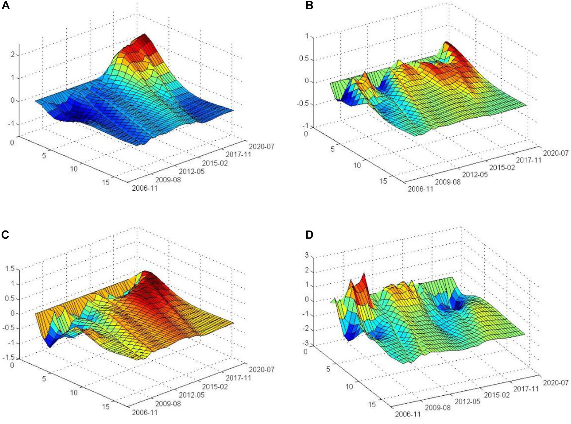
Figure 4. Full sample impulse graph of the impact of carbon price on key price drivers. (A) Full sample impulse of carbon price response to oil price shocks. (B) Full sample impulse of carbon price response to gas price shocks. (C) Full sample impulse of carbon price response to electricity price shocks. (D) Full sample impulse of carbon price response to stock price shocks.
(A) Carbon and Oil Price
The response of carbon price to oil price shocks varied significantly from negative to positive, with the inversion point roughly occurring in 2016. Before 2016, the impact of oil price on carbon price was negative in each lag. After that year, the positive response peaks increased continuously. Judging from the degree of impact, the negative response peaked approximately in lag 3, while the positive response peaked approximately in lag 2.
(B) Carbon and Gas Price
The response of carbon price to gas price shocks alternated between positive and negative. After 2013, the response of carbon price to gas price shocks was positive in almost each lag, with only lag 1 exhibiting a negative value for a longer span after 2016. In terms of the degree of impact, the response of carbon price to gas price shocks fluctuated slightly. In comparison, the fluctuations were larger before 2013 and tended to be flat after 2013. Both positive and negative response peaks appeared in lag 1.
(C) Carbon and Electricity Price
The response of carbon price to electricity price shocks changed from negative to positive, with the inversion point occurring earlier as the lag increased. In other words, the inversion point of lag 3 was roughly located in 2016, while the inversion point of lag 4 was roughly located in 2014. Meanwhile, judging from the changing trend of their relationship throughout the entire sample period, as the lag increases, the response of carbon price to the electricity price shocking are also changing from negative to positive. The impact of electricity price on carbon price was almost entirely negative in lag 1. When the lag was approximately greater than 5, the impact of electricity price on carbon price was almost completely positive, eventually approaching zero as the lag increased. In terms of the degree of impact, the negative response roughly peaked in lag 2, while the positive response roughly peaked in lag 3.
(D) Carbon and Stock Price
The response of carbon price to stock price shocks clearly changed from positive to negative, with the inversion point roughly occurring in 2016. Prior to this, the response of carbon price to stock price shocks was positive, but after 2016, the response of carbon price to stock price shocks was consistently negative. Judging from the degree of impact, the inversion of the positive response after 2013 was smaller, although there was no inversion. The positive response peaked in lag 1, while the negative response roughly peaked in lag 4. It can be seen that before the inversion point, the short-term impact of stock price on carbon price was greater than the mid-long term impact. After the inversion point, the short-term impact of stock price on carbon price was smaller than the medium and long-term impact. This may be related to the effective time of the policy and the ability of stock prices of different maturities to digest policy information. In other words, the short-term effect of economic stimulus policies is greater than the mid-long term effect, while the mid-long term effect of renewable energy development policies may be more obvious. At the same time, stock price can reflect more policy information in the mid-long term.
In general, the response of carbon price to key price drivers has changed over time, and the direction of the response underwent an inversion in 2016. Carbon price were more sensitive to changes in oil, gas, electricity, and stock prices before the inversion in short term, while their responses to changes in stock price after the break were more obvious in the mid-long term. In addition, the magnitude of carbon price response to oil price shocks and stock price shocks was larger, followed by electricity price, while gas price had the smallest magnitude of response. This shows that oil and stock prices have the greatest impact on carbon price, followed by electricity price and gas price (the smallest one).
Time-Point Time-Varying Impulse Analysis
Considering the adjustment of the quota allocation policy in the third phase of carbon emissions trading and the impact of the Paris Agreement on the EU ETS, we selected two specific time points for impulse analysis; the first one is in the first quarter of 2013 and the other is in the second quarter of 2016. At these two different time points, each variable was given a positive shock of standard deviation, and the responses of carbon price to oil, gas, and electricity prices exhibited similar trends at the two time points, while the responses of carbon price to the stock price shocks displayed significantly different and opposite trends at the two time points (see as Figure 5).
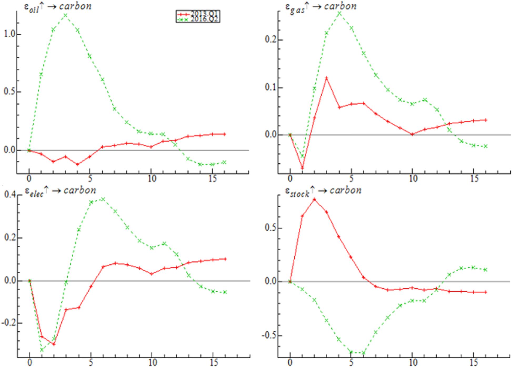
Figure 5. Time-point impulse graph of the impacts of carbon price on key price drivers.
(A) Carbon and Oil Price
In terms of the responses associated with carbon and oil prices, in the first quarter of 2013, the response value of carbon price to oil price shocks fluctuated within a small range around zero, was negative before lag 6, weakened in lag 3, and was positive after lag 6. In the second quarter of 2016, the response value of carbon price to oil price shocks changed from positive to negative, and the fluctuation range was [-0.10, 1.20]. It reached a positive peak of 1.20 in lag 3, then beginning to decrease and turning to negative in lag 13.
(B) Carbon and Gas Price
In terms of the responses associated with carbon and gas price, in the first quarter of 2013, the response value of carbon price to gas price shocks changed from negative to positive, and the fluctuation range was [−0.07, 0.12]. It reached a negative peak of −0.07 in lag 1, then beginning to rise, and turning to positive in lag 2. In the second quarter of 2016, the response value of carbon price to gas price shocks also changed from negative to positive, and the fluctuation range was [−0.04, 0.26]. It reached a negative peak of −0.04 in lag 1 and beginning to rise following a positive turning in lag 2.
(C) Carbon and Electricity Price
In terms of the responses associated with carbon and electricity price, in the first quarter of 2013, the response value of carbon to electricity price shocks changed from negative to positive, and the fluctuation range was [−0.30, 0.12]. It reached a negative peak of −0.30 in lag 2, then beginning to rise and experiencing a turnover impact in lag 6. In the second quarter of 2016, the response value of carbon to electricity price shocks also changed from negative to positive, and the fluctuation range was [−0.32, 0.26]. It reached a negative peak of −0.32 in lag 1 and experienced a turnover in lag 4.
(D) Carbon and Stock Price
In terms of responses associated with carbon and stock price, in the first quarter of 2013, the response value of carbon to stock price shocks changed from positive to negative with a positive in lag 2 and a turnover in lag 7, and the fluctuation range was [−0.10, 0.85]. In the second quarter of 2016, the response value of carbon to stock price shocks changed from negative to positive, and the fluctuation range was [−0.65, 0.15]. It reached a negative peak of −0.65 in lag 5 and it turning to the opposite in lag 13.
Additionally, compared with the first quarter of 2013, the response magnitude of carbon price to various shocks increased significantly after the second quarter of 2016. This indicates that carbon price became more sensitive to changes in its driving factors after the adoption of the Paris Agreement. That is, the information transmission between the carbon market and other markets is more obvious (Naeem et al., 2020). Furthermore, the absolute value of the response to changes in carbon price caused by changes in oil price was the largest, approaching 1.20, i.e., carbon price is more sensitive to changes in oil price, and followed by stock price, and finally electricity price and gas price when judging by the level of the response value.
Conclusions and Discussions
Carbon price is influenced by international environments, EU energy development plans and carbon emission reduction situations, and EU ETS policy design and expectations, all of these factors may lead to changes in the correlations between variables. Therefore, this study uses the TVP-VAR model to analyze the time-varying impacts of oil, gas, electricity, and stock prices on carbon price.
Firstly, there was an inversion in the impacts of different price drivers on carbon price in 2016. As for oil, the higher price initially tended to inhibit economic growth and reduced carbon emissions and carbon price. After 2016, the positive response of carbon price to oil price shocks is more obvious. As for the electricity, the increased price may not have prompted power companies to increase the generating capacity before 2016. At the same time, the increase in electricity price reduces the demand for electricity, thereby reducing carbon emissions and carbon price. After 2016, the increase in electricity price may increase the supply of electricity. As for stock price, the recovery of the EU’s economy was manifested by the rise in stock price after the European debt crisis. This led to an increase in carbon emissions and greater demand for carbon allowances which cause higher carbon price. After the signing of the Paris Agreement, the EU is affected by more sustainable development policies and a low-carbon economy. These may reduce carbon emissions and lower carbon price.
Secondly, full-sample time-varying impulse analysis revealed that the short-term impacts of the stock price before the inversion, oil, gas, and electricity prices on carbon price were greater than the mid-long term impacts, while the short-term impact of the stock price after the inversion on carbon price was less than the mid-long term impact. This may be related to the effective time of the policy and the ability of stock prices of different maturities to digest policy information. In addition, oil and stock price were found to exert a greater impact on carbon price.
Thirdly, this paper discovered that the direction of the impact of stock price on carbon price underwent more obvious changes when comparing with other carbon price influencing factors after the second quarter of 2016. In addition, compared with the level of response in the first quarter of 2013, carbon price had a greater magnitude of response to changes in their driving factors after the second quarter of 2016. Among them, carbon price exhibited the strongest response to changes in oil price, and the fluctuation range was [−0.10, 1.20]. It reached a positive peak of 1.20 in lag 3. That is, the oil market has the greatest impact on the carbon market (Ji et al., 2018b; Wang and Guo, 2018).
The results of this research may have practical implications for the optimal investment portfolio allocation, carbon price prediction, and risk management of financial market participants. To make a better hedging strategy, investors holding assets and derivatives in the carbon market should pay close attention to changes in the oil, gas, electricity, and stock markets especially change in oil price and also pay attention to short- and long-term policy trends. Industrial emission companies can adjust their energy consumption structure in a timely manner based on the time-varying relationship between the carbon market and the energy market to achieve the optimal carbon emission reduction strategy. Moreover, under structural policies such as high energy efficiency and clean energy use, economic growth and reduction of carbon dioxide emissions can be achieved at the same time (Chiu, 2016; Acheampong, 2018). Finally, this study also shows that the conclusions on carbon price drivers in the first and second phases of EU ETS are not fully applicable in the third phase.
This study has certain limitations: (1) Subject to the constraints of the TVP-VAR method, it may be difficult to capture the shorter-term impacts from analysis using quarterly frequency data, although this will not affect the robustness of the analysis. The comparison between the results of the constant parameter model based on sub-samples or rolling samples and the TVP-VAR model is still worthy of further study. (2) When analyzing the impact of stock price on carbon price, this study did not classify the stock index in a more detailed manner. (3) Since the index related to clean energy cannot effectively reflect the true development level of clean energy in the EU and its substitution for traditional fossil energy sources, therefore, the index is not included in the time-varying model used in this study.
Data Availability Statement
The original contributions presented in the study are included in the article/supplementary material, further inquiries can be directed to the corresponding author/s.
Author Contributions
PL did the model, the first draft, and modification. HZ did the data, the first draft, and modification. YY did the idea, writing the introduction, and modification of the draft. AH modified the English version and the language. All authors contributed to the article and approved the submitted version.
Conflict of Interest
The authors declare that the research was conducted in the absence of any commercial or financial relationships that could be construed as a potential conflict of interest.
Acknowledgments
We are grateful to the National Natural Science Foundation of China (NSFC Grant No. 71673263), the Fundamental Research Funds for the Central University, and support plan of the philosophy and social science innovation team in colleges and universities of Henan Province (2018-CXTD-06) for primary financial support of this work.
Footnotes
- ^ https://ec.europa.eu/clima/policies/ets/revision_en
- ^ What needs to be explained is the coal price factor. Some studies on the relationship between the carbon market and the energy market after the establishment of the EU ETS have found that Brent crude oil price has the largest contribution to carbon price, followed by gas, and coal has a relatively small contribution (Zhang and Wei, 2010; Ji et al., 2018b). At the same time, when we use the TVP-VAR model for fitting, we find that the impact of coal price on carbon price is not significant. Therefore, the coal price factor will not be considered in the model.
References
Aatola, P., Ollikainen, M., and Toppinen, A. (2013). Price determination in the EU ETS market: theory and econometric analysis with market fundamentals. Energy Econ. 36, 380–395. doi: 10.1016/j.eneco.2012.09.009
Acheampong, A. O. (2018). Economic growth, CO2 emissions and energy consumption: what causes what and where? Energy Econ. 74, 677–692. doi: 10.1016/j.eneco.2018.07.022
Ahmad, N., Du, L., Lu, J., Wang, J., Li, H. Z., and Hashmi, M. Z. (2017). Modelling the CO2 emissions and economic growth in Croatia: is there any environmental Kuznets curve? Energy 123, 164–172. doi: 10.1016/j.energy.2016.12.106
Alaa, M. S., and Muhammad, A. N. (2019). Association between the energy and emission prices: an analysis of EU emission trading system. Resour. Policy 61, 369–374. doi: 10.1016/j.resourpol.2018.12.005
Alberola, E., Chevallier, J., and Cheze, B. (2008a). Price drivers and structural breaks in European Carbon Prices 2005-2007. Energy Policy 36, 787–797. doi: 10.1016/j.enpol.2007.10.029
Alberola, E., Chevallier, J., and Chèze, B. (2008b). The EU emissions trading scheme: the effects of industrial production and CO2 emissions on carbon prices. Int. Econ. 116, 93–125. doi: 10.3917/ecoi.116.0093
Andreoni, V., and Galmarini, S. (2016). Drivers in CO2 emissions variation: a decomposition analysis for 33 world countries. Energy 103, 27–37. doi: 10.1016/j.energy.2016.02.096
Balcilar, M., Demirer, R., Hammoudeh, S., and Nguyen, D. K. (2016). Risk spillovers across the energy and carbon markets and hedging strategies for carbon risk. Energy Econ. 54, 159–172. doi: 10.1016/j.eneco.2015.11.003
Balcilar, M., Ozdemir, Z. A., and Arslanturk, Y. (2010). Economic growth and energy consumption causal nexus viewed through a bootstrap rolling window. Energy Econ. 32, 1398–1410. doi: 10.1016/j.eneco.2010.05.015
Batten, J. A., Maddox, G. E., and Young, M. R. (2020). Does weather, or energy prices, affect carbon prices? Energy Econ. 11:105016. doi: 10.1016/j.eneco.2020.105016
Boersen, A., and Scholtens, B. (2014). The relationship between European electricity markets and emission allowance futures prices in phase II of the EU (European Union) emission trading scheme. Energy Oxford 74, 585–594. doi: 10.1016/j.energy.2014.07.024
Bredin, D., and Muckley, C. (2011). An emerging equilibrium in the EU emissions trading scheme. Energy Econ. 33, 353–362. doi: 10.1016/j.eneco.2010.06.009
Chevallier, J. (2009). Carbon futures and macroeconomic risk factors: a view from the EU ETS. Energy Econ. 31, 614–625. doi: 10.1016/j.eneco.2009.02.008
Chevallier, J., Nguyen, D. K., and Carlos, R. J. (2019). A conditional dependence approach to CO2 -energy price relationships. Energy Econ. 81, 812–821. doi: 10.1016/j.eneco.2019.05.010
Chiu, Y. B. (2016). Carbon dioxide, income and energy: evidence from a non-linear model. Energy Econ. 61, 279–288. doi: 10.1016/j.eneco.2016.11.022
Cohen, M. C., Lobel, R., and Perakis, G. (2015). The impact of demand uncertainty on consumer subsidies for green technology adoption. Soc. Sci. Electron. Publish. 62, 868–878.
Creti, A., Pierre-André, J., and Valérie, M. (2012). Carbon price drivers: phase I versus Phase II equilibrium? Energy Econ. 34, 327–334. doi: 10.1016/j.eneco.2011.11.001
Daskalakis, G., Psychoyios, D., and Markellos, R. N. (2009). Modeling CO2 emission allowance prices and derivatives: evidence from the European trading scheme. J. Bank. Financ. 33, 1230–1241. doi: 10.1016/j.jbankfin.2009.01.001
Diebold, F. X., and Yilmaz, K. (2012). Better to give than to receive: predictive directional measurement of volatility spillovers. Int. J. Forecas. 28, 57–66. doi: 10.1016/j.ijforecast.2011.02.006
Fama, E. F., and French, K. R. (1987). Dividend yields and expected stock returns. J. Financ. Econ. 22, 3–25. doi: 10.1016/0304-405x(88)90020-7
Fan, J. H., Akimov, A., and Roca, E. (2013). Dynamic hedge ratio estimations in the European Union Emissions offset credit market. J. Clean. Prod. 42, 254–262. doi: 10.1016/j.jclepro.2012.10.028
Gallagher, K. S., and Muehlegger, E. (2011). Giving green to get green? Incentives and consumer adoption of hybrid vehicle technology. J. Environ. Econ. Manag. 61, 1–15. doi: 10.1016/j.jeem.2010.05.004
Glavas, D. (2020). Green regulation and stock price reaction to green bond issuance. Finance 41:7. doi: 10.3917/fina.411.0007
Gronwald, M., Ketterer, J., and Trück, S. (2011). The relationship between carbon, commodity and financial markets: a copula analysis. Econ. Record 87(Suppl. 1), 105–124. doi: 10.1111/j.1475-4932.2011.00748.x
Hammoudeh, S., Lahiani, A., Nguyen, D. K., and Sousa, R. M. (2015). An empirical analysis of energy cost pass-through to CO2 emission prices. Energy Econ. 49, 149–156. doi: 10.1016/j.eneco.2015.02.013
Hammoudeh, S., Nguyen, D. K., and Sousa, R. M. (2014). What explain the short-term dynamics of the prices of CO2 emissions? Energy Econ. 46, 122–135. doi: 10.1016/j.eneco.2014.07.020
Hintermann, B. (2010). Allowance price drivers in the first phase of the EU ETS. J. Environ. Econ. Manag. 59, 43–56. doi: 10.1016/j.jeem.2009.07.002
Ji, Q., Liu, B. Y., Zhao, W. L., and Fan, Y. (2018a). Modelling dynamic dependence and risk spillover between all oil price shocks and stock market returns in the BRICS. Int. Rev. Financ. Anal. 68:101238. doi: 10.1016/j.irfa.2018.08.002
Ji, Q., Zhang, D., and Geng, J. (2018b). Information linkage, dynamic spillovers in prices and volatility between the carbon and energy markets. Clean. Prod. 198, 972–978. doi: 10.1016/j.jclepro.2018.07.126
Ji, Q., and Zhang, D. (2019). How much does financial development contribute to renewable energy growth and upgrading of energy structure in China? Energy Policy 128, 114–124. doi: 10.1016/j.enpol.2018.12.047
Jimenez-Rodriguez, R. (2019). What happens tohappens to the relationship between EU allowances prices and stock market indices in Europe? Energy Econ. 81, 13–24. doi: 10.1016/j.eneco.2019.03.002
Keppler, J. H., and Mansanet-Bataller, M. (2010). Causalities between CO2, electricity, and other energy variables during phase I and phase II of the EU ETS. Energy Policy 38, 3329–3341. doi: 10.1016/j.enpol.2010.02.004
Koch, N., Fuss, S., Grosjean, G., and Edenhofer, O. (2014). Causes of the EU ETS price drop: recession, CDM, renewable policies or a bit of everything?-New evidence. Energy Policy 73, 676–685. doi: 10.1016/j.enpol.2014.06.024
Kumar, S., Managi, S., and Matsuda, A. (2012). Stock prices of clean energy firms, oil and carbon markets: a vector autoregressive analysis. Energy Econ. 34, 215–226. doi: 10.1016/j.eneco.2011.03.002
Lardic, S., and Mignon, V. (2008). Oil prices and economic activity: an asymmetric cointegration approach. Energy Econ. 30, 847–855. doi: 10.1016/j.eneco.2006.10.010
Liu, J. X., Zhang, Z. Y., and Zhang, Y. (2013). The relationship between carbon futures and energy stock prices and its policy implications for China — Take the EU as an example. Econ. 4, 43–55. doi: 10.16158/j.cnki.51-1312/f.2013.04.003
Liu, W. Q., and Zhao, J. (2011). Empirical research on spillover effect and dynamic correlation between EU ETS Future Market — Base on DCC-MVGARCH. Lanzhou Acad. J. 5, 37–41.
Lutz, B. J., Pigorsch, U., and Rotfuß, W. (2013). Nonlinearity in cap-and-trade systems: the EUA price and its fundamentals. Energy Econ. 40, 222–232. doi: 10.1016/j.eneco.2013.05.022
Mansanet-Bataller, M., Chevallier, J., Hervé-Mignucci, M., and Alberola, E. (2011). EUA and sCER phase II price drivers: unveiling the reasons for the existence of the EUA-sCER spread. Energy Policy 39, 1056–1069. doi: 10.1016/j.enpol.2010.10.047
Mansanet-Bataller, M., Pardo, A., and Valor, E. (2007). CO2 Prices, energy and weather. Energy J. 28, 73–92.
Maryniak, P., Truck, S., and Weron, R. (2019). Carbon pricing and electricity markets — The case of the Australian clean energy bill. Energy Econ. 79, 45–58. doi: 10.1016/j.eneco.2018.06.003
Monasterolo, I., and Angelis, L. D. (2020). Blind to carbon risk? An analysis of stock market reaction to the Paris Agreement. Ecol. Econ. 170:106571. doi: 10.1016/j.ecolecon.2019.106571
Muhammad, S., and Long, X. (2021). Rule of law and CO2 emissions: a comparative analysis across 65 belt and road initiative (BRI) countries. J. Clean. Prod. 279:123539. doi: 10.1016/j.jclepro.2020.123539
Naeem, M. A., Peng, Z., Suleman, M. T., Nepal, R., and Shahzad, S. J. H. (2020). Time and frequency connectedness among oil shocks, electricity and clean energy markets. Energy Econ. 91:104914. doi: 10.1016/j.eneco.2020.104914
Nakajima, J. (2011). Time-varying parameter VAR model with stochastic volatility: an overview of methodology and empirical applications. Mon. Econ. Stud. 29, 107–142.
Nakajima, J., Kasuya, M., and Watanabe, T. (2011). Bayesian analysis of time-varying parameter vector autoregressive model for the Japanese economy and monetary policy. J. Jpn. Int. Econ. 25, 225–245. doi: 10.1016/j.jjie.2011.07.004
Oberndorfer, U. (2008). EU Emission Allowances and the stock market: evidence from the electricity industry. SSRN Electron. J. 68, 1116–1126. doi: 10.1016/j.ecolecon.2008.07.026
Parry, I. (2020). Increasing carbon pricing in the EU: evaluating the options. Eur. Econ. Rev. 121:103341. doi: 10.1016/j.euroecorev.2019.103341
Peng, L. I., Du, Y., Mao, D., and Han, Q. (2015). Is inflation a fiscal phenomenon in China? a time-varying parameter study from perspective of fiscal expenditure. Financ. Trade Res. 26, 88–96.
Peri, M., and Baldi, L. (2011). Nonlinear price dynamics between CO2 futures and Brent. Appl. Econ. Lett. 18, 1207–1211. doi: 10.1080/13504851.2010.532092
Primiceri, G. E. (2005). Time varying structural vector autoregressions and monetary policy. Rev. Econ. Stud. 72, 821–852. doi: 10.1111/j.1467-937x.2005.00353.x
Reboredo, J. C., and Ugando, M. (2015). Downside risks in EU carbon and fossil fuel markets. Mathem. Comput. Simul. 111, 17–35. doi: 10.1016/j.matcom.2014.12.001
Rickels, W., Görlich, D., and Peterson, S. (2014). Explaining European emission allowance price dynamics: evidence from phase II. German Econ. Rev. 16, 181–202. doi: 10.1111/geer.12045
Rossi, B., and Inoue, A. (2012). Out-of-sample forecast tests robust to the choice of window size. J. Bus. Econ. Stat. 30, 432–453. doi: 10.1080/07350015.2012.693850
Sohag, K. (2015). Dynamics of energy use, technological innovation, economic growth and trade openness in Malaysia. Energy 90(Pt. 2), 1497–1507. doi: 10.1016/j.energy.2015.06.101
Sousa, R., Aguiar-Conraria, L., and Soares, M. J. (2014). Carbon financial markets: a time–frequency analysis of CO2 prices. Physica A Stat. Mech. Appl. 414, 118–127.
Sousa, R., and Conraria, L. A. (2014). Dynamics of CO2 Price Drivers. NIPE Working Papers. Guimarães: NIPE - Universidade do Minho.
Tan, X., Sirichand, K., Vivian, A., and Wang, X. (2020). How connected is the carbon market to energy and financial markets? A systematic analysis of spillovers and dynamics. Energy Econ. 90:104870. doi: 10.1016/j.eneco.2020.104870
Twomey, P. (2012). Rationales for additional climate policy instruments under a carbon price. Econ. Labor Relat. Rev. 23, 7–31. doi: 10.1177/103530461202300102
Wang, Y., and Guo, Z. (2018). The dynamic spillover between carbon and energy markets: new evidence. Energy 149, 24–33. doi: 10.1016/j.energy.2018.01.145
Wen, W., Zhou, P., and Zhang, F. (2018). Carbon emissions abatement: emissions trading vs consumer awareness. Energy Econ. 76, 34–47. doi: 10.1016/j.eneco.2018.09.019
Wesseh, P. K., Lin, B., and Atsagli, P. (2017). Carbon taxes, industrial production, welfare and the environment. Energy 123, 305–313. doi: 10.1016/j.energy.2017.01.139
Yu, L., Li, J., and Tang, L. (2015a). Dynamic volatility spillover effect analysis between carbon market and crude oil market: a DCC-ICSS approach. Int. J. Glob. Energy Issues 38, 242–256. doi: 10.1504/ijgei.2015.070265
Yu, L., Li, J., Tang, L., and Wang, S. (2015b). Linear and nonlinear Granger causality investigation between carbon market and crude oil market: a multi-scale approach. Energy Econ. 51, 300–311. doi: 10.1016/j.eneco.2015.07.005
Zhang, Y. J., and Huang, Y. S. (2015). The multi-frequency correlation between EUA and sCER futures prices: evidence from the EMD approach. Fractal 23, 1–18.
Zhang, Y. J., and Sun, Y. F. (2016). The dynamic volatility spillover between European carbon trading market and fossil energy market. J. Clean. Prod. 112, 2654–2663. doi: 10.1016/j.jclepro.2015.09.118
Zhang, Y. J., and Wei, Y. M. (2010). Interpreting the complex impact of fossil fuel markets on the EU ETS futures markets: an empirical evidence. Manag. Rev. 21, 34–41.
Zhu, B., Ye, S., Han, D., Wang, H., He, K., Wei, Y. M., et al. (2019). A multiscale analysis for carbon price drivers. Energy Econ. 78, 202–216. doi: 10.1016/j.eneco.2018.11.007
Appendix
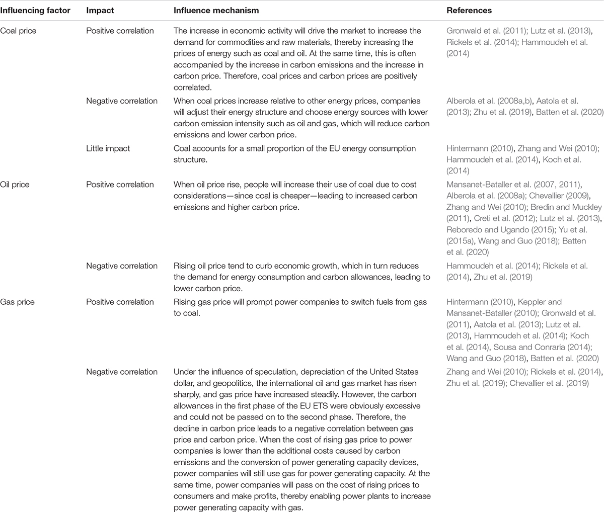
Table A1. Research on the relationship between the fossil energy market and carbon price.
Keywords: carbon price, a TVP VAR model, carbon price drivers, EU ETS, Paris agreement
Citation: Li P, Zhang H, Yuan Y and Hao A (2021) Time-Varying Impacts of Carbon Price Drivers in the EU ETS: A TVP-VAR Analysis. Front. Environ. Sci. 9:651791. doi: 10.3389/fenvs.2021.651791
Received: 11 January 2021; Accepted: 17 March 2021;
Published: 16 April 2021.
Edited by:
Syed Jawad Hussain Shahzad, Montpellier Business School, FranceReviewed by:
Mobeen Rehman, Shaheed Zulfiqar Ali Bhutto Institute of Science and Technology, PakistanMuhammad Abubakr Naeem, Massey University Business School, New Zealand
Copyright © 2021 Li, Zhang, Yuan and Hao. This is an open-access article distributed under the terms of the Creative Commons Attribution License (CC BY). The use, distribution or reproduction in other forums is permitted, provided the original author(s) and the copyright owner(s) are credited and that the original publication in this journal is cited, in accordance with accepted academic practice. No use, distribution or reproduction is permitted which does not comply with these terms.
*Correspondence: Yongna Yuan, anVsaWF5bnlAdWNhcy5hYy5jbg==