 Shanshan Zhao
 Wenping He3*
- 1National Climate Center, China Meteorological Administration, Beijing, China
- 2Collaborative Innovation Center on Forecast and Evaluation of Meteorological Disasters, Nanjing University of Information Sciences and Technology, Nanjing, China
- 3School of Atmospheric Sciences, Key Laboratory of Tropical Atmosphere-Ocean System (Sun Yat-sen University), Ministry of Education, Southern Marine Science and Engineering Guangdong Laboratory (Zhuhai), Zhuhai, China
- 4Chongqing Climate Center, Chongqing Meteorological Bureau, Chongqing, China
- 5Yangzhou Meteorological Office, Yangzhou, China
The daily average land surface air temperature (SAT) simulated by 8 CMIP5 models historical experiments and that from NCEP data during 1960–2005, are used to evaluate the performance of the CMIP5 model based on detrended fluctuation analysis (DFA) method. The DFA results of NCEP data show that SAT in most regions of the world exhibit long-range correlation. The scaling exponents of NCEP SAT show the zonal distribution characteristics of larg in tropics while small in medium and high latitudes. The distribution characteristics of the zonal average scaling exponents of CMCC-CMS, GFDL-ESM2G, IPSL-CM5A-MR are similar to that of NCEP data. From the DFA errors of model-simulated SAT, the performance of IPSL-CM5A-MR is the best among the 8 models throughout the year, the performance of FGOALS-g2 is good in spring and summer, GFDL-ESM2G is the best in autumn, CNRM-CM5 and CMCC-CMS is good in winter. The scaling exponents of model-simulated SAT are closer to that of NCEP data in most areas of the mid-high latitude on the northern hemisphere. However, simulations of SAT in East Asia and Central North American are generally less effective. In spring, most models have better performance in Siberian (SIB), Central Asia (CAS) and Tibetan (TIB). SAT in Northern Europe area are well simulated by most models in summer. In autumn, areas with better performance of most models are Mediterranean, SIB and TIB regions. In winter, SAT in Greenland, SIB and TIB areas are well simulated by most models. Generally speaking, the performance of CMIP5 models for SAT on global continents varies in different seasons and different regions.
Introduction
Climate system models are important tools for simulating climate systems and projecting future climate change (Phillips and Gleckler, 2006; Zhou and Yu, 2006; Flato et al., 2013). Assessment of model simulation performance can help us understand the advantages and disadvantages of the models, so as to provide a basis for users to choose models suitable for different purposes, and provide a scientific reference for model community to improve the performance of the models (Watterson et al., 2014). Coupled Model Intercomparison Project-Phase 5 (CMIP5) provides the dataset produced by multiple climate system models or earth system models (Taylor et al., 2012), which promotes the development of models themselves and the evaluation methods for model performance. The evaluation methods for model performance concentrate more on quantitative assessment than before, and emphasize the model evaluation criteria (Kharin et al., 2013; Elguindi et al., 2014; Sillmann et al., 2014). Most of these methods evaluate the outputs of multi-models on variant timescales, focusing on the climate states, climate change, or variations of indexes computed by meteorological elements (Sillmann et al., 2013; Yin et al., 2013; Jiang et al., 2016; Li et al., 2017), and provide the quantitative results of the differences between the model simulations and observations. However, the performance of models on simulating the intrinsic dynamical characteristics of climate system is rarely evaluated.
Climate systems are characterized by long-range correlation (LRC), which represents the self-similarity of climate evolution on different time scales (Bunde and Havlin., 2002; Bunde et al., 2005; Yuan et al., 2015; Fu et al., 2016a, 2016b; He et al., 2016). LRC has been found in meteorological observations, such precipitation (Kantelhardt et al., 2006) and as daily air temperature (Koscielny-Bunde, et al., 1996; Talkner and Weber, 2000; Gan et al., 2007; Jiang et al., 2015). LRC can be characterized by the power law of an autocorrelation coefficient (Beran, 1994). Some research pointed out that scaling exponents for daily air temperature were about universal over the continent (Koscielny-Bunde et al., 1998; Eichner et al., 2003). Weber and Talkner (2001) found LRC of daily air temperature depends on the altitude of the meteorological station. Király and Jánosi (2005) found that the scaling exponents of daily temperature over Australia were related with the geographic latitude, which exhibit a decrease tendency with increasing distance from the equator.
Detrended fluctuation analysis (DFA) is a well-known method to detect LRC in time series (Peng et al., 1994; Bunde and Havlin, 2002), and has been used to assess the capability of climate system models (Blender and Fraedrich, 2003; Kumar et al., 2013; Zhao and He, 2015; He and Zhao, 2018). Govindan et al. (2004) found that seven atmosphere-ocean general circulation models failed to reproduce the LRC of daily maximum temperature. Rybski et al. (2008) analyzed the LRC of daily temperature from historical simulation of global coupled general circulation model, and found that scaling exponents over most continent sites ranges from 0.6 to 0.8. By comparing the LRC with daily observational data over China, the performance of Beijing Climate Center Climate System Model 1.1(m) is systematically evaluated by using DFA methods (Zhao and He, 2014; Zhao and He, 2015). Therefore, it is a very well way to quantitatively evaluate the performance of climate model based on LRC of climate systems.
Because the spatial coverage of meteorological observation data is limited and varies with time, it is crucial to carry out homogenization and quality control of observational data. Reanalysis data can provide a set of meteorological data that is homogeneous in time and space (Marques et al., 2010). The National Centers for Environmental Prediction (NCEP) reanalysis data (Kalnay, 1996; Kanamitsu et al., 2002) is commonly used in climate research (Ma et al., 2008; Mooney et al., 2011). The quality of NCEP reanalysis datasets has been assessed on global and regional scales (Poccard et al., 2000; Josey, 2001; Mooney et al., 2011). He et al. (2018) showed that the daily average temperature from NCEP-2 and CFSR data exhibit LRC characteristics in China, which are similar to the results of observations, especially in central and eastern Northwest China, most of central and eastern China. Furthermore, the credibility of NCEP-2 and CFSR seasonal temperature were evaluated by DFA in China (Zhao et al., 2017). Based on this, we quantitatively evaluate the performance of CMIP5 models in simulating LRC of global daily land surface air temperature (SAT) by means of comparing the difference with LRC of NCEP-2 data in this study.
In this paper, DFA was used to evaluate the performance of CMIP5 models in simulating the global daily land SAT on a seasonal scale. The remainder of the present paper is organized as follows. Methods and Data briefly introduces the NCEP-2 data and the CMIP5 models used in this study, and then, the algorithm of the DFA is provided. In LRC of Daily Average SAT Simulated by Multi-Models, the LRC of the output datasets for all four seasons from CMIP5 models is analyzed by using DFA. Comparisons of the spatial differences of LRC between simulations and reanalysis data are also presented in this section. Conclusion summarizes the main results and conclusions of the present study with a brief discussion.
Methods and Data
Data
The global daily average land SAT from 1960 to 2005 is available from NCEP reanalysis dataset. The simulated global daily average land SAT is from the present-day historical simulations performed by the 8 CMIP5 climate models. The basic information about the 8 global climate models (GCM) is provided in Table 1. The term “historical” (HIST) refers to coupled climate model simulations forced by observed concentrations of greenhouse gases, solar forcing, aerosols, ozone, and land-use change over the 1850–2005 period (Taylor et al., 2012). The qualities of the past 46 years (1960–2005) data from the selected CMIP5 models were evaluated. To facilitate the intercomparison of the selected models and evaluation of the performance of 8 models against the NCEP data, the daily fields of GCM temperature were remapped onto T62 Gaussian grid from their original spatial resolution based on Ordinary Kriging (Mueller et al., 2004), which is the same as the spatial resolution of the reanalysis data, 2.5° × 2.5 ° resolution horizontal grid.
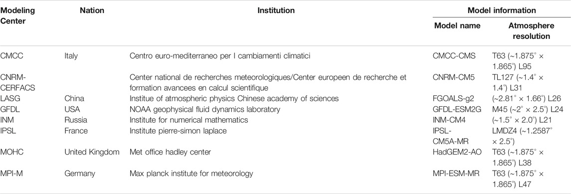
TABLE 1. Information about the eight CMIP5 climate models.
To disclose the geographical heterogeneity of DFA for the daily air temperature in the continents, we divided the continents into 22 sub-continental land regions (Table 2 and Figure 1), which are defined based on the literatures (Giorgi, 2002; Sillmann et al., 2013; Chan and Wu, 2015). The regions vary from a few thousand to several thousand km in each direction and cover global land areas with simple shape. The selection of specific regions was intended to represent climatic regimes and physiograhic settings (Giorgi, 2002). We calculated the area-averaged scaling exponents in each region for the daily SAT of NCEP and CMIP5 models, respectively. And then the differences of the area-averaged scaling exponents between the NCEP and model outputs were compared.
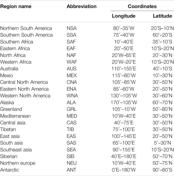
TABLE 2. Names and coordinates for the 22 regions in the continents.
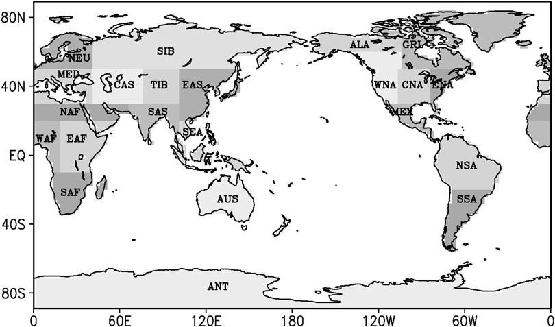
FIGURE 1. Divisions of the continents on earth.
Method
The DFA method can quantify LRC as an index, namely, scaling exponent (Peng et al., 1994). Consider a record of daily average temperature {Ti, i = 1, 2, …, N}, the multi-year mean daily average temperature
Then y(k) is divided into n = Int (
Typically,
If 1 > α > 0.5, the time series {Ti, i = 1, 2, …, N} is LRC. If α = 0.5, the time series is uncorrelated. If 0 < α < 0.5, the series {Ti} has anti-persistent correlation. When p = 2, a 2nd-order polynomial function is used to fit the profile y(k). DFA2 has been widely used in many researches. In this study, the DFA2 method is used to estimate the scaling exponent in a time series.
To estimate the uncertainties of the DFA2 method, we conducted six sets of independent tests for five given scaling exponents according to the reference (Zhao and He, 2015). In each test, 20,000 artificial time series were produced by Fourier-filtering method (Peng et al., 1991) with given scaling exponents varying from 0.6 to 1.0. Table 3 demonstrates the 2.5th and 97.5th percentiles for the DFA2’s estimated errors for each scaling exponent. Therefore, if the difference of LRC between the reanalysis data and the models is bigger than the estimated error of DFA2, the difference is statistically significant at a significance level of alpha = 0.05.
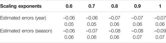
TABLE 3. The values in the 2.5th and 97.5th percentiles for DFA2’s estimated errors.
LRC of Daily Average SAT Simulated by Multi-Models
Characteristics of Daily Average SAT
As an example, one grid point (110°E, 23°N) located in the eastern part of Eurasia was randomly selected to show the LRC of SAT. The scaling exponent of NCEP SAT at this point is 0.6, which indicates a LRC. The scaling exponents of SAT at this point simulated by 8 CMIP5 models range from 0.52 to 0.74, which are quite different from the long-term correlation of the NCEP SAT (Figure 2A). Except for INM-CM4, the scaling exponents of SAT simulated by the models are bigger than those of NCEP SAT (Figure 3). As far as scaling exponents of SAT at the selected point are concerned, the differences between the most of CMIP5 simulations and NCEP data are greater than the uncertainties of the DFA2 calculation at a significance level of alpha = 0.05, except for IPSL-CM5A-MR. This means that only IPSL-CM5A-MR can relatively reliably reproduce the LRC of SAT of the selected point. In spring, scaling exponent of NCEP SAT at the grid point is 0.61, which is smaller than the scaling exponents of the model-simulated SAT, varying from 0.64 to 0.74 (Figure 2B). Except FGOALS-g2 and INM-CM4, the biases of scaling exponent of model-simulated SAT in spring are statistically significant at a significance level of alpha = 0.05 (Figure 3). In summer, LRC of NCEP SAT at this point becomes stronger with the scaling exponent of 0.65. There is a systematic overestimation of LRCs by CMIP5 models which are all significantly greater than that of NCEP SAT at a significance level of alpha = 0.05 (Figure 3). The logarithms of the fluctuation functions of the model-simulated SAT in summer are all bigger than that of NCEP SAT, which indicates that the variances of the model-simulated SAT are also bigger than those of NCEP SAT (Figure 2C). Scaling exponent of NCEP SAT at the point in autumn is the same as that in summer. The biases of scaling exponents of the model-simulated SAT are significant except IPSL-CM5A-MR (Figures 2D, 3). In winter, scaling exponent of NCEP SAT at the point is 0.64, which is also systematic overestimated by the CMIP5 models. The biases of FGOALS-g2, INM-CM4 and IPSL-CM5A-MR are insignificant at a significance level of alpha = 0.05, which means these three models perform well at this point in winter (Figures 2E, 3).
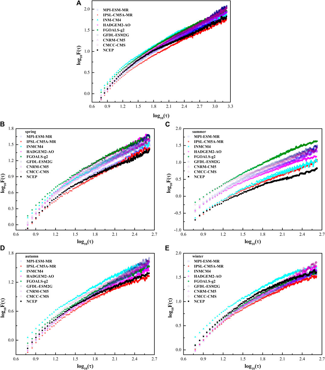
FIGURE 2. The DFA2 results of SAT from NCEP and CMIP5 models at the point of (110°E, 23°N) for (A) year, (B) spring, (C) summer, (D) autumn, and (E) winter.
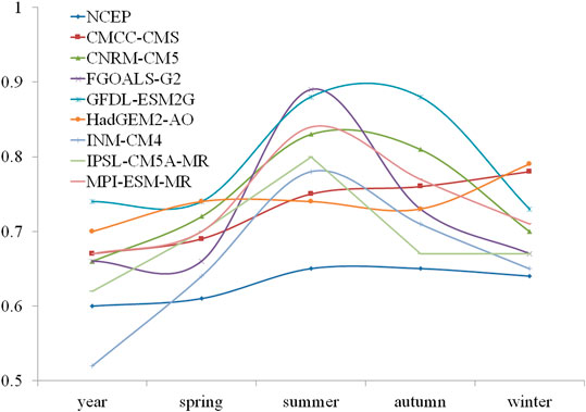
FIGURE 3. The scaling exponents of SAT from NCEP and CMIP5 models at the point of (110°E, 23°N) for year and all four seasons.
Scaling exponent of NCEP SAT throughout the year is less than those of all four seasons at the point, which is also true for most of the model-simulated SAT, except for GFDL-ESM2G (Figure 3). Scaling exponent of NCEP SAT at the point in spring is the smallest among four seasons, while those in summer and autumn are much bigger. The seasonal variations of scaling exponents of most model-simulated SAT are similar to that of NCEP SAT, except for HadGEM2-AO and CMCC-CMS. In general, the difference between the scaling exponent of model-simulated SAT and NCEP data is bigger in summer than that in other seasons.
Figure 4 shows box charts of scaling exponents of NCEP SAT and the biases of scaling exponents of model-simulated SAT on global continents for year and four seasons. The boxes indicate the interquartile distribution (range between the 25th and 75th quantiles). The hollow marked within the boxes show the median, and the short horizontal lines outside the boxes indicate the total inter-model range. The whiskers show the 5% and 95% ranking values. The scaling exponents of SAT throughout the year range from 0.56 to 1.1, and the median value is 0.69 (Figure 4A). Scaling exponents in four seasons vary from 0.52 to 1.14. The median value of the scaling exponents in winter is 0.77, which is bigger than those in other seasons. The median values of the scaling exponent’s biases of SAT throughout the year for CNRM-CM5, GFDL-ESM2G, HadGEM2-AO are close to zero (Figure 4B). The scaling exponents of SAT simulated by FGOALS-g2 and INM-CM4 in most part of world are less than those of NCEP SAT, which means SAT simulated by these two models have weaker LRCs. The scaling exponents of SAT from CMCC-CMS, IPSL-CM5A-MR and MPI-ESM-MR are much bigger than those of NCEP SAT, which shows stronger LRCs in the most part of global continents.
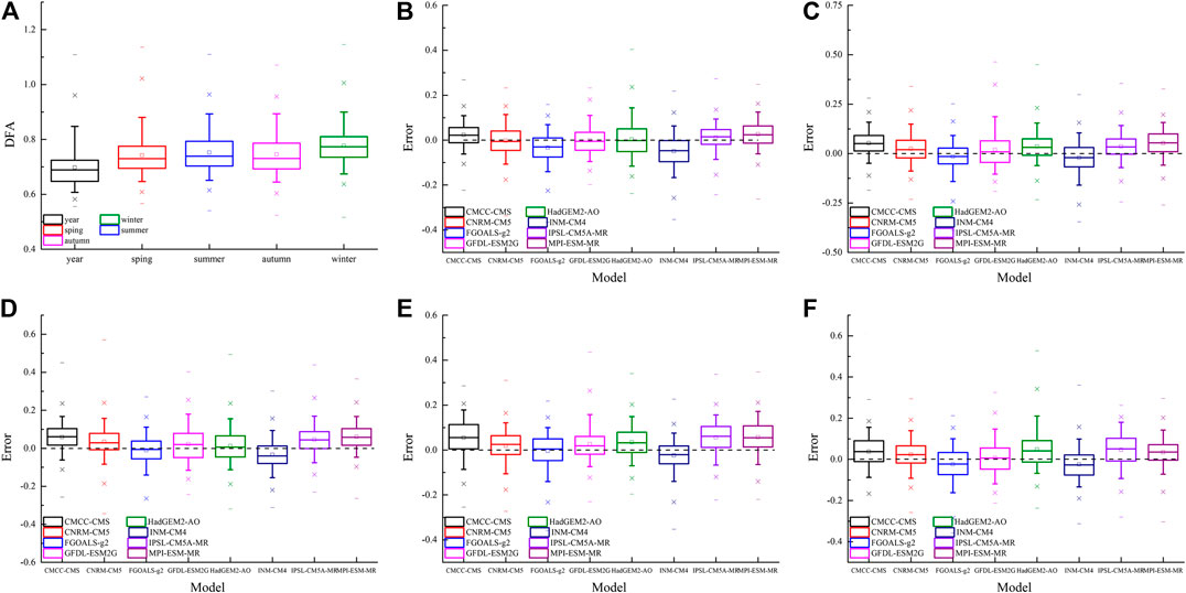
FIGURE 4. Box charts of scaling exponents of NCEP SAT on global continents (A) and the simulation’s errors of LRC of model-simulated SAT for (B) year, (C) spring, (D) summer, (E) autumn, (F) winter.
In boreal spring, the median value of simulation’s errors of GFDL-ESM2G is close to zero, while that of MPI-ESM-MR is 0.06 (Figure 4C). Scaling exponents of SAT simulated by CMCC-CMS, CNRM-CM5, HadGEM2-AO, IPSL-CM5A-MR and MPI-ESM-MR are bigger than those of NCEP SAT in most part of global continents, while those of FGOALS-g2 and INM-CM4 are smaller in most areas of global continents. The median values of the simulation’s error of FGOALS-g2 and HadGEM2-AO are close to zero, while those of CMCC-CMS and IPSL-CM5A-MR are up to 0.06 in boreal summer (Figure 4D). The scaling exponents of SAT simulated by INM-CM4 are smaller than those of NCEP SAT in most part of global continents. In boreal autumn, the median value of the simulation’s errors of LRC in FGOALS-g2 is close to zero, however, the mean value of simulation’s error in IPSL-CM5A-MR is up to 0.07 which is the biggest in all the models (Figure 4E). The scaling exponents of SAT simulated by INM-CM4 are less than those of NCEP SAT in most part of global continent, while the scaling exponents of other models are bigger. The median value of the simulation’s error of LRC of FGOALS-g2 is the smallest, while those of HadGEM2-AO and IPSL-CM5A-MR are bigger than 0.04 in boreal winter (Figure 4F). The scaling exponents of SAT simulated by INM-CM4 are smaller than those of NCEP SAT in most part of global continents, while those of other six models except FGOALS-g2 are much bigger, especially for CMCC-CMS, IPSL-CM5A-MR and MPI-ESM-MR.
The Zonal Distribution Characteristics of Global LRC of SAT
Scaling exponents of NCEP SAT are larger in the tropics than those in middle and high latitude, which shows pronounced latitude dependence (Figure 5A). The zonal mean scaling exponents decrease from equator to middle latitude rapidly. The zonal mean scaling exponents range from 0.7 to 1.0 in tropical areas. From middle latitude to high latitude, the decrement of zonal mean LRC is relatively small. Although the zonal mean of scaling exponents of SAT simulated by 8 CMIP5 models show similar distribution characteristics, there is a great difference among the models. The zonal mean scaling exponents of the model-simulated SAT are close to those of NCEP SAT in the tropics except INM-CM4 and FGOALS-g2. In middle and high latitudes, most of the zonal mean model-simulated scaling exponents are close to those of NCEP SAT except that of HadGEM2-AO. The correlations of zonal mean scaling exponents of model-simulated SAT and those of NCEP SAT all exceed 0.65, which are significant at a significance level of 0.05. The maximum correlation coefficient is 0.89 for CMCC-CMS, while the minimum is 0.66 for MPI-ESM-MR (Table 4).
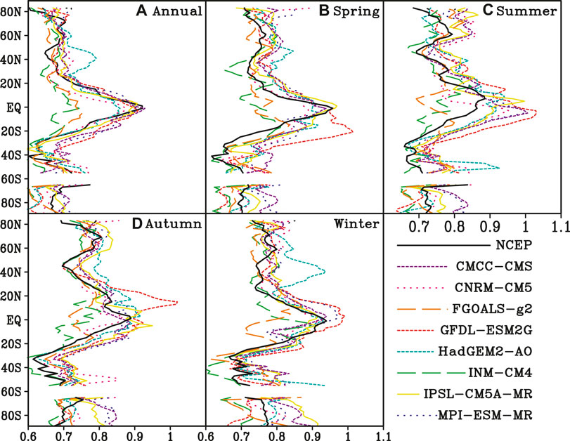
FIGURE 5. Zonal distribution of scaling exponents of NCEP and the 8 model-simulated SAT throughout (A) whole year; (B) spring; (C) summer; (D)autumn; (E) winter.
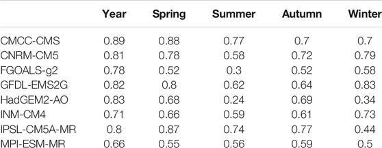
TABLE 4. Correlation coefficients between zonal mean scaling exponents of NCEP and the model-simulated SAT.
In boreal spring, the zonal mean scaling exponent of NCEP SAT is close to 1 at the equator (Figure 5B). It means that NCEP SAT has strong LRC at the equator, and SAT in this area is unstable and very sensitive to small external disturbances. In other words, small disturbances in this area can propagate to other regions through the inner interaction of atmospheric system. From extratropical areas to high latitudes in the northern hemisphere, the zonal mean scaling exponents increase first and then decrease, and the maximum value is about 0.8 near 60°N. In the southern hemisphere, the zonal mean scaling exponents decrease to 0.6 at 40°S, and then increase to about 0.7 in the high latitude. The zonal mean scaling exponents of INM-CM4 and FGOAL-g2 in the tropics are much smaller than those of NCEP SAT, while those of GFDL-ESM2G in the southern tropics are much bigger than those of NCEP SAT. Most of the zonal mean scaling exponents of the model-simulated SAT are bigger than those of NCEP SAT in the high latitudes. The maximum correlation coefficient between zonal mean scaling exponents of the model-simulated SAT and those of NCEP SAT is 0.88 for CMCC-CMS, while the minimum is 0.52 for FGOALS-g2.
In boreal summer, the zonal mean scaling exponents of NCEP SAT are bigger in the northern hemisphere than those in most of the southern hemisphere, and the maximum value is located at about 10°N (Figure 5C). In the northern hemisphere, there are two sub-peak values at 30°N and 60°N, respectively, while the minimum value is about 0.7 at 40°N. In the southern hemisphere, the zonal mean scaling exponents decrease from tropics to the middle-latitude and reach the minimum near 30°S, and then increase in the high latitudes. The differences between zonal mean scaling exponents of NCEP and the model-simulated SAT are bigger in the tropics than those in other areas. The correlation between the zonal mean scaling exponents of NCEP and the model-simulated SAT in summer is significantly reduced compared with that in spring. The maximum correlation coefficient is 0.77 for CMCC-CMS, while the minimum is only 0.24 for HadGEM2-AO.
In boreal autumn, the peak value of zonal mean scaling exponent is close to 0.9 near the equator, and then the zonal mean scaling exponent decreases to about 0.7 near the 40°N and 0.6 near 35°S (Figure 5D). Compared with the zonal mean scaling exponents of NCEP SAT, both INM-CM4 and FGOALS-g2 underestimated LRCs in the tropics, while GFDL-ESM2G significantly overestimates LRCs in northern tropics. The correlations between the zonal mean scaling exponents of the model-simulated SAT and the NCEP data all exceed 0.5. The maximum correlation coefficient is 0.77 for IPSL-CM5A-MR, while the minimum is 0.52 for FGOALS-g2.
In boreal winter, the maximum zonal mean scaling exponent of NCEP SAT is greater than 0.9 near the equator. The zonal mean scaling exponents in the middle and high latitudes of the northern hemisphere are between 0.7 and 0.8, which have smaller variations than those in the southern hemisphere. The zonal mean scaling exponents reach the minimum near 40°S, and then increase to 0.8 in the Antarctic region (Figure 5E). In the tropics, the zonal mean scaling exponents of SAT simulated by FGOALS-g2 are obviously smaller than those of NCEP SAT, while those of GFDL-ESM2G are larger. The zonal mean scaling exponents of HadGEM2-AO are larger than those of NCEP SAT in the middle and high latitudes in the northern hemisphere. The differences between the zonal mean scaling exponents of NCEP and most of the model-simulated SAT are relatively larger in the middle and high latitudes of the southern hemisphere than those in other areas. The correlation between zonal mean scaling exponents of the model-simulated SAT and those of NCEP SAT has large variations with the maximum coefficient of 0.84 for GFDL-ESM2G and the minimum of 0.34 for HadGEM2-AO.
In general, the zonal mean scaling exponents of NCEP SAT are big in the tropics and small in the middle and high latitudes, which also exhibit obvious seasonal variation. The zonal distributions of scaling exponents in boreal spring are similar with those in winter, with bigger scaling exponents in the northern hemisphere than the southern hemisphere. The zonal distributions of scaling exponents in summer and autumn are also similar, with two sub-peaks in the northern hemisphere and increasing trend from middle to high latitudes. In the tropics, the zonal mean scaling exponents of INM-CM4 and FGOALS-g2 are both smaller than those of NCEP SAT, while those of GFDL-ESM2G are bigger. In a word, the performance of CMIP5 models to LRC has seasonal variation.
Evaluation of Performance of the Model-Simulated SAT Based on the Spatial Distribution Characteristics of LRC
NCEP SAT has LRC characteristics in most parts of the global continents. The scaling exponents are bigger in the tropics than those in other regions. Scaling exponents range from 0.75 to 0.95 in Central Africa and South Asia, and exceed 0.95 in North South America (Figure 6A). Compared with the scaling exponents of NCEP SAT, more than 60% of the DFA differences of CMCC-CMS, CNRM-CM5, GFDL-ESM2G, IPSL-CM5A-MR and MPI-ESM-MR are not significant at a significance level of 0.05, which means the performance is good in most of global continents. The performance of IPSL-CM5A-MR is the best among all models with 69.1% of global continents where the simulation’s errors are not significant, especially in the northern part of Eurasia, South America and Australia (Figure 6H). CMCC-CMS, CNRM-CM5, HadGEM2-AO and MPI-ESM-MR overestimate the LRC of SAT in most parts of the tropics (Figures 6B,C,F,I), while both FGOALS-g2 and INM-CM4 underestimate the LRC of SAT in most parts of the global continents (Figures 6D,G). The performance of INM-CM4, FGOALS-g2 and HadGEM2-AO is relatively poor.
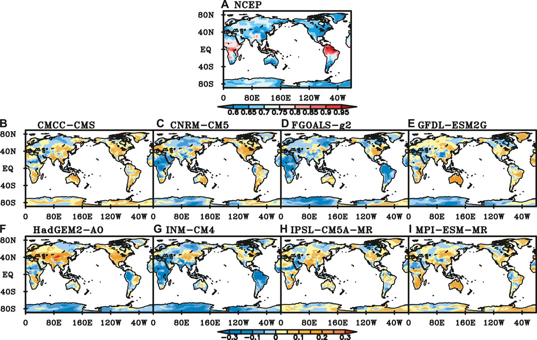
FIGURE 6. Scaling exponents of NCEP SAT (A) and difference between NCEP and those of SAT simulated by (B) CMCC-CMS, (C) CNRM-CM5, (D) FGOALS-g2, (E) GFDL-ESM2G, (F) HadGEM-AO, (G) INM-CM4, (H) IPSL-CM5A-MR, (I) MPI-ESM-MR. (Black dot represents the difference is significant at a significance level of 0.05).
To explore the performance of individual models in different regions, we calculated the percentage of grids with insignificant errors in each region. If the percentage of good performance grids in one region exceeds 50%, it’s considered that the model performance is good in this region. Based on this, the performance of most CMIP5 models is good in SIB, NEU, CAS and GRL regions, while relatively poor in EAS, SAS, SEA and CNA. Both IPSL-CM5A-MR and FGOALS-g2 have five regions with the best performance among the 8 CMIP5 models. However, HadGEM2-AO has six regions of the poorest performance among the 8 models.
In boreal spring, the scaling exponents of NCEP SAT in most parts of the global continents are greater than 0.6. The scaling exponents are between 0.6 and 0.7 in eastern China, northern Africa, northwestern North America, South America, eastern Australia and Antarctic, and exceed 0.9 in northern South America (Figure 7A). Compared with the scaling exponents of NCEP data, those of model-simulated SAT are smaller in northern South America, and those of SAT from CNRM-CM5, FGOALS-g2 and INM-CM4 are smaller in the tropics (Figures 7B,D,G). The percentage of insignificant simulation’s errors of LRC is less than 60% for CMCC-CMS, GFDL-ESM2G and MPI-ESM-MR. SAT of GFDL-ESM2G has stronger LRC than NCEP SAT in Australia, southern Africa and southern South America (Figure 7E), while those of GFDL-ESM2G and INM-CM4 have weaker LRC in Antarctica (Figures 7E,G). The performance of FGOALS-g2 is the best with 71.9% of global continents where the simulation’s errors of LRC are insignificant, while the performance of MPI-ESM-MR is the poorest among all eight models with 50.3% of global continents.
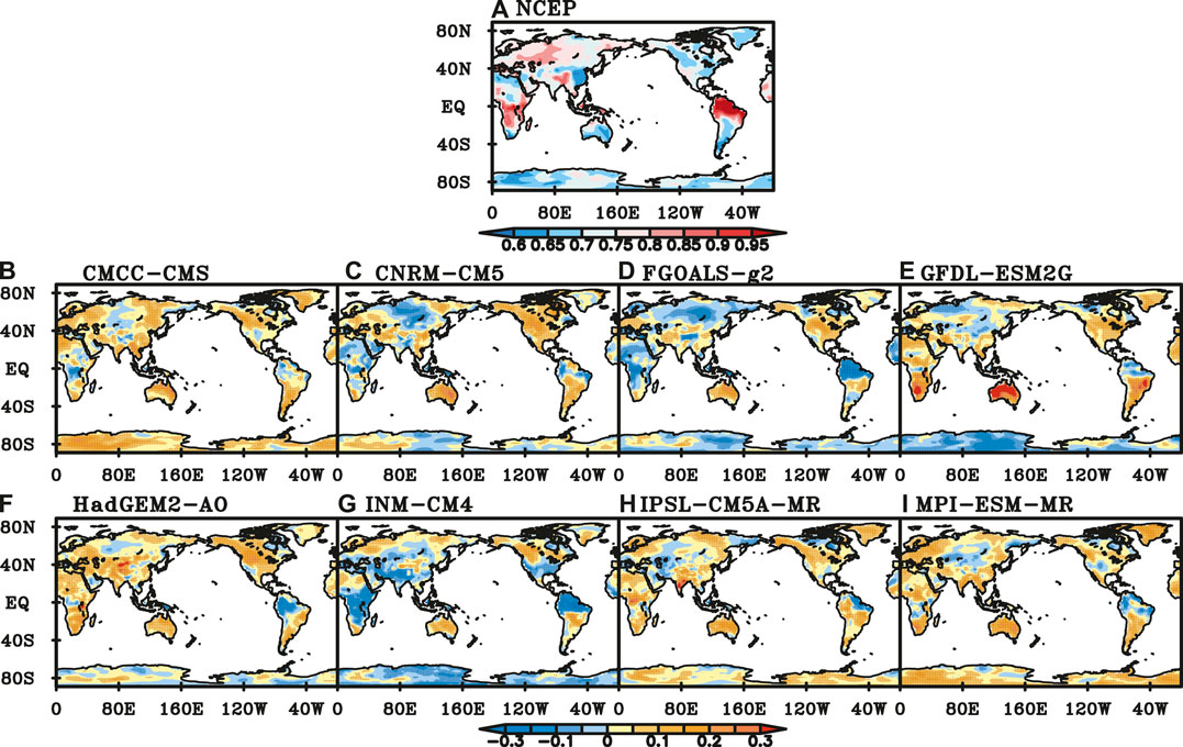
FIGURE 7. Scaling exponents of NCEP SAT (A) and difference between NCEP and those of SAT simulated by (B) CMCC-CMS, (C) CNRM-CM5, (D) FGOALS-g2, (E) GFDL-ESM2G, (F) HadGEM-AO, (G) INM-CM4, (H) IPSL-CM5A-MR, (I) MPI-ESM-MR in spring. (Black dot represents the difference is significant at a significance level of 0.05).
The performance of CMIP5 models is good in SIB, CAS and TIB, while poor in WAF, AUS and SEA. The percentage of good performance grids of 8 CMIP5 models exceeds 60% in SIB, while less than 50% in AUS. INM-CM4 has five regions of the best performance among 8 models. Followed by FGOALS-g2 and GFDL-ESM2G, both of them have four regions. However, CNRM-CM5 has six regions of the poorest performance, especially in CAN. Next, both GFDL-ESM2G and MPI-ESM-MR have four regions of the worst performance.
In boreal summer, the scaling exponents of NCEP SAT are bigger than those in spring in most of global continents except in the middle of Eurasia and northern South America. The scaling exponents in the tropical region are greater than 0.8 (Figure 8A). Compared with the scaling exponents of NCEP SAT, CNRM-CM5, FGOALS-g2 and INM-CM4 have relatively better capabilities in simulating SAT than the other five models, with more than 60% of global continents where the simulation’s errors of LRC are insignificant. The LRCs of SAT from CMCC-CMS, IPSL-CM5A-MR and MPI-ESM-MR are weaker than those of NCEP SAT in local areas of North American (Figures 8B,H,I). Scaling exponents of FGOALS-g2 are bigger in eastern Eurasia, Australia and Greenland (Figure 8D). GFDL-ESM2G and HadGEM2-AO have smaller scaling exponents in the high latitudes (Figures 8E,F). INM-CM4 has smaller scaling exponents in most parts of the global continents (Figure 8G).
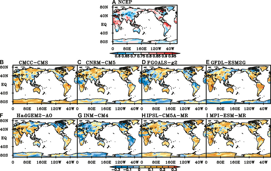
FIGURE 8. Scaling exponents of NCEP SAT (A) and difference between NCEP and those of SAT simulated by (B) CMCC-CMS, (C) CNRM-CM5, (D) FGOALS-g2, (E) GFDL-ESM2G, (F) HadGEM-AO, (G) INM-CM4, (H) IPSL-CM5A-MR, (I) MPI-ESM-MR in summer. (Black dot represents the difference is significant at a significance level of 0.05).
The percentage of good performance girds in NEU exceeds 62% for most models except INM-CM4. In EAF, GRL, SAF, MED and SEA, the performance of most models is poor. In EAF and GRL, the percentage of good performance grids for all models is less than 50%. FGOALS-g2 has seven best-performance regions, while GFDL-ESM2G has seven regions of the poorest performance.
In boreal autumn, the distributions of scaling exponents of NCEP SAT are similar to those in summer, with smaller values in most part of Eurasia than those in other regions. The scaling exponents of NCEP SAT are generally between 0.6 and 0.7 in the middle and high latitudes of the southern hemisphere, central and southern North America, and eastern Asia, while greater than 0.85 in northern South America, central and northern Africa, South Asia and North America (Figure 9A). Compared with the scaling exponents of NCEP SAT, those of CMCC-CMS, IPSL-CM5A-MR and MPI-ESM-MR are bigger in the southern hemisphere and North America, while smaller in northern Africa and northeastern North America (Figures 9B,H,I). The scaling exponents of CNRM-CM5 are close to those of NCEP in most parts of the global continents, except in the northern and southern parts of Eurasia, northern Africa, northeastern North America, and northern South America (Figure 9C). Scaling exponents of FGOALS-g2 are smaller in northern Eurasia, central and North Africa, North America, northeastern North America, and most parts of South America (Figure 9D). LRCs of DTA simulated by GFDL-ESM2G are stronger in parts of Africa, South Asia, eastern Australia, South America and North America, while weaker in the middle of Eurasia, the northeastern part of North America (Figure 9E). Scaling exponents of HadGEM2-AO are close to those of NCEP SAT in most regions of the southern hemisphere, while greater in most part of the northern hemisphere (Figure 9F). INM-CM4 has weaker LRC in parts of Africa, northern South America, eastern Australia, northern Eurasia, northeastern North America, and Antarctica (Figure 9G).
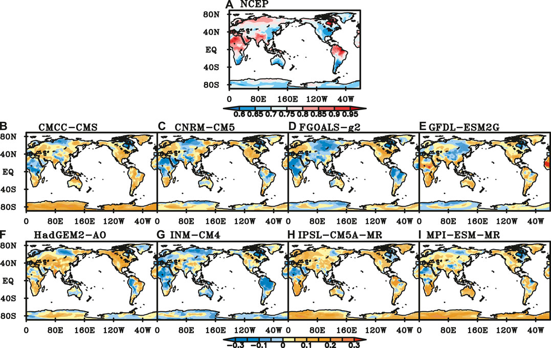
FIGURE 9. Scaling exponents of NCEP SAT (A) and difference between NCEP and those of SAT simulated by (B) CMCC-CMS, (C) CNRM-CM5, (D) FGOALS-g2, (E) GFDL-ESM2G, (F) HadGEM-AO, (G) INM-CM4, (H) IPSL-CM5A-MR, (I) MPI-ESM-MR in autumn. (Black dot represents the difference is significant at a significance level of 0.05).
All the 8 CMIP5 models perform well in SIB. In MED and TIB, most of the models except HadGEM2-AO have good performance. The performance of most models is poor in NSA, MEX, CNA and SAF. In CNA, the percentage of good performance grids for CMCC-CMS, CNRM-CM5, FGOALS-g2 and HadGEM2-AO is less than 10%. INM-CM4 has six regions of the best performance among the 8 models. CMCC-CMS has four regions of the best performance. However, HadGEM2-AO has five regions of the poorest performance, and CMCC-CMS has four regions.
In boreal winter, the distributions of scaling exponents of NCEP SAT are similar to those in spring, with bigger values in Eurasia, northern South American and middle and southern South African than those in other areas. The scaling exponents are between 0.6 and 0.7 only in eastern China, southwestern Australia, south South America and south central North America. In the rest of the global continents, the scaling exponents are generally above 0.75, and exceed 0.9 in North America and Central Africa (Figure 10A).
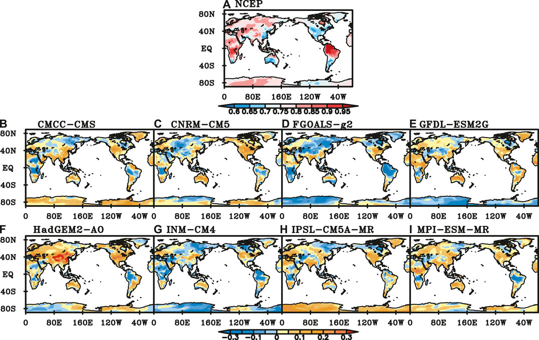
FIGURE 10. Scaling exponents of NCEP SAT (A) and difference between NCEP and those of SAT simulated by (B) CMCC-CMS, (C) CNRM-CM5, (D) FGOALS-g2, (E) GFDL-ESM2G, (F) HadGEM-AO, (G) INM-CM4, (H) IPSL-CM5A-MR, (I) MPI-ESM-MR in winter. (Black dot represents the difference is significant at a significance level of 0.05).
Compared with scaling exponents of NCEP SAT, those of CMCC-CMS, IPSL-CM5A-MR and MPI-ESM-MR are greater in South Eurasia, northern South America, Antarctic, and parts of Australia, while smaller in middle and southern Africa, Greenland, northern South America (Figures 10B,H,I). Those of CNRM-CM5 are smaller in equator, Central Europe, northern South America, while greater in central Australia as well as middle and northern North America (Figure 10C). The scaling exponents of FGOALS-g2 and INM-CM4 are smaller in Greenland, northern South America, southeastern North America, central and southern African and Antarctic, while greater in southern North America, northern Australia (Figures 10D,G). LRCs of SAT simulated by GFDL-ESM2G are stronger in the tropics while weaker in Antarctic, north-eastern North America and central Eurasia (Figure 10E). LRCs of SAT simulated by HadGEM2-AO are weaker in the tropics, while stronger in other areas (Figure 10F). Scaling exponents of INM-CM4 are smaller in most part of the global continents except in the mid-latitude regions (Figure 10G).
All the 8 models perform well in SIB and GRL region. In TIB, most of the models except HadGEM2-AO have good performance. The performance of most models is poor in CNA and SEA. In CAN, all the 8 models have poor performance. CMCC-CMS has the best performance in six regions, and CNRM-CM5 has five best-performance regions. However, HadGEM2-AO has seven regions in which the performance is the poorest. Both CMCC-CMS and CNRM-CM5 have five regions of the poorest performance.
Conclusion
Based on the LRCs of daily average SAT, the performance of 8 CMIP5 models in global continents is quantitatively evaluated using DFA method. The DFA results of NCEP SAT show that the SAT has a long-range correlation in most regions of the global continents. The scaling exponents of NCEP SAT show zonal distribution characteristics, which are bigger in tropics than that in middle and high latitudes. The zonal distribution of SAT from CMCC-CMS is the most similar to that of NCEP data in spring, summer and throughout the year. The zonal distributions of scaling exponents of IPSL-CM5A-MR and GFDL-ESM2G are the most similar to those of NCEP data in autumn and winter,respectively. Compared with the zonal distribution of NCEP SAT, that of FGOALS-g2 has the greatest bias in spring and autumn. HadGEM2-AO has the greatest bias in summer, and HadGEM2-AO has the greatest bias in winter.
Although the performance of models varies in different seasons, there is still something in common. Scaling exponents of SAT simulated by CMCC-CMS, IPSL-CM5A-MR as well as MPI-ESM-MR are smaller in North American while greater in other regions than those of NCEP SAT in all four seasons. This means LRCs of the simulated SAT are stronger than those of NCEP in most areas except North American. Scaling exponents of SAT simulated by FGOALS-g2 and INM-CM4 are less than those of NCEP SAT in most areas, especially in northern South American, most part of African and parts of Eurasia. Scaling exponents of SAT from GFDL-ESM2G are greater in most part of middle latitude of southern hemisphere. Scaling exponents of SAT from CNRM-CM5 and HadGEM2-AO are greater in North American in all four seasons.
The performance of the 8 models also varies in different regions. The scaling exponents of most model-simulated SAT are close to those of NCEP data at middle and high latitudes of the Northern Hemisphere, such as SIB, NEU, GRL and CAS regions, which means the dynamical characteristics of climate systems in these areas are well simulated by the models. However, the DFA errors are big in East Asia and CAN regions. In spring, the performance of most models is good in SIB, CAS and TIB, especially in SIB, but poor in WAF, AUS and SEA. In summer, the performance of most models is good in NEU area, but poor in EAF, SAF, GRL, MED and SEA area. Kumar et al. (2014) showed that some CMIP5 models had warm bias in boreal summer and the performance of the models was poor over EAF, SAF and SEA. In autumn, most models have good performance in SIB, MED and TIB areas, but poor performance in NSA, MEX, CAN and SAF areas. In winter, most models have good performance in SIB, GRL and TIB areas, but poor performance in CAN and SEA areas.
The performance of IPSL-CM5A-MR is the best among the 8 models while that of HadGEM2-AO is the poorest throughout the year. Liu et al. (2014) also pointed out that HadGEM2-AO had poor performance on SAT over China, while INM-CM4 had good performance. The performance of models varies greatly with seasons. FGOALS-g2 has good performance in spring and summer. GFDL-ESM2G has good performance in autumn. CNRM-CM5 and CMCC-CMS has good performance in winter. However, MPI-ESM-MR has the poorest performance in spring. The performance of CMCC-CMS and GFDL-EMS2G is poor in summer. HadGEM2-AO has poor performance in autumn and winter.
Generally speaking, the comparison of individual models for certain regions and seasons reveals that the most of models can reasonably simulate the dynamical characteristics of climate systems in most regions, while there are inter-model differences in various regions and seasons. These differences maybe induced by the processes of climate models, which needs a further examination in the future. Therefore, appropriate models should be selected according to the research regions and seasons.
Data Availability Statement
The original contributions presented in the study are included in the article/Supplementary Material, further inquiries can be directed to the corresponding author.
Author Contributions
SZ analyzed the data and wrote the manuscript. WH revised the manuscript. TD, JZ, XX, YM, SW, and YJ offered the suggestion.
Funding
This research was jointly supported by National Natural Science Foundation of China (Grant Nos. 41875120, 41775092, 41975086, 42075051 and 41605069), and the Fundamental Research Funds for the Central Universities (Grant Nos. 20lgzd06).
Conflict of Interest
The authors declare that the research was conducted in the absence of any commercial or financial relationships that could be construed as a potential conflict of interest.
Supplementary Material
The Supplementary Material for this article can be found online at: https://www.frontiersin.org/articles/10.3389/fenvs.2021.628999/full#supplementary-material.
References
Blender, R., and Fraedrich, K. (2003). Long time memory in global warming simulations. Geophys. Res. Lett. 30, 1769–1722. doi:10.1029/2003GL017666
Bunde, A., Eichner, J. F., Kantelhardt, J. W., and Havlin, S. (2005). Long-term memory: a natural mechanism for the clustering of extreme events and anomalous residual times in climate records. Phys. Rev. Lett. 94, 048701. doi:10.1103/PhysRevLett.94.048701
Bunde, A., and Havlin, S. (2002). Power-law persistence in the atmosphere and in the oceans. Phys. Stat. Mech. Appl. 314, 15–24. doi:10.1016/s0378-4371(02)01050-6
Chan, D., and Wu, Q. (2015). Attributing observed SST trends and subcontinental land warming to anthropogenic forcing during 1979-2005. J. Clim. 28, 3152–3170. doi:10.1175/JCLI-D-14-00253.1
Eichner, J. F., Koscielny-Bunde, E., Bunde, A., Havlin, S., and Schellnhuber, H. J. (2003). Power-law persistence and trends in the atmosphere: a detailed study of long temperature records. Phys. Rev. E - Stat. Nonlinear Soft Matter Phys. 68, 046133. doi:10.1103/PhysRevE.68.046133
Elguindi, N., Grundstein, A., Bernardes, S., Turuncoglu, U., and Feddema, J. (2014). Assessment of CMIP5 global model simulations and climate change projections for the 21 st century using a modified Thornthwaite climate classification. Climatic Change 122, 523–538. doi:10.1007/s10584-013-1020-0
Flato, G., Marotzke, J., Abiodun, B., and Braconnot, P. (2013). Evaluation of climate models. Climate change 2013: the physical science basis. Contribution of working group I to the fifth assessment report of the intergovernmental panel on climate change. Cambridge, United Kingdom: Cambridge University Press, 746–866.
Fu, Z., Shi, L., Xie, F., and Piao, L. (2016b). Nonlinear features of northern annular mode variability. Phys. Stat. Mech. Appl. 449, 390–394. doi:10.1016/j.physa.2016.01.014
Fu, Z., Xie, F., Yuan, N., and Piao, L. (2016a). Impact of previous one-step variation in positively long-range correlated processes. Theor. Appl. Climatol. 124, 339–347. doi:10.1007/s00704-015-1419-9
Gan, Z., Yan, Y., and Qi, Y. (2007). Scaling analysis of the sea surface temperature anomaly in the south China sea. J. Atmos. Ocean. Technol. 24, 681–687. doi:10.1175/JTECH1981.1
Giorgi, F. (2002). Variability and trends of sub-continental scale surface climate in the twentieth century. Part I: observations. Clim. Dynam. 18, 675–691. doi:10.1007/s00382-001-0204-x
Govindan, R. B., Vyushin, D., Bunde, A., Brenner, S., Havlin, S., and Schellnhuber, H. J. (2004). Global climate models violate scaling of the observed atmospheric variabilit. Phys. Rev. Lett. 92, 028501. doi:10.1103/PhysRevLett.92.159803
He, W.-P., and Zhao, S.-S. (2018). Assessment of the quality of NCEP-2 and CFSR reanalysis daily temperature in China based on long-range correlation. Clim. Dynam. 50, 493–505. doi:10.1007/s00382-017-3622-0
He, W., Zhao, S., Liu, Q., Jiang, Y., and Deng, B. (2016). Long-range correlation in the drought and flood index from 1470 to 2000 in eastern China. Int. J. Climatol. 36, 1676–1685. doi:10.1002/joc.4450
Jiang, D., Tian, Z., and Lang, X. (2016). Reliability of climate models for China through the IPCC third to fifth assessment reports. Int. J. Climatol. 36, 1114–1133. doi:10.1002/joc.4406
Jiang, L., Li, N., Fu, Z., and Zhang, J. (2015). Long-range correlation behaviors for the 0-cm averages ground surface temperature and average air temperature over China. Theor. Appl. Climatol. 119, 25–31. doi:10.1007/s00704-013-1080-0
Josey, S. A. (2001). A comparison of ECMWF, NCEP/NCAR, and SOC surface heat fluxes with moored buoy measurements in the subduction region of the Northeast Atlantic. J. Clim. 14, 1780–1789. doi:10.1175/1520-0442(2001)014<1780:acoenn>2.0.co;2
Kalnay, E., Kanamitsu, M., Kistler, R., Collins, W., Deaven, D., Gandin, L., et al. (1996). The NCEP/NCAR 40-year reanalysis project, Bull. Am. Meteorol. Soc. 77, 437–471. doi:10.1175/1520-0477(1996)077<0437:TNYRP>2.0.CO;2
Kanamitsu, M., Ebisuzaki, W., WoollenYang, J. S. K., Yang, S.-K., Hnilo, J. J., Fiorino, M., et al. (2002). NCEP-DOE AMIP-II reanalysis (R-2). Bull. Am. Meteorol. Soc. 83, 1631–1644. doi:10.1175/Bams-83-11-1631
Kantelhardt, J. W., Koscielny-Bunde, E., Rybski, D., Braun, P., Bunde, A., and Havlin, S. (2006). Long-term persistence and multifractality of precipitation and river runoff records. J. Geophys. Res. 111, D01106. doi:10.1029/2005JD005881
Kharin, V. V., Zwiers, F. W., Zhang, X., and Wehner, M. (2013). Changes in temperature and precipitation extremes in the CMIP5 ensemble. Climatic Change. 119, 345–357. doi:10.1007/s10584-013-0705-8
Király, A., and Jánosi, I. M. (2005). Detrended fluctuation analysis of daily temperature records: geographic dependence over Australia. Meteorol. Atmos. Phys. 88, 119–128. doi:10.1007/s00703-004-0078-7
Koscielny-Bunde, E., Bunde, A., Havlin, S., and Goldreich, Y. (1996). Analysis of daily temperature fluctuations. Phys. Stat. Mech. Appl. 231, 393–396. doi:10.1016/0378-4371(96)00187-210.1016/0378-4371(96)00187-2
Koscielny-Bunde, E., Roman, H. E., Bunde, A., Havlin, S., and Schellnhuber, H. J. (1998). Long-range power-law correlations in local daily temperature fluctuation. Phil. Mag. B 77, 1331–1340. doi:10.1080/13642819808205026
Kumar, D., Kodar, E., and Ganguly, A. R. (2014). Regional and seasonal intercomparison of CMIP3 and CMIP5 climate model ensembles for temperature and precipitation. Clim. Dynam. 43, 2491–2518. doi:10.1007/s00382-014-2070-3
Kumar, S., Merwade, V., Kinter, J. L., and Niyogi, D. (2013). Evaluation of temperature and precipitation trends and long-term persistence in CMIP5 twentieth-century climate simulations. J. Clim. 26, 4168–4185. doi:10.1175/JCLI-D-12-00259.1
Li, Q., Zhang, L., Xu, W., Zhou, T., Wang, J., Zhai, P., et al. (2017). Comparisons of time series of annual mean surface air temperature for China since the 1900s: observations, model simulations, and extended reanalysis. Bull. Am. Meteorol. Soc. 98, 699–711. doi:10.1175/BAMS-D-16-0092.1
Liu, Y., Feng, J., and Ma, Z. (2014). An analysis of historical and future temperature fluctuations over China based on CMIP5 simulations. Adv. Atmos. Sci. 31, 457–467. doi:10.1007/s00376-013-3093-0
Ma, L., Zhang, T., Li, Q., Frauenfeld, O. W., and Qin, D. (2008). Evaluation of ERA-40, NCEP-1, and NCEP-2 reanalysis air temperature with ground-based measurements in China. J. Geophys. Res. 113, D15115. doi:10.1029/2008jd010981
Marques, C. A. F., Rocha, A., and Corte-Real, J. (2010). Comparative energetics of ERA-40, JRA-25 and NCEP-R2 reanalysis, in the wave number domain. Dynam. Atmos. Oceans 50, 375–399. doi:10.1016/j.dynatmoce.2010.03.003
Mooney, P. A., Mulligan, F. J., and Fealy, R. (2011). Comparison of ERA-40, ERA-interim and NCEP/NCAR reanalysis data with observed surface air temperature over Ireland. Int. J. Climatol. 31, 545–557. doi:10.1002/joc.2098
Mueller, T. G., Pusuluri, N. B., Mathias, K. K., Cornelius, P. L., Barnhisel, R. I., and Shearer, S. A. (2004). Map quality for ordinary kriging and inverse distance weighted interpolation. Soil Sci. Soc. Am. J. 68, 2042–2047. doi:10.2136/sssaj2004.2042
Peng, C. K., Havlin, S., Schwartz, M., and Stanley, H. E. (1991). Directed-polymer and ballistic-deposition growth with correlated noise. Phys. Rev. A. 44, R2239–R2242. doi:10.1103/PhysRevA.44.R2239
Peng, C. K., Buldyrev, S. V., Havlin, S., Simons, M., Stanley, H. E., and Goldberger, A. L. (1994). Mosaic organization of DNA nucleotides. Phys. Rev. E. 49, 1685–1689. doi:10.1103/PhysRevE.49.1685
Phillips, T. J., and Gleckler, P. J. (2006). Evaluation of continental precipitation in 20th century climate simulations: the utility of multimodel statistics. Water Resour. Res. 42, W03202. doi:10.1029/2005WR004313
Poccard, I., Janicot, S., and Camberlin, P. (2000). Comparison of rainfall structure between NCEP/NCAR reanalysis and observed data over tropical Africa. Clim. Dynam. 16, 897–915. doi:10.1007/s003820000087
Rybski, D., Bunde, A., and von Storch, H. (2008). Long-term persistence in 1000-year simulated temperature records. J. Geophys. Res. 113, D02106. doi:10.1029/2007JD008568
Sillmann, J., Kharin, V. V., Zhang, X., Zwiers, F. W., and Bronaugh, D. (2013). Climate extremes indices in the CMIP5 multimodel ensemble: Part 1. Model evaluation in the present climate. J. Geophys. Res. Atmos. 118, 1716–1733. doi:10.1002/jgrd.50203
Sillmann, J., Kharin, V. V., Zwiers, F. W., Zhang, X., Bronaugh, D., and Donat, M. G. (2014). Evaluating model-simulated variability in temperature extremes using modified percentile indices. Int. J. Climatol. 34, 3304–3311. doi:10.1002/joc.3899
Talkner, P., and Weber, R. O. (2000). Power spectrum and detrended fluctuation analysis: application to daily temperatures. Phys. Rev. E. 62, 150–160. doi:10.1103/PhysRevE.62.150
Taylor, K. E., Stouffer, R. J., and Meehl, G. A. (2012). An overview of CMIP5 and the experiment design. Bull. Am. Meteorol. Soc. 93, 485–498. doi:10.1175/BAMS-D-11-00094.1
Watterson, I. G., Bathols, J., and Heady, C. (2014). What influences the skill of climate models over the continents?. Bull. Am. Meteorol. Soc. 95, 689–700. doi:10.1175/BAMS-D-12-00136.1
Weber, R. O., and Talkner, P. (2001). Spectra and correlations of climate data from days to decades. J. Geophys. Res. 106, 20131–20144. doi:10.1029/2001JD000548
Yin, L., Fu, R., Shevliakova, E., and Dickinson, R. E. (2013). How well can CMIP5 simulate precipitation and its controlling processes over tropical south America?. Clim. Dynam. 41, 3127–3143. doi:10.1007/s00382-012-1582-y
Yuan, N., Ding, M., Huang, Y., Fu, Z., Xoplaki, E., and Luterbacher, J. (2015). On the long-term climate memory in the surface air temperature records over Antarctica: a nonnegligible factor for trend evaluation. J. Clim. 28, 5922–5934. doi:10.1175/JCLI-D-14-00733.1
Zhao, S., He, W., and Jiang, Y. (2017). Evaluation of NCEP-2 and CFSR reanalysis seasonal temperature data in China using detrended fluctuation analysis. Int. J. Climatol. 38, 252–263. doi:10.1002/joc.5173
Zhao, S. S., and He, W. P. (2014). Performance evaluation of Chinese air temperature simulated by Beijing Climate Center Climate System Model on the basis of the long-range correlation [in Chinese]. Acta Phys. Sin. 63, 209201. doi:10.7498/aps.63.209201
Zhao, S. S., and He, W. P. (2015). Performance evaluation of the simulated daily average temperature series in four seasons in China by Beijing Climate system model. Acta Phys. Sin. 64, 049201 [In Chinese, with English summary]. doi:10.7498/aps.64.049201
Keywords: detrended fluctuation analysis, long-range correlation, CMIP5, model intercomparision, surface air temperature
Citation: Zhao S, He W, Dong T, Zhou J, Xie X, Mei Y, Wan S and Jiang Y (2021) Evaluation of the Performance of CMIP5 Models to Simulate Land Surface Air Temperature Based on Long-Range Correlation. Front. Environ. Sci. 9:628999. doi: 10.3389/fenvs.2021.628999
Received: 13 November 2020; Accepted: 07 January 2021;
Published: 16 February 2021.
Edited by:
Boyin Huang, National Oceanic and Atmospheric Administration, United StatesCopyright © 2021 Zhao, He, Dong, Zhou, Xie, Mei, Wan and Jiang. This is an open-access article distributed under the terms of the Creative Commons Attribution License (CC BY). The use, distribution or reproduction in other forums is permitted, provided the original author(s) and the copyright owner(s) are credited and that the original publication in this journal is cited, in accordance with accepted academic practice. No use, distribution or reproduction is permitted which does not comply with these terms.
*Correspondence: Wenping He, d2VucGluZ19oZUAxNjMuY29t