Seasonal Variation in Chemical Composition of Size-Segregated Aerosols Over the Northeastern Arabian Sea

Water-soluble species constitute a significant fraction (up to 60–70%) of the total aerosol loading in the marine atmospheric boundary layer (MABL). The “indirect” effects, that is, climate forcing due to modification of cloud properties depend on the water-soluble composition of aerosols. Thus, the characterization of aerosols over the MABL is of greater relevance. Here, we present 1-year long aerosol chemical composition data of PM₁₀ and PM_2.5 at a costal location in the northeastern Arabian Sea (Goa; 15.45°N, 73.20°E, 56 m above the sea level). Average water-soluble ionic concentration (sum of anion and cation) is highest (25.5 ± 6.9 and 19.6 ± 5.8 μg·m⁻³ for PM₁₀ and PM_2.5, respectively) during winter season and lowest during post-monsoon (17.3 ± 9.1 and 14.4 ± 8.1 μg·m⁻³ for PM₁₀ and PM_2.5, respectively). Among water-soluble ionic spices, SO₄^2- ion was found to be dominant species in anions and NH₄⁺ is dominant in cations, for both PM₁₀ and PM_2.5 during all the seasons. These observations clearly hint to the contribution from anthropogenic emission and significant secondary inorganic species formation. Sea-salt (calculated based on Na⁺ and Cl⁻) concentration shows significant temporal variability with highest contribution during summer seasons in both fractions. Sea-salt corrected Ca²⁺, an indicator of mineral dust is found mostly during summer months, particularly in PM₁₀ samples, indicates contribution from mineral dust emissions from arid/semiarid regions located in the north/northwestern India and southwest Asia. These observations are corroborated with back-trajectory analyses, wherein air parcels were found to derive from the desert area in summer and Indo-Gangetic Plains (a hot spot for anthropogenic emissions) during winter. In addition, we also observe the presence of nss-K⁺ (sea-salt corrected), for PM_2.5, particularly during winter months, indicating influence of biomass burning emissions. The impact on aerosol chemistry is further assessed based on chloride depletion. Chloride depletion is observed very significant during post-monsoon months (October and November), wherein more than 80 up to 100% depletion is found, mediated by excess sulfates highlighting the role of secondary species in atmospheric chemistry. Regional scale characterization of atmospheric aerosols is important for their better parameterization in chemical transport model and estimation of radiative forcing.

Introduction

Atmospheric aerosols, derived from continental regions, undergo long-range transport and supply significant amount of nutrients as well as toxicants to remote and coastal oceanic region (Jickells et al., 2005; Paytan et al., 2009; Kumar et al., 2010; Jordi et al., 2012; Baker et al., 2013; Srinivas and Sarin, 2013a; Powell et al., 2015; Kumar et al., 2020). In addition, aerosols emitted from marine region (mainly sea salt) can impact on the chemical composition of aerosols over the continent and, thus, play a vital role in atmospheric chemistry (Quinn et al., 2004; Keene et al., 2007; Kumar and Sarin, 2009; Sarin et al., 2011). The availability (and lability) of nutrients/toxicants significantly depend on the ambient atmospheric chemistry (Baker and Croot, 2010; Kumar and Sarin, 2010a), which eventually undergo dry (Arimoto et al., 2003; Srinivas and Sarin, 2013a; Baker et al., 2017) as well as wet (Measures and Vink, 1999; Chance et al., 2015; Powell et al., 2015) deposition. Post deposition, they can modulate surface water biogeochemical processes (Mahowald et al., 2005; Guieu et al., 2019; Anderson, 2020) which have impact on carbon cycling and eventually on Earth’s climate (Ramanathan et al., 2001; Barnett et al., 2005; Rana et al., 2019).

The lifetime of atmospheric aerosols ranges from few hours to several days, and thus, they display large temporal variability (Pöschl, 2005). In addition, varying emission intensity and their source region also contribute to their temporal as well as spatial variability. The impact of aerosols can be assessed more quantitatively by having information on their chemical composition as well as their emission sources. For example, aerosols with more acidic composition have more processed labile Fe content (Baker and Croot, 2010; Kumar et al., 2010) and can impact significantly on primary productivity of the oceanic region where it will be deposited. Similarly, aerosols characterized with enriched Fe/Al ratio (Kumar and Sarin, 2010a; Srinivas and Sarin, 2013a; Srinivas and Sarin, 2013b) will supply more Fe which can contribute to enhanced primary productivity. Furthermore, the abundances and atmospheric reactivity of acidic species (nitrate and sulfate) largely depend on the size distribution (Sullivan et al., 2007), which have potential to enhance the bioavailability of nutrients (Baker and Croot, 2010; Kumar and Sarin, 2010a). Thus, one of the major limitations of current models relates to the lack of data on size-dependent chemical composition of atmospheric aerosols and the associated spatiotemporal variability. Considering the importance of chemical composition, efforts have been made in the past to chemically characterize aerosols over continental (Wang and Shooter, 2001; Tare et al., 2006; Williams et al., 2007; Ng et al., 2011; Sahai et al., 2011; Sun et al., 2012; Jain et al., 2014; Tiwari et al., 2014; Petit et al., 2015) as well as marine regions (Siefert et al., 1999; Johansen and Hoffmann, 2003; Kumar et al., 2008a; Kumar et al., 2008b; van Pinxteren et al., 2015; Budhavant et al., 2017; Pan et al., 2018; Aswini et al., 2020a; Cvitešić Kušan et al., 2020).

Owing to high population density and rapid industrialization, the Indian subcontinent is considered as one of the major hot spots for anthropogenic emissions (Streets et al., 2003; Srivastava et al., 2012; Tiwari et al., 2014; Sen et al., 2017; Ningombam et al., 2020; Ojha et al., 2020) which further make the adjoining marine region vulnerable to these emissions (Kumar and Sarin, 2010a, Kumar and Sarin, 2010b; Srinivas and Sarin, 2013b; Srinivas et al., 2019; Rastogi et al., 2020). In view of this, several field observations, long term (Williams et al., 2007; Kumar and Sarin, 2009; Jain et al., 2014; Tiwari et al., 2014; Kishore et al., 2019) and campaign based (Venkataraman et al., 2002; Kumar et al., 2008a; Kumar et al., 2008b; Sahai et al., 2011; Aswini et al., 2020a) as well as remote sensing (Woo et al., 2003; Venkataraman et al., 2006; Srivastava et al., 2012; Mehta et al., 2016; Sen et al., 2017; Thomas et al., 2019) and modeling studies (Pant and Harrison, 2012; Michael et al., 2013; Moorthy et al., 2013; Michael et al., 2014; Govardhan et al., 2015; Mukherjee et al., 2018) have been reported from India to understand chemical and physical properties of aerosols. However, major focus has been so far on the urban (Rastogi and Sarin, 2005; Jain et al., 2014; Tiwari et al., 2014; Sharma et al., 2016; Budhavant et al., 2017; Kishore et al., 2019) rural (Lawrence and Taneja, 2005; Balakrishnan et al., 2018; Gautam et al., 2020) and remote high-altitude (Shrestha et al., 1997; Kumar and Sarin, 2010b; Chatterjee et al., 2010; Saxena et al., 2016; Gautam et al., 2018; Ganguly et al., 2019) locations, leaving a large scope for studies on aerosol chemical composition near and/or over the marine region adjoining the Indian subcontinent. There have been very limited studies reported from coastal locations around India (Madhavan et al., 2008; Agnihotri et al., 2015; Aswini et al., 2020a; Yadav et al., 2020), which are mainly based on the bulk composition and provide a snapshot picture of aerosols composition. Recently, Thomas et al., 2019 have highlighted an increasing trend of aerosol optical depth over the coastal Arabian Sea compared to the Bay of Bengal during winter months. These observations further suggest the need for long-term field-based observations of chemical composition of aerosols over the coastal Arabian Sea.

Here, we report a comprehensive dataset on chemical composition of PM₁₀ and PM_2.5 collected for around one year at a coastal location in the northeastern Arabian Sea. Our main objective is to assess seasonal variability of chemical constituents in PM₁₀ and PM_2.5 and to identify major sources impacting aerosol composition at the study site. In addition, we have also assessed the role of various chemical processes impacting on the chemical composition of ambient aerosols collected at our study site. Our detailed study involving use of chemical constituents and their ratios as diagnostic tracers, in conjunction with meteorological parameters, is an important contribution toward understanding of surface water biogeochemical processes operative in the coastal Arabian Sea.

Materials and Methodology

Study Area

The observational site is located (Figure 1) in Goa (15.45°N, 73.20°E) on the west coast of India in the campus of CSIR-National Institute of Oceanography (CSIR-NIO). The sampling location is surrounded by the Arabian Sea on the west and Western Ghats on the eastern side (Aswini et al., 2020b; Kumar et al., 2020). Being in the tropical zone and near the Arabian Sea, Goa has a warm, humid climate for most of the year. Sampling site is 500 m away from the Arabian Sea and also can be considered as a representative site for the northeastern Arabian Sea (Kumar et al., 2020).

FIGURE 1

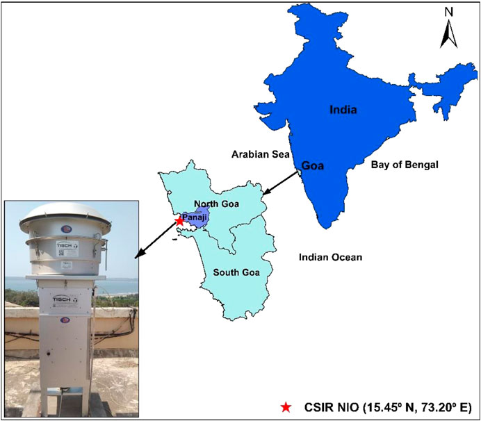
FIGURE 1. Location of bulk aerosol sampling at the roof of National Institute of Oceanography, Goa (at a height 56 m above sea level; 15.45°N, 73.20°E).

Methodology

Atmospheric aerosols with 50% cutoff aerodynamic diameter of 10 microns (PM₁₀) and 2.5 micron (PM_2.5) were collected on PALLFLEX™ Tissuquartz filters (8” × 10”) by using high-volume sampler (TISCH Environmental) at an average flow rate of 1.1 m³·min⁻¹. Few samples, between April 2018 and May 2018, were collected on Whatman-41 rectangular cellulose filters (20 × 25 cm) using same high-volume samplers. The sampler was set up on the terrace (15.45°N, 73.20°E) of NIO building at a height of 56 m from the ground level. Typically, each sample was collected by operating the sampler for 24-h with a sampling frequency of two samples per week. A total of 224 PM₁₀ and PM_2.5 samples (more details are in Table 1) were collected from December 2017 to February 2019. Prior to sample collection, quartz filters were conditioned in an oven at a temperature of 200°C for 3–4 h.

TABLE 1

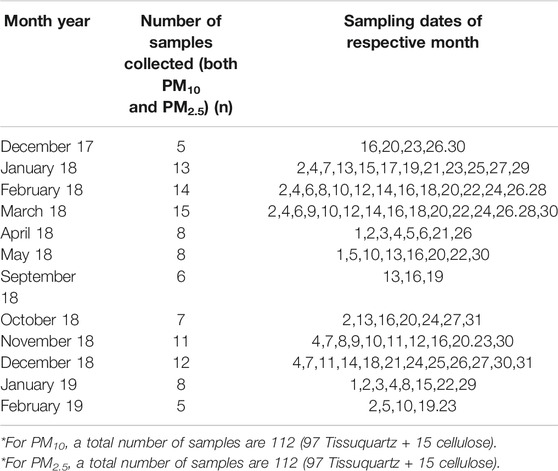
TABLE 1. Details of number of samples, sampling days in each month, and type of filter used for PM collection.

A piece (1/8th) of the filter sample was cut from the sampled area using a ceramic scissor under a clean laminar flow bench. This filter piece along with deionized water (Milli-Q; specific resistivity >18.2 MΩ-cm) was transferred into 50 ml Savillex bombs and subjected to ultrasonication for 30 min. The water extracts were subsequently filtered through a PVDF syringe filter with pore size 0.2 µm and then transferred to a preconditioned polypropylene bottle. This filtered solution was analyzed for cations (Na⁺, NH₄⁺, K⁺, Mg²⁺, and Ca²⁺) and anions (Cl⁻, NO₃⁻, and SO₄²⁻) using a thermo scientific ion chromatography system (Dionex ICS 5000). The cations (Na⁺, NH₄⁺, K⁺, Mg²⁺, and Ca²⁺) were analyzed using the analytical column IonPac CS12A, 4 × 250 mm, and guard column IonPac CG12A, 4 × 50 mm, using CSRS 300 as a suppressor. Methyl sulfonic acid has been used as an eluant for the cation analysis with a run time of 15 min. The anions (Cl⁻, NO₃⁻, and SO₄^2-) were analyzed using the analytical column IonPac AS16, 4 × 250 mm, and guard column IonPac AG16, 4 × 50 mm, using ASRS 300 as suppressor. 22 mM NaOH solution has been used as eluant for the anion analysis with the run time of 10 min. Merck multielement standard was used for standard preparation by suitably diluting it. Daily calibrations were done before starting the analyses, and fresh standards were prepared before analyses. Along with samples, field blanks were also extracted and analyzed using similar methodology as that of aerosol samples. The concentrations of ionic species were corrected for procedural blanks. Based on blank concentrations and average volume of air filtered (∼2000 m³), the detection limits for the water-soluble ionic species in aerosols were ascertained (18, 18, 20, 18, 25, 10, 30, and 30 ng·m⁻³ for Na⁺, NH₄⁺, K⁺, Mg²⁺, Ca²⁺,Cl⁻, NO₃⁻, and SO₄²⁻, respectively). The reproducibility in the analytical data for the measured concentrations is within 5% based on the repeat analysis of a number of samples and standards.

Meteorological data were obtained using an automatic weather system (AWS) installed at the roof top (∼56 m above the sea level) of the CSIR-National Institute of Oceanography (details of AWS are given in Mehra et al., 2005). In our study, we classified three different seasons 1) winter (WIN) during December–February; 2) summer (SUM) during March–May; and 3) post-monsoon (POM) during September–November, based on the previous studies (Agnihotri et al., 2015; Yadav et al., 2020) at this site. Using this classification, we computed 7-day air mass back trajectory (AMBT) ending at our study site for each sampling day (Figure 2). The AMBTs were computed using HYSPLIT-4 model and GDAS dataset of the National Oceanic and Atmospheric Administration Air Resource Laboratory (NOAA) at 500 m altitude (Stein et al., 2015). Supplementary Figures S1 and S2 depict the seasonal variation of temperature and relative humidity (RH), respectively. In winter, the average temperature was found to be 25°C with average RH of 72%, in summer average temperature was 28°C with average RH of 82%, and during post-monsoon average recorded temperature was 26°C with average RH of 90%. Although, we did not observe significant variation in temperature and relative humidity during different seasons, however, significant changes in wind trajectories were observed and discussed in detail in the next section.

FIGURE 2

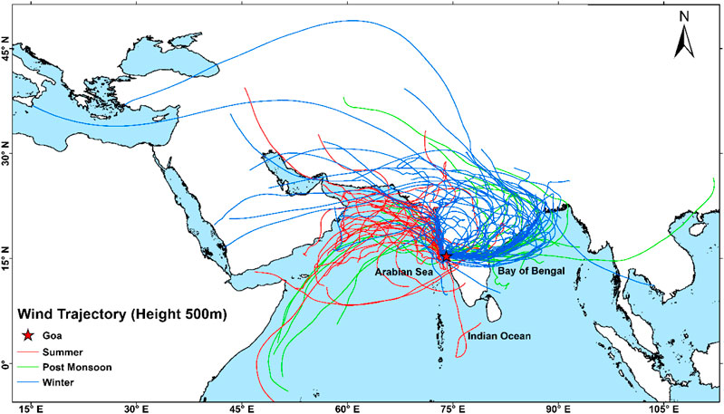
FIGURE 2. 7-day back trajectories at 500 m for sampling days ending at our sampling site. AMBTs were computed using the HYSPLIT-4 model and GDAS dataset of the National Oceanic and Atmospheric Administration Air Resource Laboratory (NOAA) at 500 m altitude (Stein et al., 2015) for this study.

Results and Discussion

Back-Trajectory Analyses

The AMBTs corresponding to different seasons, for sample collection days, are shown in Figure 2 with different colors. A distinct wind pattern is observed for WIN and SUM months; however, mixed winds are seen during POM season. Winds are mostly derived from marine region as well as Middle East deserts during SUM seasons, with several trajectories crossing over the coastal region of western India, Pakistan, and Iran–Pakistan border region. In contrast, winds during WIN season are mostly derived from continental locations in the Indian subcontinent, particularly from the Indo-Gangetic Plains (one of the hot spots for anthropogenic emissions during WIN; Thomas et al., 2019). Those derived during WIN are also observed to pass over the coastal region of eastern India as well as over the Bay of Bengal (Figure 2). After the southwest monsoon withdrawal, wind origin is observed from marine as well as continental locations, with few winds derived from coastal northwest Africa and far eastern part of the Bay of Bengal. In order to identify major contribution from emission sources during POM, we have done cluster analyses (Stein et al., 2015); all AMBTs computed during this period. Our analyses indicate the dominance of continental sources (more than 65%) as compared to marine sources (Supplementary Figure S3). It is interesting to note here that majority of winds at our study site indicate long-range transport trajectories possibly bringing aerosols derived from variety of sources including natural arid/semiarid desert and marine regions as well as polluted anthropogenic locations. Thus, it is apparent; meteorology may play an important role in impacting ambient aerosol composition leading to a strong seasonal variability at this location.

Seasonal Variability of Water-Soluble Ionic Composition in PM₁₀ and PM_2.5

In this study, a total of 224 aerosol samples were collected, which includes 112 PM₁₀ and 112 PM_2.5 samples (detail of number of samples, sampling days in each month, and type of filter used for PM collection is tabulated in Table 1). Water-soluble ionic composition (WSIC) is calculated by adding mass concentration (µg m⁻³) of all cations (Na⁺, NH₄⁺, K⁺, Mg²⁺, and Ca²⁺) and anions (Cl⁻, NO₃⁻, and SO₄^2-) measured in this study. The charge balance (in equivalent units) between total cations (∑⁺) and total anions (∑⁻) is used to assess reliability and quality of the WSIC data (Kumar et al., 2008a, Kumar et al., 2008b). A correlation plot between ∑⁺ and ∑⁻ is shown in Figure 3, wherein we observe most of the data are falling on or near to the 1:1 line for both PM₁₀ and PM_2.5 samples. We observe significant correlation between ∑⁺ and ∑⁻ for all PM₁₀ and PM_2.5 samples (r² is shown in Figure 3), except for some PM₁₀ and PM_2.5 (Figure 3) samples, particularly during SUM months. The equivalence ionic ratio (Σ⁻/Σ⁺) for PM₁₀ varied from 0.80 to 1.18 (mean: 1.00 ± 0.07) in WIN, 0.69 to 1.48 (mean: 0.99 ± 0.11) in SUM, and 0.91 to 1.26 (mean: 1.06 ± 0.07) in POM seasons. PM_2.5 samples show similar ratios ranging from 0.82 to 1.20 (mean: 0.98 ± 0.07), 0.64 to 1.16 (mean 0.97 ± 0.11), and 0.80 to 1.19 (mean: 1.01 ± 0.11) during WIN, SUM, and POM seasons, respectively. We observed some of the SUM samples (PM₁₀ and PM_2.5) are falling away from the 1:1 line toward the cation axis. Such deviation indicates anion deficit which can be attributed to the lack of measurement of bicarbonate ions which are mainly contributed by alkaline dust (Kumar et al., 2008a). The wind trajectories during SUM are mostly derived from the arid/semiarid desert region which can potentially bring mineral dust to our sampling site. Similar anion deficit has been reported by Kumar et al. (2008b) over the Bay of Bengal region during March–April 2006. In addition, several studies have suggested lack of measurement of organic anions which can contribute to the anion budget of ambient aerosols (Kulshrestha et al., 1998; Momin et al., 1999; Venkataraman et al., 2002; Rastogi and Sarin 2005).

FIGURE 3

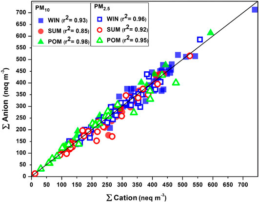
FIGURE 3. Seasonal correlation plot between total cation (sum of Na⁺, NH₄⁺, K⁺, Mg²⁺, and Ca²⁺) and total anion (sum of Cl⁻, NO₃⁻, and SO₄²⁻).

The seasonal variation of WSIC mass concentration for PM₁₀ and PM_2.5 is shown in Figure 4 using a box–whisker plot. WSIC concentration is found to be highest for WIN samples in PM₁₀ (mean: 25.5 ± 6.9; range: 10.4–50.0 μg m⁻³) followed by SUM (mean: 21.0 ± 4.6; range: 12.8–30.4 μg m⁻³) and POM (mean: 17.3 ± 9.1; range: 6.9–41.1 μg m⁻³) seasons. Similarly, WSIC in PM_2.5 is high for WIN (mean: 19.6 ± 5.8; range: 10.1–39.9 μg m⁻³); however, it is relatively higher during POM (mean: 14.4 ± 8.0; range: 2.3–29.0 μg m⁻³) than SUM (mean: 12.9 ± 7.3; range: 0.8–31.6 μg m⁻³) months. Compared to WIN and SUM, we observed large variability in WSIC during POM months, suggesting significant variability in sources, which is also supported by variation in AMBTs (Figure 2) during this period. Agnihotri et al. (2015) have reported on bulk aerosol chemical composition for WIN and SUM months during 2009–2011, wherein they observed high WSIC during SUM compared to WIN months. Another study by Yadav et al. (2020) have also observed higher WSIC for SUM than that in WIN for total suspended particulate (TSP or bulk) aerosol samples. However, they observed high WSIC in WIN compared to SUM for PM₁₀ and PM_2.5 samples during the year 2013 similar to our observation. The presence of sea salts, which are abundant in coarser fraction, contributes more during SUM (also supported by AMBTs) in the bulk samples as our sampling site is very near to coast. These coarser sea salts are relatively less collected on filters, while sampling using PM₁₀ and PM_2.5 inlets, as compared to bulk sampling. Thus, we (and previous studies) have observed higher WSIC for bulk during SUM than those collected with inlet of lower cutoff aerodynamic diameter.

FIGURE 4

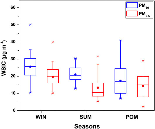
FIGURE 4. Seasonal variability of water-soluble ionic composition of PM₁₀ and PM_2.5 during the study period at Goa.

In order to assess the relative contribution of PM_2.5 WSIC to PM₁₀ WSIC, a scatterplot between PM₁₀ and PM_2.5 WSIC is shown in Figure 5 for all three seasons. It is evident that majority of SUM samples are falling away from the 1:1 line toward the PM₁₀ axis; however, POM and WIN samples are relatively near and/or on the 1:1 line. This suggests dominant contribution of fine mode WSIC toward water-soluble composition of PM₁₀ during WIN and POM months. However, during summer months, PM₁₀ mass could be dominated by coarser sea salt and mineral dust particles (more detail on their abundance in different size fractions is discussed in later section), which contribute relatively less to the PM_2.5 mass. This is also evident from the ratio of WSIC PM_2.5/WSIC PM₁₀, which is found to be relatively low (0.59 ± 0.24) during SUM compared to WIN (0.78 ± 0.14) and POM (0.76 ± 0.18) months. Our observation is consistent with those reported by Agnihotri et al. (2015), which highlighted predominance of the sea salt and mineral dust during SUM months compared to WIN season.

FIGURE 5

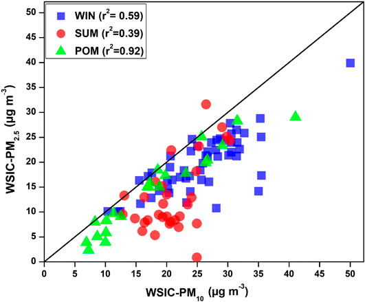
FIGURE 5. Scatter plot among PM_2.5 WSIC and PM₁₀ WSIC showing relative contribution of WSIC in PM_2.5 to PM₁₀ WSIC.

The percentage contribution of an individual water-soluble species to the total WSIC (of PM₁₀ and PM_2.5) is represented as pie charts (Figure 6) for the three different seasons. Sulfate (SO₄^2-) and ammonium (NH₄⁺) ions are dominant (contributing around 80% of WSIC for all season samples except for PM₁₀ SUM month) among anions and cations, respectively, in both fractions (Figure 6). A decrease in SO₄^2- contribution is observed for SUM samples (∼47%) in PM₁₀ compared to WIN and POM seasons; however, no significant variation is observed in SO₄^2- fraction for PM_2.5 samples (Figure 6). Similarly, no significant variation is observed for NH₄⁺ percentage in PM_2.5; however, a gradual increase in NH₄⁺ contribution to PM₁₀ is observed with lowest during SUM (10%), followed by POM (13%) and highest in WIN (16%). Apart from SO₄^2- and NH₄⁺, we observe significant contribution of Ca²⁺, Na⁺, Cl⁻, and NO₃⁻ to PM₁₀, particularly during SUM months, and K⁺ in PM_2.5 samples. These observations suggest contribution of primary emission (mainly from sea salt and mineral dust) is significant in PM₁₀, while those from secondary aerosol formation (formed by gas to particle conversion or multiphase chemistry) may be dominant in PM_2.5, which is consistent with previous studies from the Indian subcontinent (Kumar and Sarin, 2010b; Ram et al., 2012; Rastogi et al., 2015).

FIGURE 6

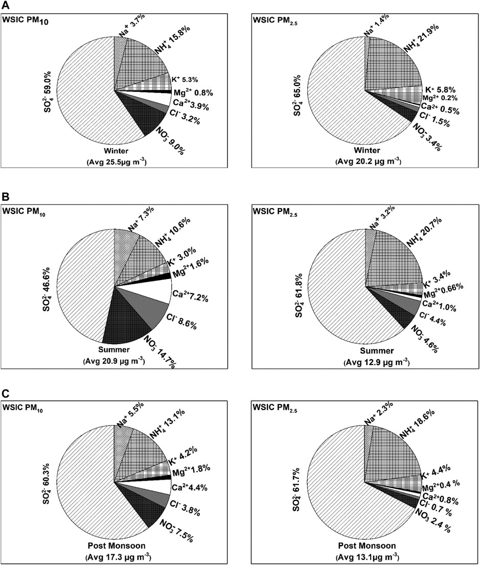
FIGURE 6. Pie chart showing relative contribution of individual ionic species to the total WSIC in PM₁₀ and PM_2.5 during (A) winter, (B) summer, and (C) post-monsoon (see text for season description).

Chemical Species of WSIC and Their Variation in PM₁₀ and PM_2.5

Sea Salt (Na⁺ and Cl⁻)

Sea salts are mainly derived from breaking of sea waves in the marine region (Anguelova and Webster, 2006). By using Na⁺ and Cl⁻ concentration in ambient aerosols, sea-salt concentration can be estimated, presuming that Na⁺ and Cl⁻ ions solely derived from seawater, following this relation (Quinn et al., 2007; Kumar et al., 2008a):

$\text{Sea Salt}=\left[{\text{Cl}}^{-}\right]\left(\text{μg}{\text{m}}^{-3}\right)+1.47\ast \left[{\text{Na}}^{+}\right]\left(\text{μg}{\text{m}}^{-3}\right).$

Here, 1.47 is the ratio of (Na⁺+ K⁺+Mg²⁺+ Ca²⁺+SO₄^2- + HCO₃⁻)/Na⁺ in seawater (Holland, 1978; Quinn et al., 2004). This approach excludes the contribution of nss-K⁺, Mg²⁺, Ca²⁺, SO₄², and HCO₃⁻ in the sea-salt mass and allows for the loss of Cl⁻ due to its depletion through chemical reaction. The monthly average trend of sea-salt concentration is shown in Figure 7, as the box–whisker plot and their season average concentration are reported in Tables 2 and 3. A large variation is observed for PM₁₀ samples with higher concentration during SUM season (3.73 ± 1.7 μg·m⁻³) than WIN (1.89 ± 0.87 μg·m⁻³) and POM (1.70 ± 1.29 μg·m⁻³) period. On the other hand, no significant variation is found for PM_2.5 samples except few higher episodic values at the beginning of summer months (March 2018 and February 2019). These episodic higher values may be attributed to stronger winds from marine region bringing coarse and fine sea salts to our sampling site, which is also evident from higher sea-salt concentrations in PM₁₀ for March 2018 and February 2019 (Figure 7). An increase in sea-salt concentration depends on higher wind speed as well as wind direction and oceanic waves (de Leeuw et al., 2000; Niedermeier et al., 2014). During this study, we have observed relatively higher wind speed during summer months than rest of the year. In addition, the winds are mainly derived from marine region during summer, as evident from the AMBTs (Figure 2). Thus, the higher values of sea salt can be attributed to the meteorological condition prevailing at our study site. It is important to mention here that sea salts also contribute to other ions (eg, K⁺, Mg⁺², Ca²⁺, and SO₄^2-), and thus, sea-salt correction is necessary to assess their temporal variability. The non–sea-salt (nss) components have been calculated by using the following equations:

$\text{nss}\mathrm{-}\text{X}={\left[\text{X}\right]}_{\text{total}}\mathrm{-}{\text{Rx}}_{\text{sea}\mathrm{-}\text{salt}}\text{*}{\left[{\text{Na}}^{+}\right]}_{\text{measured}},$

where [X]_total is measured concentration of specific ion, Rx_sea-salt is the weight ratio of particular ion to Na⁺ in seawater, and [Na⁺] _measured is measured Na⁺ concentration in ug m⁻³. Rx_sea-salt for K⁺, Ca²⁺, Mg²⁺, and SO₄^2- is 0.037, 0.0373, 0.12, and 0.252, respectively (Keene et al., 1986; Kumar and Sarin, 2009; Sarin et al., 2011).

FIGURE 7

FIGURE 7. Box–whisker plots representing the monthly mean (solid line) and different percentile levels (95th, 75th, 25th, and 5th) of sea-salt concentrations during the study period. Different seasons are on the top x-axis.

nss-Ca²⁺ and nss-Mg²⁺

The presence of nss-Ca²⁺ and nss-Mg²⁺ ions in the ambient aerosol samples typically indicates the contribution of crustal mineral dust (Rastogi and Sarin, 2006; Kumar and Sarin, 2010b). Monthly average concentration and its variation for nss-Ca²⁺ and nss-Mg²⁺ are shown in the box–whisker plot (Figure 8), and their seasonal average for PM₁₀ and PM_2.5 is reported in Tables 2 and 3. A general increasing trend can be observed in PM₁₀ particles for nss-Ca²⁺ concentration (in μg·m⁻³) while moving from WIN (mean: 0.93 ± 0.64; range: 0.36 – 3.7) to SUM (mean: 1.31 ± 0.72; range: 0.36 – 2.88) season, and then, it again starts decreasing in POM (mean: 0.67 ± 0.4; range: 0.11 – 0.14) with an average comparable value with winter month of 2019. No such significant temporal variability is observed for PM_2.5. However, relatively lower values (mostly below detection (BD) were found for nss-Mg²⁺ (Table 3), with no significant temporal variability as observed for that of nss-Ca²⁺. Higher concentration of sea-salt corrected calcium during SUM can be attributed to contribution from the arid/semiarid desert region in the Middle East (Arabian Peninsula, region bordering Afghanistan–Iran–Pakistan, Sistan Basin) as well as desert region in northwestern India (Thar Desert). Air mass back trajectories are clearly observed to transverse over these regions (Figure 2) during the SUM months. In contrast, we observe mixed air masses with dominant contribution from the continent (based on cluster analyses; Supplementary Figure S3) during POM, as well as air mass from northern/northeastern India during WIN, can transport mineral dust contributing to nss-Ca²⁺. In contrast to other locations over India (Kumar and Sarin, 2010b; Ram et al., 2010), we did not observe significant variation in nss-Ca²⁺ during the annual seasonal cycle. For example, over Mt. Abu, a high-altitude site located in western India, increase in summer nss-Ca²⁺ is observed by a factor of two or more than those observed in monsoon and winter seasons (Kumar and Sarin, 2010b). Similarly, Ram et al. (2010) have observed an order of magnitude increase in nss-Ca²⁺, over Kanpur. However, there are occurrence of dust storms in the Middle East and southwest Asia region (Aswini et al., 2020b; Kumar et al., 2020) which can also significantly contribute to nss-Ca²⁺ over our study site. Similar kind of trend for Ca²⁺ was also reported in Agnihotri et al. (2015) (winter: 2.3 ± 1.4) and in Yadav et al. (2020) (WM: 1.45 ± 0.57; SIM: 2.79 ± 2.22).

FIGURE 8

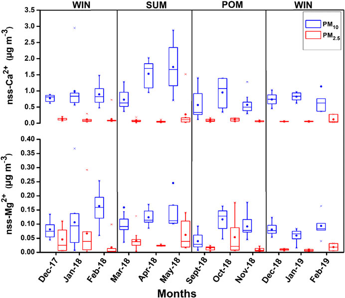
FIGURE 8. Box–whisker plots showing monthly variation of nss-Ca²⁺ and nss-Mg²⁺ during the study period.

TABLE 2

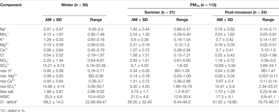
TABLE 2. Seasonal average concentration (in μg m⁻³) of water-soluble PM₁₀ components during the present study.

TABLE 3

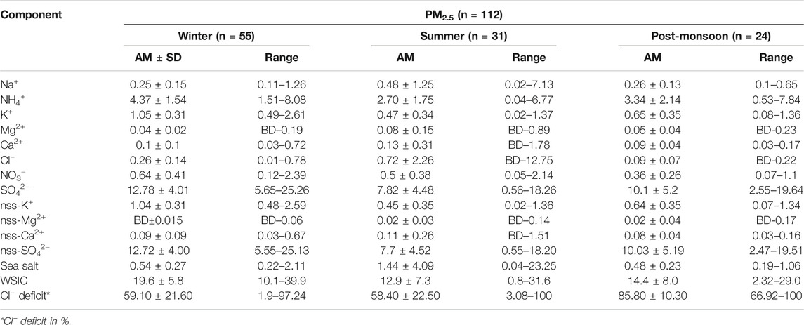
TABLE 3. Seasonal average concentration (in μg m⁻³) of water-soluble PM_2.5 components during the present study.

Secondary Inorganic Species (NH₄⁺, NO₃⁻, and nss-SO₄²⁻)

Secondary inorganic species are mainly formed via multiphase chemistry from the precursor gases (ammonia and oxides of sulfur and nitrogen) which are emitted mostly from anthropogenic (fossil fuel and biomass burning) emissions (Seinfeld and Pandis, 2006; Zheng et al., 2020). These secondary species play a vital role in influencing several atmospheric processes acid uptake, enhancing aerosol Fe solubility (Rastogi and Sarin, 2006; Kumar and Sarin, 2010b) impacting on the overall climate in short-term and long-term timescales (Zheng et al., 2020). The monthly distribution of all secondary species is shown as box–whisker plots in Figure 9 and their seasonal average concentration with minimum and maximum values in PM₁₀ and PM_2.5 are detailed in Tables 2 and 3, respectively. The NH₄⁺ and nss-SO₄²⁻ ions were found to covary throughout the year with almost similar concentration in PM₁₀ and PM_2.5. This indicates a significant and dominant contribution of inorganic ions in PM_2.5, which is also evident from the plot shown in Supplementary Figures S4 and S5, respectively. Majority of data are falling on or near to 1:1 line, toward PM_2.5, which indicate their dominance in PM_2.5. Furthermore, we observed higher values during WIN (PM₁₀ NH₄⁺ mean: 4.15 ± 1.67; range: 0.95–7.48, PM_2.5 NH₄⁺ mean: 4.37 ± 1.54; range: 1.51–8.08, PM₁₀ nss-SO₄^2- mean: 14.98 ± 4.74; range: 5.06–30.7, and PM_2.5 nss-SO₄²⁻ mean: 12.72 ± 4.00; range: 5.55–25.13) which gradually decreases in SUM (PM₁₀ NH₄⁺ mean: 2.24 ± 1.33; range: 0.29 – 5.40, PM_2.5 NH₄⁺ mean: 2.70 ± 1.75; range: 0.04 – 6.77, PM₁₀ nss-SO₄^2- mean: 9.30 ± 4.50; range: 1.66 – 19.79, and PM_2.5 nss-SO₄²⁻ mean: 7.77 ± 4.52; range: 0.55 – 18.20) to lowest value (in May 2018) and start to increase from October 2018 onward in POM to higher values in WIN 2019. Thus, a clear seasonality can be witnessed from this; however, long-term observation can provide a more robust picture on seasonal variability of these species. Higher concentration of sulfate and nitrate during WIN months can be attributed to local anthropogenic activities as well as winds from the northeastern region of India and/or Indo-Gangetic Plains (IGP), which are relatively more polluted regions, particularly during winter months (Ram et al., 2010). The AMBTs are observed to be derived from the emission regions located in the IGP. However, relatively lower concentration in summer is due to dilution of local anthropogenic emission by relatively pristine air parcel emanating from the marine region (Figure 2), leading to lower concentrations. In post-monsoon season, initially, the concentration is less but gradually increases in October and November months. This is due to winds which are coming from the southwest during monsoon period were getting reversed to northeast winds as evident from the air mass back trajectories shown in Figure 2. This high contribution of nss-SO₄²⁻ during winters suggest a significant component of secondary inorganic aerosols resulting from emissions of SO₂ by a variety of combustion sources using sulfurous fuels, such as coal and oil which is long range transported by winds from the continental region. However, in summer, although the concentration is very low, still most of the winds are coming from the marine region which depicts that nss-SO₄²⁻ may be derived from oxidation of DMS (dimethyl sulfide).

FIGURE 9

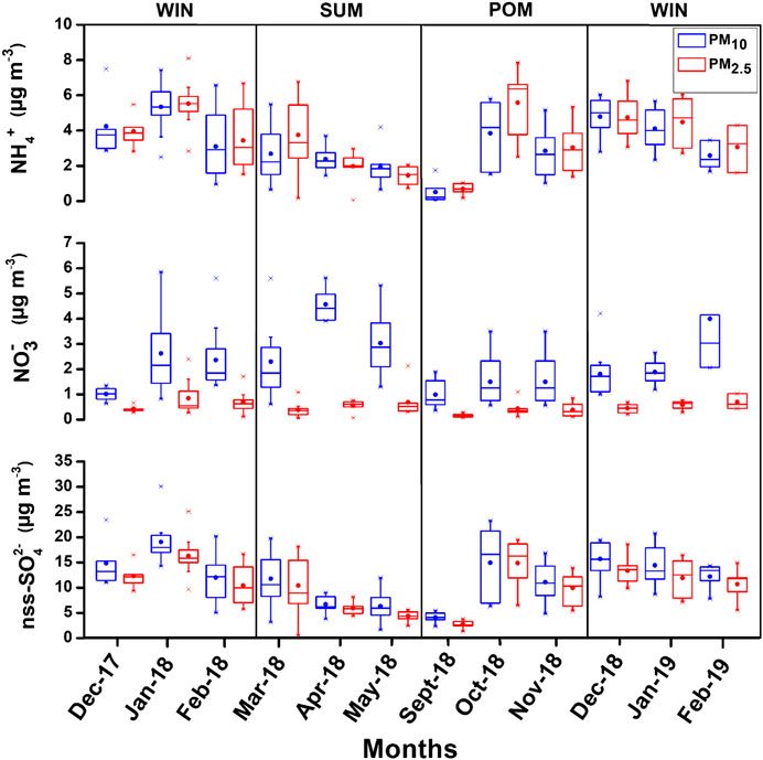
FIGURE 9. Box–whisker plots showing monthly variation of secondary ionic species (NH₄⁺, NO₃⁻, and nss-SO₄²⁻) ions in the present study.

In contrast to sulfate and ammonium ions, NO₃⁻ is found almost negligible in PM_2.5 as compared to PM₁₀ (Figure 9; Tables 2 and 3; Supplementary Figure S6). Moreover, no significant seasonal variability is found for NO₃⁻ and similar seasonal average observed for WIN (mean: 2.25 ± 1.44; range: 0.64 – 8.67) and SUM (mean: 2.93 ± 1.51; range: 0.61 – 5.60) which are relatively higher than POM (mean: 1.16 ± 0.72; range: 0.36 – 3.5) for PM₁₀ samples. NO₃⁻ is generally formed by the oxidation of NO_x (Wang et al., 2006). This formation of NO₃⁻ involves the gas-to-particle conversion of NO_x in the ambient atmosphere. Ooki and Uemastu (2005) reported that nitrate is the dominant constituents associated with the mineral dust rather than the nss-SO₄^2-. Relatively higher abundance of nitrate is observed for PM₁₀ than PM_2.5 (shown in the box–whisker plot; Figure 9) during this study and may be attributed to their association with coarser dust as well as sea-salt particle. However, it is not possible to decouple the relative contribution of sea salt and dust in neutralizing nitrates in the coarse mode using our chemical composition data. Yadav et al. (2020) have reported higher abundance of nitrate in PM₁₀ and bulk samples, as compared to PM_2.5, at coastal site on eastern (Vizag) and western (Goa) North Indian Ocean. Similar enhanced abundance has been found by several studies at high-altitude pristine sites (Kumar and Sarin, 2010b) and polluted the Indo-Gangetic Plains (Ram et al., 2010).

Biomass Burning Species (nss-K⁺)

Studies have indicated that concentration of sea-salt corrected potassium (nss-K⁺) in fine mode aerosols can serve as a diagnostic tracer for biomass burning source (Andreae, 1983; Andreae and Marlet, 2001). However, its contribution from sea salts and dust sources is highly variable for regional case studies with its dominance in the coarse fraction. Galanter et al. (2000) estimated the geographical distribution of biomass burning to be fairly uniformly distributed over the Indian subcontinent with a maximum in the northeastern parts. They also estimated that the biomass burning in India takes place mainly during winter and summer (January–May). The monthly average trend for nss-K⁺, in both size fractions, is shown in Supplementary Material S3. In this study, it was found that nss-K⁺ ion contribution was found to be maximum during WIN (Supplementary Figure S7), that is, ranged from 0.16 to 2.71 μg·m⁻³ (Mean: 0.95 ± 0.38 μg·m⁻³) and minimum during SUM ranged from BD to 1.28 μg·m⁻³ (Mean: 0.34 ± 0.26 µg·m⁻³) (Supplementary Figure S7). During post-monsoon season, nss-K⁺ ion ranged from BD to 1.47 (Mean: 0.54 ± 0.38 µgm⁻³) in PM₁₀ particles. Similarly, in PM_2.5 its abundance is maximum in winters, that is, ranged from 0.48 to 2.59 μg·m⁻³ (Mean: 1.04 ± 0.31 μg·m⁻³) and minimum in summer 0.02 to 1.36 μg·m⁻³ (Mean: 0.45 ± 0.35 μg·m⁻³). It is important to highlight here that the relative contribution of nss-K⁺ of fine fraction is more than 90% to total PM₁₀ nss-K⁺. This is evident from the PM_2.5-nss-K⁺/PM₁₀-nss-K⁺ ratio, which is found to be 0.94 ± 0.12, 0.96 ± 0.17 and 0.99 ± 0.03, during WIN, SUM, and POM seasons. This observation further suggests the dominance of biomass burning tracer in fine fraction as compared to coarser one, particularly during WIN and POM seasons, when relatively higher concentrations are found as compared to SUM period. This further points to contribution from long-range transport of aerosols derived from polluted IGP region impacting at the coastal region of the Arabian Sea and corroborated by back trajectories during WIN and POM seasons.

Major Sources of Aerosols Over Goa

We have observed seasonal variability of various chemical species, and their variations have been largely attributed to the distinct wind patterns, primarily discerned by the air mass back trajectories, during the whole year. In this section, we will further attempt to assess the sources of different chemical species and its relations with meteorology (mainly AMBTs). The NO₃⁻/nss-SO₄²⁻ ratio typically gives an idea about the contribution from the mobile sources (vehicular emissions) vis-à-vis stationary sources (industrial emissions) (Arimoto et al., 1996; Kumar and Sarin, 2010b; Yadav et al., 2020). In this study, the consistently lower ratio (<1) reveals that major contribution of anthropogenic activities is from stationary sources during all the seasons for both the particle classes PM₁₀ and PM_2.5. It is noteworthy that during WIN in PM_2.5, the mean ratio is 0.05 ± 0.04 which is almost 3 times lower than the ratio in PM₁₀ 0.17 ± 0.0.16. This is due to increase in concentration of nss-SO₄²⁻ in the fine mode aerosol by long-range transport from the Indo-Gangetic Plains (IGP) region which is also supported by our back-trajectory analysis. On the contrary during SUM, the mean ratio was 0.61 ± 0.29 for PM₁₀ which is almost 7 times higher than that for PM_2.5 (0.09 ± 0.10). This is due to increase in NO₃⁻ concentration in PM₁₀ and its uptake by coarser mineral dust and sea-salt particles. An enhanced transport of sea salt and mineral dust is evident from the increase observed in Na⁺ and nss-Ca²⁺ concentration during summer season, which is further supported by the AMBTs (Figure 2) deriving from desert and marine regions. These observations are found to similar to those reported by Kumar and Sarin (2010b) highlighting the role of long-range transport of nss-SO₄²⁻ associated with NH₄⁺ in fine mode and NO₃⁻ (associated with crustal species sea salts). The scatterplot between mass concentrations of nss-SO₄²⁻ and NH₄⁺ (Supplementary Figure S8) shows a significant correlation for all season, particularly in PM_2.5. This clearly suggests the favorable association between secondary sulfate and ammonium ions. We also observed a better correlation between NO₃⁻ and nss-Ca²⁺ + nss-Mg²⁺ + Na⁺ (Supplementary Figure S9), which establishes association of nitrates with dust and sea salt, particularly in coarser fraction.

The AMBTs during SUM and POM were mostly derived from the desert region, which are sources of mineral dust; a concomitant increase in nss-Ca²⁺ concentration has been observed during SUM and POM, particularly in PM₁₀ fraction. However, no such variability is found for nss-Mg²⁺. Moreover, very low concentration of nss-Mg²⁺ is found for PM_2.5 throughout the year (Table 2). A scatterplot between nss-Ca²⁺ and nss-Mg²⁺ in PM₁₀ (Supplementary Figure S10) exhibits relatively poor correlation, highlighting different sources of Ca²⁺ and Mg²⁺ ions. Similar observations were reported by Yadav et al. (2020) for aerosols collected at Goa and suggested distinct sources of these ion, which is in contrast to those observed at a semiarid location in western India (Kumar and Sarin, 2010b). Such poor correlation can be also attributed to relative contribution of different minerals (calcite vs dolomite) and their chemical processing during long-range transport (Rastogi and Sarin, 2006). Apart for the ions discussed above, the nss-K⁺ (typically considered as tracer for biomass burning emissions) concentration is found to be high during end of POM and WIN months (Supplementary Figure S7). We noticed a sharp increase in its concentration from September to October and further increase in November. This increase in nss-K⁺ is also associated with change in wind trajectories from southwesterly to northeasterly as southwest monsoon recedes and northeast monsoon picks up. During October–November months, crop residue burning is very frequent in the northwestern regions (Punjab, Haryana, and western Uttar Pradesh) of India. The emissions from these sources spread in all directions through long-range transport mechanisms, depending upon the meteorological conditions (Sarkar et al., 2018). Due to change in wind regime, we observe a significant increase in nss-K⁺. This observation further attests to the fact that meteorology plays an important role in impacting aerosol concentration and composition at our sampling site.

Interaction Between Primary and Secondary Aerosols in PM₁₀ and PM_2.5

Chloride Deficit

Sea salt undergoes heterogeneous phase reaction while interacting with acidic gases and/or secondary aerosols (eg, HNO₃ and H₂SO₄) causing removal of nascent chlorine via supersaturation of HCl, and this is referred as Cl⁻depletion (Sarin et al., 2011). This is significant over the marine or coastal regions due to the impact of polluted air mass interacting with sea salts (Struges and Shaw, 1993; Johansen et al., 1999; Kumar et al., 2008a, Kumar et al., 2008b). Such depletion and emission of reactive chloride (as a free radical) is considered to be an important intermediate in the oxidation reactions associated with the removal of light hydrocarbons and ozone in the atmosphere (Singh and Kasting 1988; Vogt et al., 1996). Cl⁻ depletion (%) can be calculated by the following relation (Sarin et al., 2011):

${\text{Cl}}^{\mathrm{-}}\text{depletion }\left(\text{\%}\right)=100\left[\left(1\text{.}80\times {\text{Na}}^{+}\right)\mathrm{-}{\text{Cl}}_{\text{m}}^{\mathrm{-}}\right]/\left(1\text{.}80\times {\text{Na}}^{+}\right),$

where 1.80xNa⁺ is the Cl⁻ concentration (µg m⁻³) expected from the sea and Cl⁻_m is the measured Cl⁻ concentration (µg m⁻³) in the sample. In the present study, we observed lower Cl⁻/Na⁺ ratio than bulk seawater ratio of 1.80 indicating the Cl⁻−depletion process, which is observed in all seasons for both PM₁₀ and PM_2.5. This is also evident from the scatterplot between mass concentrations (in μg m⁻³) of Na⁺ and Cl⁻, shown in Figure 10 for all seasons. We observe large scatter in the dataset, showing significant variability in the Cl⁻ depletion process at our study site. Majority of PM₁₀ data are falling near to the seawater line, particularly during the SUM season; however, large deviation (from seawater line) is observed for WIN and POM samples. Similar distribution is found for PM_2.5 data, although the sea-salt concentration is relatively lower than those observed for PM₁₀ (see Section Sea Salt salt (Na⁺and Cl⁻)). The Cl⁻/Na⁺ ratio for PM₁₀ was found to be lowest (mean: 0.60 ± 0.30) during WIN as compared to those in POM (mean: 0.75 ± 0.44) and SUM (Mean: 0.82 ± 0.64). However, in PM_2.5, we observe lowest ratio in POM (0.41 ± 0.28) compared to almost similar ratio in WIN (1.02 ± 0.48) and SUM (1.09 ± 0.56). This indicates relatively high Cl⁻-depletion in PM₁₀ (mean = 68.2 ± 14.3%) compared to PM_2.5 (mean = 59.1 ± 21.6%) during WIN, almost similar in both fractions (PM₁₀ mean = 56.2 ± 32.4% and PM_2.5 mean = 58.4 ± 22.5%) during SUM, and high in PM_2.5 (mean = 85.8 ± 10.3%) compared to PM₁₀ (mean = 61.5 ± 18.8%) during POM. This is also evident in Figure 11, showing average monthly trend of Cl⁻ depletion. Similar variations (39–78%) in Cl⁻ deficit have been reported by Venkataraman et al. (2002) at an urban site (Mumbai, 19°23′N and 72°50′E) on west coast of India in two different sampling periods during January–March. In contrast to such variable Cl deficit, Sarin et al. (2011) have observed very high deficit (ranging from 82 to 98%) during continental outflow season over the Bay of Bengal. However, large variability (12–100%) has been reported by Kumar et al. (2008a) over the Arabian Sea. Such observation clearly demonstrates the role of continental outflow in removing Cl⁻ from sea salt which has significant implication toward atmospheric chemistry in the marine atmospheric boundary layer. The released chlorine have potential as an oxidant (Solomon, 1999), which may have role in oxidation of dimethyl sulfide (DMS; Keene et al., 1986) as well as in enhancing tropospheric ozone due to their interaction with volatile organic compounds (Raff et al., 2009). In comparison to such high deficit, several studies (Savoie and Prospero 1982; Kerminen et al., 1998; Johansen et al., 1999) have observed relatively lower values (ranging from 20 to 30%) in open oceanic regions and have attributed to chemical uptake of nss-SO₄²⁻ derived from DMS sources in the open ocean. In this study, we have not measured the methane sulfonate ions; thus, we could not estimate the DMS derived (or biogenic sourced) sulfate.

FIGURE 10

FIGURE 10. Scatterplot between Na⁺ and Cl⁻ mass concentration in three seasons at coastal sampling station, Goa. The data point falling away from the seawater line indicates the Cl⁻ depletion process.

FIGURE 11

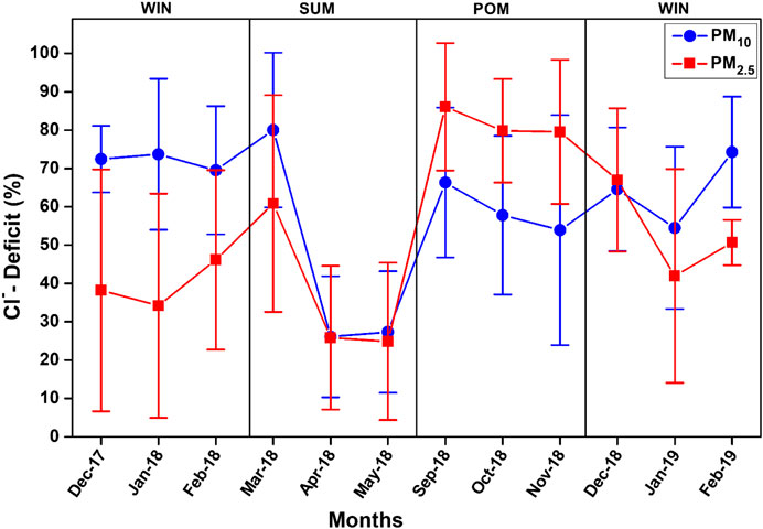
FIGURE 11. Variation of monthly average chloride deficit (%) in PM₁₀ and PM_2.5 during the study period.

As discussed previously, acidic species (nitrate and sulfate) play vital role in controlling this process; we will assess their contribution in different size fractions. A scatterplot between equivalent concentrations of (Cl⁻ + NO₃⁻) and Na⁺ is shown in Figure 12A, to understand the role of nitrate in Cl⁻ removal following Sarin et al. (2011). In contrast to the observation of Sarin et al. (2011) over the Bay of Bengal, we observed scatter of data on either side of 1:1 line, suggesting the role of both sulfate and nitrate in the Cl⁻ removal process. The concentration of sulfates is 3–10 times higher than nitrates in PM₁₀ and order of magnitude is higher in PM_2.5, which suggests sulfate ions are mostly responsible for the Cl⁻ removal process. However, we noticed majority of PM₁₀ samples during all season to fall toward the (Cl⁻+NO₃⁻), suggesting contribution from nitrates in controlling this process. The role of nitrate in removing sea-salt chloride is well documented in various studies (Wu and Okada, 1994; Quinn and Bates, 2005; Hsu et al., 2007), particularly in coarser fraction compared to fine mode (Pio and Lopes, 1998). In this study, we observed relatively higher ratios of [Cl⁻+NO₃⁻] to Na⁺ for WIN (mean: 0.91 ± 0.21) and POM (mean: 0.79 ± 0.24) in PM₁₀ than their PM_2.5 counterpart (0.79 ± 0.21 and 0.59 ± 0.20, respectively). However, during SUM, relatively higher ratio is observed for PM_2.5 (mean: 0.94 ± 0.31) than PM₁₀ (mean: 0.74 ± 0.30). These observations suggest contribution from nitrate in removing Cl⁻ from sea salt, as the overall ratios are higher than those observed for the Bay of Bengal (0.37) (Sarin et al., 2011) and the subtropical South China Sea (0.17) (Hsu et al., 2007), where the role of nss-SO₄²⁻ is dominant in controlling this process. We further examined the relationship between NH₄⁺ and nss-SO₄²⁻ (in equivalent units; Fig. 12b), where we observed most of the PM₁₀ and PM_2.5 data are falling on or nearby 1:1 line, indicating a complete neutralization by ammonium ions. The NH₄⁺/nss-SO₄²⁻ ratio was found to be greater than one in PM_2.5 during WIN and SUM (1.47 ± 0.14 and 1.06 ± 0.60, respectively) as well as in PM₁₀ (1.32 ± 0.23 and 1.09 ± 0.29, respectively). This indicates formation of (NH₄)₂SO₄ as compared to (NH₄)HSO₄ in PM₁₀ as well as in PM_2.5 during WIN and SUM seasons. In contrast, relatively lower ratios were observed for POM (0.81 ± 0.47 for PM₁₀ and 0.92 ± 0.31 for PM_2.5), which suggest the abundance of (NH₄)HSO₄ instead of (NH₄)₂SO₄ or relatively more acidic nature of aerosols controlled by sulfates. We have also observed higher Cl⁻deficit during POM than SUM and WIN, which can thus be attributed to this excess sulfates over and above that is neutralized by NH₄⁺. Based on cluster analyses (Supplementary Figure S3), we have observed AMBTs are mostly derived from the continental sources during POM, and the presence of excess nss-SO₄²⁻ can impact other processes which include chemical processing of iron present in ambient aerosols. This has significant implication to the supply of labile Fe, which can act as micronutrients, to coastal waters of the Arabian Sea.

FIGURE 12

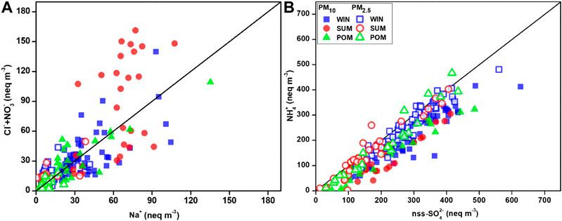
FIGURE 12. Scatterplot between (A) Cl⁻ + NO₃⁻ vs. Na⁺; (B) NH₄⁺ vs nss-SO₄²⁻ (in equivalence unit), highlighting the role of secondary species in removal of chloride from sea-salt particle.

Neutralization Factor

Neutralization factor (NF) is an indicator of aerosol acidity, and it can be estimated from the ratio of molar concentrations of cations and anions (Wu et al., 2017; Yadav et al., 2020). In this study, considering the significant contribution of nss-Ca²⁺, nss-Mg²⁺, and nss-K⁺, we have used equation for calculation of the NF following Yadav et al. (2020), which is

$\text{NF }=\left(\left[{\text{NH}}_4^{\mathrm{+}}\right]+\left[{\text{Na}}^{+}\right]+2\text{*}\left[{\text{nss}-\text{Ca}}^{2+}\right]+2\text{*}\left[{\text{nss}-\text{Mg}}^{2+}\right]+\left[\text{nss}-\text{K}+\right]\right)/\left(2\text{*}\left[{\text{nss}-\text{SO}}_4^{2\mathrm{-}}\right]+\left[{\text{NO}}_3^{\mathrm{-}}\right]+\left[{\text{Cl}}^{\mathrm{-}}\right]\right).$

Here, all the ionic concentrations are in µeq m⁻³. A value of NF < 1 indicates acidic nature of an ambient aerosol and/or incomplete neutralization; however, a value of NF > 1 indicates that cations are involved in neutralizing the acidic species of aerosol (Wu et al., 2017). We observed the NF averaging around 1 for PM_2.5 (1.00 ± 0.20) except for those collected during POM (0.97 ± 0.11), suggesting a complete neutralization of acidic species in ambient aerosols during WIN and SUM months. Being NH₄⁺, the dominant cation, it plays a key role in neutralizing the acidic species during WIN and SUM in PM_2.5. However, either due to lack of ammonium or excess nss-SO₄²⁻, we observe an incomplete neutralization during the POM season. Similarly, near neutrality of ionic species is found for PM₁₀ during WIN (0.96 ± 0.07) and SUM (0.97 ± 0.12) months. However, relatively lower NF (0.90 ± 0.07) is shown by POM samples, highlighting the presence of excess acid (more than neutralized by alkaline species). This excess acid can significantly impact other atmospheric processes including Cl⁻-depletion. It is interesting to note here that we have observed relatively higher Cl⁻ deficit in PM₁₀ and PM_2.5 during the POM season, which is corroborating our previous interpretation of high Cl deficit (see Section Chloride Deficit). We further compared our results with Yadav et al. (2020), wherein they have reported near neutrality for both PM₁₀ and PM_2.5 and lower NF for TSP suggesting acidic composition at Goa. These results further highlights on increase in neutralization process with decrease in particle grain size (Wu et al., 2017), which is consistent with our observation as well.

Conclusion

We present here a one-year long aerosol chemical composition data of size-segregated aerosols (PM₁₀ and PM_2.5) at a costal location in the northeastern Arabian Sea (Goa; 15.45°N, 73.20°E, 56 m above the sea level). Following are the major outcomes of our study:

1. A uniform dominance of nss- SO₄²⁻ and NH₄⁺ is observed in both PM₁₀ and PM_2.5 in all three seasons, with highest abundance of both species during winter months.

2. A significant temporal variability is observed in sea-salt concentration in PM₁₀ with highest values observed during summer, while no significant temporal variability is found for PM_2.5 composition.

3. Significant increase in secondary aerosols (SO₄²⁻ and NH₄⁺) is observed in PM_2.5, during winter associated with higher values of nss-K⁺ indicating long-range transport of secondary aerosols from the north/northwestern India (IGP). This observation is corroborated with air mass back-trajectory analyses.

4. A remarkable contribution by excess of acidic ions is observed being responsible for significant chloride depletion which is highest during post-monsoon months for fine mode aerosols.

5. Neutralization factor is found to be lowest during post-monsoon; however, near neutrality is observed for rest of the year.

In addition to confirming the results of previous studies based on shorter measurement periods, this study has regional as well as global importance as it provides quality dataset on aerosols water-soluble ionic composition at a regional location in the northeastern Arabian Sea. Such dataset is helpful in constraining output of the climatic models and gives more realistic future projections.

Data Availability Statement

The original contributions presented in the study are included in the article/Supplementary Material, further inquiries can be directed to the corresponding author.

Author Contributions

AnK: methodology, investigation, and writing-original draft. AsK: conceptualization, investigation, writing-original draft, resources, project administration, and funding acquisition. MA: methodology and data analyses. PP: methodology and data analyses. GS: methodology and data analyses. NG: Review and Editing.

Funding

Funding for this research is supported by MoES PMN project. The Department of Science and Technology funded AsK, Govt. of India, under the SPLICE Program (Grant No. DST/CCP/Aerosol/85/2017(G)).

Conflict of Interest

The authors declare that the research was conducted in the absence of any commercial or financial relationships that could be construed as a potential conflict of interest.

Acknowledgments

We gratefully acknowledge the NOAA Air Resources Laboratory (ARL) for the provision of the HYSPLIT transport and dispersion model (http://www.ready/noaa.gov) used in this publication. We thank K. Suresh and Udisha Singh for the support during analyses of water soluble ionic species. NIO contribution no. is 6662.

Supplementary Material

The Supplementary Material for this article can be found online at: https://www.frontiersin.org/articles/10.3389/fenvs.2020.619174/full#supplementary-material.

References

Agnihotri, R., Karapurkar, S. G., Sarma, V. V. S. S., Yadav, K., Kumar, M. D., Sharma, C., et al. (2015). Stable isotopic and chemical characteristics of bulk aerosols during winter and summer season at a station in Western Coast of India (Goa). Aerosol Air Qual. Res. 15, 888–900. doi:10.4209/aaqr.2014.07.0127

CrossRef Full Text | Google Scholar

Anderson, R. F. (2020). GEOTRACES: accelerating research on the marine biogeochemical cycles of trace elements and their isotopes. Ann. Rev. Mar. Sci. 12, 49–85. doi:10.1146/annurev-marine-010318-095123

PubMed Abstract | CrossRef Full Text | Google Scholar

Andreae, M. O., and Merlet, P. (2001). Emission of trace gases and aerosols from biomass burning. Glob. Biogeochem. Cycles 15 (4), 955–966. doi:10.1029/2000GB001382

CrossRef Full Text | Google Scholar

Andreae, M. O. (1983). Soot carbon and excess fine potassium: long-range transport of combustion-derived aerosols, Science 220 (4602), 1148–1151. doi:10.1126/science.220.4602.1148

PubMed Abstract | CrossRef Full Text | Google Scholar

Anguelova, M. D., and Webster, F. (2006). Whitecap coverage from satellite measurements: a first step toward modeling the variability of oceanic whitecaps. J. Geophys. Res. Ocean. 111 (C3), C03017. doi:10.1029/2005JC003158

CrossRef Full Text | Google Scholar

Arimoto, R., Duce, R. A., Savoi, D. L., Prospero, J. M., Talbot, R., Cullen, J. D., et al. (1996). Relationships among aerosol constituents from asia and north pacific during PEM-west A. J. Geophys. Res. 101 (D1), 2011–2023. doi:10.1029/95jd01071

CrossRef Full Text | Google Scholar

Arimoto, R., Duce, R. A., Ray, B. J., and Tomza, U. (2003). Dry deposition of trace elements to the western North Atlantic. Global Biogeochem. 17 (1), 1010. doi:10.1029/2001GB001406

CrossRef Full Text | Google Scholar

Aswini, A. R., Hegde, P., Aryasree, S., Girach, I. A., and Nair, P. R. (2020a). Continental outflow of anthropogenic aerosols over Arabian Sea and Indian Ocean during wintertime: ICARB-2018 campaign. Sci. Total Environ. 712, 135214. doi:10.1016/j.scitotenv.2019.135214

PubMed Abstract | CrossRef Full Text | Google Scholar

Aswini, M. A., Kumar, A., and Das, S. K. (2020b). Quantification of long-range transported aeolian dust towards the Indian peninsular region using satellite and ground-based data-a case study during a dust storm over the Arabian Sea. Atmos. Res. 239, 104910. doi:10.1016/j.atmosres.2020.104910

CrossRef Full Text | Google Scholar

Baker, A. R., Kanakidou, M., Altieri, K. E., Daskalakis, N., Okin, G. S., Myriokefalitakis, S., et al. (2017). Observation- and model-based estimates of particulate dry nitrogen deposition to the oceans. Atmos. Chem. Phys. 17 (13), 8189–8210. doi:10.5194/acp-17-8189-2017

PubMed Abstract | CrossRef Full Text | Google Scholar

Baker, A. R., Adams, C., Bell, T. G., Jickells, T. D., and Ganzeveld, L. (2013). Estimation of atmospheric nutrient inputs to the Atlantic Ocean from 50°N to 50°S based on large-scale field sampling: iron and other dust-associated elements. Global Biogeochem. Cycles 27 (3), 755–767. doi:10.1002/gbc.20062

CrossRef Full Text | Google Scholar

Baker, A. R., and Croot, P. L. (2010). Atmospheric and marine controls on aerosol iron solubility in seawater. Mar. Chem. 120 (1–4), 4–13. doi:10.1016/j.marchem.2008.09.003

CrossRef Full Text | Google Scholar

Balakrishnan, K., Ghosh, S., Thangavel, G., Sambandam, S., Mukhopadhyay, K., Puttaswamy, N., et al. (2018). Exposures to fine particulate matter (PM2.5) and birthweight in a rural-urban, mother-child cohort in Tamil Nadu, India. Environ. Res 161, 524–531. doi:10.1016/j.envres.2017.11.050

PubMed Abstract | CrossRef Full Text | Google Scholar

Barnett, T. P., Adam, J. C., and Lettenmaier, D. P. (2005). Potential impacts of a warming climate on water availability in snow-dominated regions. Nature 438, 303–309. doi:10.1038/nature04141

PubMed Abstract | CrossRef Full Text | Google Scholar

Budhavant, K. B., Rao, P. S. P., and Safai, P. D. (2017). Size distribution and chemical composition of summer aerosols over Southern Ocean and the Antarctic region. J. Atmos. Chem 74 (4), 491–503. doi:10.1007/s10874-016-9356-2

CrossRef Full Text | Google Scholar

Chance, R., Jickells, T. D., and Baker, A. R. (2015). Atmospheric trace metal concentrations, solubility and deposition fluxes in remote marine air over the south-east Atlantic. Mar. Chem 177, 45–56. doi:10.1016/j.marchem.2015.06.028

CrossRef Full Text | Google Scholar

Chatterjee, A., Adak, A., Singh, A. K., Srivastava, M. K., Ghosh, S. K., Tiwari, S., et al. (2010). Aerosol chemistry over a high altitude station at northeastern Himalayas, India. PLoS One 5, e11122. doi:10.1371/journal.pone.0011122

PubMed Abstract | CrossRef Full Text | Google Scholar

Cvitešić Kušan, A., Kroflič, A., Grgić, I., Ciglenečki, I., and Frka, S. (2020). Chemical characterization of fine aerosols in respect to water-soluble ions at the eastern Middle Adriatic coast. Environ. Sci. Pollut. Res 27, 10249–10264. doi:10.1007/s11356-020-07617-7

PubMed Abstract | CrossRef Full Text | Google Scholar

de Leeuw, G., Neele, F. P., Hill, M., Smith, M. H., and Vignati, E. (2000). Sea spray aerosol production by waves breaking in the surf zone. J. Geophys. Res 105, 29397–29409. doi:10.1029/2000JD900549

CrossRef Full Text | Google Scholar

Galanter, M., Levy, H., and Carmichael, G. R. (2000). Impacts of biomass burning on tropospheric CO, NOx, and O3. J. Geophys. Res. Atmos 105, 6633–6653. doi:10.1029/1999JD901113

CrossRef Full Text | Google Scholar

Ganguly, R., Sharma, D., and Kumar, P. (2019). Trend analysis of observational PM10 concentrations in Shimla city, India. Sustain. Cities Soc 51, 101719. doi:10.1016/j.scs.2019.101719

CrossRef Full Text | Google Scholar

Gautam, A. S., Negi, R. S., Singh, S., Srivastava, A. K., Tiwari, S., and Bisht, D. S. (2018). Chemical characteristics of atmospheric aerosol at alaknanda valley (srinagar) in the central Himalaya region, India. Int. J. Environ. Res 12, 681–691. doi:10.1007/s41742-018-0125-8

CrossRef Full Text | Google Scholar

Gautam, S., Talatiya, A., Patel, M., Chabhadiya, K., and Pathak, P. (2020). Personal exposure to air pollutants from winter season bonfires in rural areas of Gujarat, India. Exposure and Health 12 (1), 89–97. doi:10.1007/s12403-018-0287-9

CrossRef Full Text | Google Scholar

Govardhan, G., Nanjundiah, R. S., Satheesh, S. K., Krishnamoorthy, K., and Kotamarthi, V. R. (2015). Performance of WRF-chem over Indian region: comparison with measurements. J. Earth Syst. Sci 124 (4), 875–896. doi:10.1007/s12040-015-0576-7

CrossRef Full Text | Google Scholar

Guieu, C., Al Azhar, M., Aumont, O., Mahowald, N., Levy, M., Ethé, C., et al. (2019). Major impact of dust deposition on the productivity of the Arabian Sea. Geophys. Res. Lett 46 (12), 6736–6744. doi:10.1029/2019GL082770

CrossRef Full Text | Google Scholar

Holland, H. D. (1978). The chemistry of the atmosphere and oceans Hoboken, NJ: John Wiley, 154.

Google Scholar

Hsu, S. C., Liu, S. C., Kao, S. J., Jeng, W. L., Huang, Y. T., Tseng, C. M., et al. (2007). Water-soluble species in the marine aerosol from the northern South China Sea: high chloride depletion related to air pollution. J. Geophys. Res. Atmos 112 (D19), D19304. doi:10.1029/2007jd008844

CrossRef Full Text | Google Scholar

Jain, N., Bhatia, A., and Pathak, H. (2014). Emission of air pollutants from crop residue burning in India. Aerosol Air Qual. Res 14 (1), 422–430. doi:10.4209/aaqr.2013.01.0031

CrossRef Full Text | Google Scholar

Jickells, T. D., An, Z. S., Andersen, K. K., Baker, A. R., Bergametti, G., Brooks, N., et al. (2005). Global iron connections between desert dust, ocean biogeochemistry, and climate. Science 308 (5718), 67–71. doi:10.1126/science.1105959

PubMed Abstract | CrossRef Full Text | Google Scholar

Johansen, A. M., and Hoffmann, M. R. (2003). Chemical characterization of ambient aerosol collected during the northeast monsoon season over the Arabian Sea: labile-Fe(II) and other face metals. J. Geophys. Res. Atmos 108 (D14), 1–11. doi:10.1029/2002jd003280

CrossRef Full Text | Google Scholar

Johansen, A. M., Siefert, R. L., and Hoffmann, R. (1999). Chemical characterization of ambient aerosol collected during southwest monsoon and intermonsoon season over the Arabian Sea: anions and cations. J. Geophys. Res 104 (D21), 26325–26347. doi:10.1029/1999JD900405

CrossRef Full Text | Google Scholar

Jordi, A., Basterretxea, G., Tovar-Sánchez, A., Alastuey, A., and Querol, X. (2012). Copper aerosols inhibit phytoplankton growth in the Mediterranean Sea. Proc. Natl. Acad. Sci. U.S.A 109, 21246–21249. doi:10.1073/pnas.1207567110

PubMed Abstract | CrossRef Full Text | Google Scholar

Keene, W. C., Pszenny, A. A. P., Galloway, J. N., and Hawley, M. E. (1986). Sea-salt corrections and interpretation of constituent ratios in marine precipitation. J. Geophys. Res 91 (D6), 6647. doi:10.1029/jd091id06p06647

CrossRef Full Text | Google Scholar

Keene, W. C., Maring, H., Maben, J. R., Kieber, D. J., Pszenny, A. A., Dahl, E. E., et al. (2007). Chemical and physical characteristics of nascent aerosols produced by bursting bubbles at a model air sea interface. J. Geophys. Res. Atmos. 112 (D21), D21202. doi:10.1029/2007JD008464

CrossRef Full Text | Google Scholar

Kerminen, V. M., Teinila, K., Hillamo, R., and Pakkanen, T. (1998). Substitution of chloride in sea-salt particles by inorganic and organic anions. J. Aerosol Sci 29 (8), 929–942. doi:10.1016/s0021-8502(98)00002-0

CrossRef Full Text | Google Scholar

Kishore, N., Srivastava, A. K., Nandan, H., Pandey, C. P., Agrawal, S., Singh, N., et al. (2019). Long-term (2005–2012) measurements of near-surface air pollutants at an urban location in the Indo-Gangetic basin. J. Earth Syst. Sci 128 (3), 1–13. doi:10.1007/s12040-019-1070-4

CrossRef Full Text | Google Scholar

Kulshrestha, U. C., Saxena, A., Kumar, N., Kumari, K. M., and Srivastava, S. S. (1998). Chemical composition and association of size-differentiated aerosols at a suburban site in a semi-arid tract of India. J. Atmos. Chem 29, 109–118. doi:10.1023/A:1005796400044

CrossRef Full Text | Google Scholar

Kumar, A., and Sarin, M. M. (2009). Mineral aerosols from western India: temporal variability of coarse and fine atmospheric dust and elemental characteristics. Atmos. Environ 43 (26), 4005–4013. doi:10.1016/j.atmosenv.2009.05.014

CrossRef Full Text | Google Scholar

Kumar, A., and Sarin, M. M. (2010a). Aerosol iron solubility in a semi-arid region: temporal trend and impact of anthropogenic sources. Tellus Ser. B Chem. Phys. Meteorol 62 (2), 125–132. doi:10.1111/j.1600-0889.2009.00448.x

CrossRef Full Text | Google Scholar

Kumar, A., and Sarin, M. M. (2010b). Atmospheric water-soluble constituents in fine and coarse mode aerosols from high-altitude site in western India: long-range transport and seasonal variability. Atmos. Environ 44 (10), 1245–1254. doi:10.1016/j.atmosenv.2009.12.035

CrossRef Full Text | Google Scholar

Kumar, A., Sarin, M. M., and Sudheer, A. K. (2008a). Mineral and anthropogenic aerosols in Arabian Sea-atmospheric boundary layer: sources and spatial variability. Atmos. Environ 42 (21), 5169–5181. doi:10.1016/j.atmosenv.2008.03.004

CrossRef Full Text | Google Scholar

Kumar, A., Sudheer, A. K., and Sarin, M. M. (2008b). Chemical characteristics of aerosols in MABL of bay of Bengal and Arabian sea during spring inter-monsoon: a comparative study. J. Earth Syst. Sci 117 (S1), 325–332. doi:10.1007/s12040-008-0035-9

CrossRef Full Text | Google Scholar

Kumar, A., Sarin, M. M., and Srinivas, B. (2010). Aerosol iron solubility over Bay of Bengal: role of anthropogenic sources and chemical processing. Mar. Chem 121, 167–175. doi:10.1016/j.marchem.2010.04.005

CrossRef Full Text | Google Scholar

Kumar, A., Suresh, K., and Rahaman, W. (2020). Geochemical characterization of modern aeolian dust over the northeastern Arabian sea: implication for dust transport in the Arabian sea. Sci. Total Environ 729, 138576. doi:10.1016/j.scitotenv.2020.138576

PubMed Abstract | CrossRef Full Text | Google Scholar

Lawrence, A. J., and Taneja, A. (2005). An investigation of indoor air quality in rural residential houses in India-a case study. Indoor Built Environ 14 (3–4), 321–329. doi:10.1177/1420326X05054323

CrossRef Full Text | Google Scholar

Madhavan, B. L., Niranjan, K., Sreekanth, V., Sarin, M. M., and Sudheer, A. K. (2008). Aerosol characterization during the summer monsoon period over a tropical coastal Indian station. Visakhapatnam. J. Geophys. Res. Atmos 113 (D21), D2120. doi:10.1029/2008JD010272

CrossRef Full Text | Google Scholar

Mahowald, N. M., Baker, A. R., Bergametti, G., Brooks, N., Duce, R. A., Jickells, T. D., et al. (2005). Atmospheric global dust cycle and iron inputs to the ocean. Global Biogeochem. Cycles 19 (4), GB4025. doi:10.1029/2004GB002402

CrossRef Full Text | Google Scholar

Measures, C. I., and Vink, S. (1999). Seasonal variations in the distribution of Fe and Al in the surface waters of the Arabian Sea. Deep Sea Res. Part II Top. Stud. Oceanogr 46 (8-9), 1597–1622. doi:10.1016/s0967-0645(99)00037-5

CrossRef Full Text | Google Scholar

Mehra, P., Prabhudesai, R. G., Joseph, A., Vijay, K., Dabholkar, N., Prabudesai, S., et al. (2005). “Endurance and stability of some surface meteorological sensors under land- and ship-based operating environments,” in Proceedings of the national symposium on ocean electronics, SYMPOL, Kochi, India, December 15–16, 2005, 257–264.

Google Scholar

Mehta, M., Singh, R., Singh, A., Singh, N., and Anshumali, (2016). Recent global aerosol optical depth variations and trends-a comparative study using MODIS and MISR level 3 datasets. Remote Sens. Environ 181, 137–150. doi:10.1016/j.rse.2016.04.004

CrossRef Full Text | Google Scholar

Michael, M., Yadav, A., Tripathi, S. N., Kanawade, V. P., Gaur, A., Sadavarte, P., et al. (2013). Simulation of trace gases and aerosols over the Indian domain: evaluation of the WRF-chem model. Atmos. Chem. Phys. Discuss 13 (5), 12287–12336. doi:10.5194/acpd-13-12287-2013

CrossRef Full Text | Google Scholar

Michael, M., Yadav, A., Tripathi, S. N., Kanawade, V. P., Gaur, A., Sadavarte, P., et al. (2014). Simulation of trace gases and aerosols over the Indian domain: evaluation of the WRF-Chem model. Geosci. Model Dev. Discuss. (GMDD) 7 (1), 431–482. doi:10.5194/gmdd-7-431-2014

CrossRef Full Text | Google Scholar

Momin, G. A., Rao, P. S. P., Safai, P. D., Ali, K., Naik, M. S., and Pillai, A. G. (1999). Atmospheric aerosol characteristic studies at Pune and Thiruvananthapuram during INDOEX programme-1998. Curr. Sci 76, 985–989.

Google Scholar

Moorthy, K. K., Beegum, S. N., Srivastava, N., Satheesh, S. K., Chin, M., Blond, N., et al. (2013). Performance evaluation of chemistry transport models over India. Atmos. Environ 71, 210–225. doi:10.1016/j.atmosenv.2013.01.056

CrossRef Full Text | Google Scholar

Mukherjee, S., Singla, V., Pandithurai, G., Safai, P. D., Meena, G. S., Dani, K. K., et al. (2018). Seasonal variability in chemical composition and source apportionment of sub-micron aerosol over a high altitude site in Western Ghats, India. Atmos. Environ 180, 79–92. doi:10.1016/j.atmosenv.2018.02.048

CrossRef Full Text | Google Scholar

Ng, N. L., Herndon, S. C., Trimborn, A., Canagaratna, M. R., Croteau, P. L., Onasch, T. B., et al. (2011). An aerosol chemical speciation monitor (ACSM) for routine monitoring of the composition and mass concentrations of ambient aerosol. Aerosol Sci. Technol 45 (7), 780–794. doi:10.1080/02786826.2011.560211

CrossRef Full Text | Google Scholar

Niedermeier, N., Held, A., Müller, T., Heinold, B., Schepanski, K., Tegen, I., et al. (2014). Mass deposition fluxes of Saharan mineral dust to the tropical northeast Atlantic Ocean: an intercomparison of methods. Atmos. Chem. Phys 14 (5), 2245–2266. doi:10.5194/acp-14-2245-2014

CrossRef Full Text | Google Scholar

Ningombam, S. S., Dumka, U. C., Srivastava, A. K., and Song, H. J. (2020). Optical and physical properties of aerosols during active fire events occurring in the Indo-Gangetic plains: implications for aerosol radiative forcing. Atmos. Environ 223, 117225. doi:10.1016/j.atmosenv.2019.117225

CrossRef Full Text | Google Scholar

Ojha, N., Sharma, A., Kumar, M., Girach, I., Ansari, T. U., Sharma, S. K., et al. (2020). On the widespread enhancement in fine particulate matter across the Indo-Gangetic plain towards winter. Sci. Rep 10 (1), 5862–5869. doi:10.1038/s41598-020-62710-8

PubMed Abstract | CrossRef Full Text | Google Scholar

Ooki, A., and Uematsu, M. (2005). Chemical interactions between mineral dust particles and acid gases during Asian dust events. J. Geophys. Res. Atmos 110 (D3), 1–13. doi:10.1029/2004JD004737

CrossRef Full Text | Google Scholar

Pan, X., Uno, I., Wang, Z., Yamamoto, S., Hara, Y., and Wang, Z. (2018). Seasonal variabilities in chemical compounds and acidity of aerosol particles at urban site in the west Pacific. Environ. Pollut 237, 868–877. doi:10.1016/j.envpol.2017.11.089

PubMed Abstract | CrossRef Full Text | Google Scholar

Pant, P., and Harrison, R. M. (2012). Critical review of receptor modelling for particulate matter: a case study of India. Atmos. Environ 49, 1–12. doi:10.1016/j.atmosenv.2011.11.060

CrossRef Full Text | Google Scholar

Paytan, A., Mackey, K. R., Chen, Y., Lima, I. D., Doney, S. C., Mahowald, N., et al. (2009). Toxicity of atmospheric aerosols on marine phytoplankton. Proc. Natl. Acad. Sci. U.S.A 106, 4601–4605. doi:10.1073/pnas.0811486106

PubMed Abstract | CrossRef Full Text | Google Scholar

Petit, J. E., Favez, O., Sciare, J., Crenn, V., Sarda-Estève, R., Bonnaire, N., et al. (2015). Two years of near real-time chemical composition of submicron aerosols in the region of Paris using an aerosol chemical speciation monitor (ACSM) and a multi-wavelength aethalometer. Atmos. Chem. Phys 15 (6), 2985–3005. doi:10.5194/acp-15-2985-2015

CrossRef Full Text | Google Scholar

Pio, C. A., and Lopes, D. A. (1998). Chlorine loss from marine aerosol in a coastal atmosphere. J. Geophys. Res.: Atmosphere 103 (D19), 25263–25272. doi:10.1029/98jd02088

CrossRef Full Text | Google Scholar

Pöschl, U. (2005). Atmospheric aerosols: composition, transformation, climate and health effects. Angew Chem. Int. Ed. Engl 44 (46), 7520–7540. doi:10.1002/anie.200501122

PubMed Abstract | CrossRef Full Text | Google Scholar

Powell, C. F., Baker, A. R., Jickells, T. D., Bange, W. H., Chance, R. J., and Yodle, C. (2015). Estimation of the atmospheric flux of nutrients and trace metals to the eastern tropical North Atlantic Ocean. J. Atmos. Sci 72 (10), 4029–4045. doi:10.1175/JAS-D-15-0011.1

CrossRef Full Text | Google Scholar

Quinn, P. K., and Bates, T. S. (2005). Regional aerosol properties: comparisons of boundary layer measurements from ACE 1, ACE 2, aerosols99, INDOEX, ACE asia, TARFOX, and NEAQS. J. Geophys. Res. Atmos 110 (D14), D14202. doi:10.1029/2004JD004755

CrossRef Full Text | Google Scholar

Quinn, P. K., Coffman, D. J., Bates, T. S., Welton, E. J., Covert, D. S., Miller, T. L., et al. (2004). Aerosol optical properties measured on board the Ronald H. Brown during ACE-Asia as a function of aerosol chemical composition and source region. J. Geophys. Res. Atmos 109, 1–28. doi:10.1029/2003JD004010

CrossRef Full Text | Google Scholar

Quinn, P. K., Shaw, G., Andrews, E., Dutton, E. G., Ruoho-Airola, T., and Gong, S. L. (2007). Arctic haze: current trends and knowledge gaps. Tellus Ser. B Chem. Phys. Meteorol 59 (1), 99–114. doi:10.1111/j.1600-0889.2006.00236.x

CrossRef Full Text | Google Scholar

Raff, J. D., Njegic, B., Chang, W. L., Gordon, M. S., Dabdub, D., Gerber, R. B., et al. (2009). Chlorine activation indoors and outdoors via surface-mediated reactions of nitrogen oxides with hydrogen chloride. Proc. Natl. Acad. Sci. U.S.A 106 (33), 13647–13654. doi:10.1073/pnas.0904195106

PubMed Abstract | CrossRef Full Text | Google Scholar

Ram, K., Sarin, M. M., Sudheer, A. K., and Rengarajan, R. (2012). Carbonaceous and secondary inorganic aerosols during wintertime fog and haze over urban sites in the Indo-Gangetic plain. Aerosol Air Qual. Res 12 (3), 355–366. doi:10.4209/aaqr.2011.07.0105

CrossRef Full Text | Google Scholar

Ram, K., Sarin, M. M., and Tripathi, S. N. (2010). A 1 year record of carbonaceous aerosols from an urban site in the Indo-Gangetic Plain: characterization, sources, and temporal variability. J. Geophys. Res. Atmos 115 (D24), D24313. doi:10.1029/2010JD014188

CrossRef Full Text | Google Scholar

Ramanathan, V., Crutzen, P. J., Kiehl, J. T., and Rosenfeld, D. (2001). Aerosols, climate, and the hydrological cycle. Science 294 (5549), 2119–2124. doi:10.1126/science.1064034

PubMed Abstract | CrossRef Full Text | Google Scholar

Rana, A., Jia, S., and Sarkar, S. (2019). Black carbon aerosol in India: a comprehensive review of current status and future prospects. Atmos. Res 218, 207–230. doi:10.1016/j.atmosres.2018.12.002

CrossRef Full Text | Google Scholar

Rastogi, N., Agnihotri, R., Sawlani, R., Patel, A., Babu, S. S., and Satish, R. (2020). Chemical and isotopic characteristics of PM10 over the Bay of Bengal: effects of continental outflow on a marine environment. Sci. Total Environ 726, 138438. doi:10.1016/j.scitotenv.2020.138438

PubMed Abstract | CrossRef Full Text | Google Scholar

Rastogi, N., Patel, A., Singh, A., and Singh, D. (2015). Diurnal variability in secondary organic aerosol formation over the indo-gangetic plain during winter using online measurement of water-soluble organic carbon. Aerosol Air Qual. Res 15 (6), 2225–2231. doi:10.4209/aaqr.2015.02.0097

CrossRef Full Text | Google Scholar

Rastogi, N., and Sarin, M. M. (2006). Chemistry of aerosols over a semi-arid region: evidence for acid neutralization by mineral dust. Geophys. Res. Lett 33 (23), 10–13. doi:10.1029/2006GL027708

CrossRef Full Text | Google Scholar

Rastogi, N., and Sarin, M. M. (2005). Long-term characterization of ionic species in aerosols from urban and high-altitude sites in western India: role of mineral dust and anthropogenic sources. Atmos. Environ 39 (30), 5541–5554. doi:10.1016/j.atmosenv.2005.06.011

CrossRef Full Text | Google Scholar

Sahai, S., Sharma, C., Singh, S. K., and Gupta, P. K. (2011). Assessment of trace gases, carbon and nitrogen emissions from field burning of agricultural residues in India. Nutrient Cycl. Agroecosyst 89 (2), 143–157. doi:10.1007/s10705-010-9384-2

CrossRef Full Text | Google Scholar

Sarin, M., Kumar, A., Srinivas, B., Sudheer, A. K., and Rastogi, N. (2011). Anthropogenic sulphate aerosols and large Cl-deficit in marine atmospheric boundary layer of tropical Bay of Bengal. J. Atmos. Chem 66 (1-2), 1–10. doi:10.1007/s10874-011-9188-z

CrossRef Full Text | Google Scholar

Sarkar, S., Singh, R. P., and Chauhan, A. (2018). Crop residue burning in northern India: increasing threat to Greater India. J. Geophys. Res.: Atmosphere 123 (13), 6920–6934. doi:10.1029/2018JD028428

CrossRef Full Text | Google Scholar

Savoie, D. L., and Prospero, J. M. (1982). Particle size distribution of nitrate and sulfate in the marine atmosphere. Geophys. Res. Lett 9 (10), 1207–1210. doi:10.1029/gl009i010p01207

CrossRef Full Text | Google Scholar

Saxena, M., Sharma, S. K., Tomar, N., Ghayas, H., Sen, A., Garhwal, R. S., et al. (2016). Residential biomass burning emissions over Northwestern Himalayan region of India: chemical characterization and budget estimation. Aerosol Air Qual. Res 16 (3), 504–518. doi:10.4209/aaqr.2015.04.0237

CrossRef Full Text | Google Scholar

Seinfeld, J. H., and Pandis, S. N. (2006). Atmospheric chemistry and physics: from air pollution to climate change Hoboken, NJ: John Wiley and Sons, Inc.

Google Scholar

Sen, A., Abdelmaksoud, A. S., Nazeer Ahammed, Y., Alghamdi, M., Banerjee, T., Bhat, M. A., et al. (2017). Variations in particulate matter over Indo-Gangetic Plains and Indo-Himalayan Range during four field campaigns in winter monsoon and summer monsoon: role of pollution pathways. Atmos. Environ 154, 200–224. doi:10.1016/j.atmosenv.2016.12.054

CrossRef Full Text | Google Scholar

Sharma, S. K., Sharma, A., Saxena, M., Choudhary, N., Masiwal, R., Mandal, T. K., et al. (2016). Chemical characterization and source apportionment of aerosol at an urban area of Central Delhi, India. Atmos. Pollut. Res 7 (1), 110–121. doi:10.1016/j.apr.2015.08.002

CrossRef Full Text | Google Scholar

Shrestha, A. B., Wake, C. P., and Dibb, J. E. (1997). Chemical composition of aerosol and snow in the high Himalaya during the summer monsoon season. Atmos. Environ 31 (17), 2815–2826. doi:10.1016/S1352-2310(97)00047-2

CrossRef Full Text | Google Scholar

Siefert, R. L., Johansen, A. M., and Hoffmann, M. R. (1999). Chemical characterization of ambient aerosol collected during the southwest monsoon and intermonsoon seasons over the Arabian Sea: labile-Fe(II) and other trace metals. J. Geophys. Res. Atmos 104 (D3), 3511–3526. doi:10.1029/1998JD100067

CrossRef Full Text | Google Scholar

Singh, H. B., and Kasting, J. F. (1988). Chlorine-hydrocarbon photochemistry in the marine troposphere and lower stratosphere. J. Atmos. Chem 7 (3), 261–285. doi:10.1007/bf00130933

CrossRef Full Text | Google Scholar

Solomon, S. (1999). Stratospheric ozone depletion: a review of concepts and history. Rev. Geophys 37 (3), 275–316. doi:10.1029/1999rg900008

CrossRef Full Text | Google Scholar

Srinivas, B., and Sarin, M. M. (2013b). Atmospheric deposition of N, P and Fe to the northern Indian ocean: implications to C- and N-fixation. Sci. Total Environ 456-457, 104–114. doi:10.1016/j.scitotenv.2013.03.068

CrossRef Full Text | Google Scholar

Srinivas, B., Haque, M. M., Sarin, M., and Kawamura, K. (2019). Tracing the relative significance of primary versus secondary organic aerosols from biomass burning plumes over coastal ocean using sugar compounds and stable carbon isotopes. ACS Earth Sp. Chem 3, 1471–1484. doi:10.1021/acsearthspacechem.9b00140

CrossRef Full Text | Google Scholar

Srinivas, B., and Sarin, M. M. (2013a). Atmospheric dry-deposition of mineral dust and anthropogenic trace metals to the Bay of Bengal. J. Mar. Syst 126, 56–68. doi:10.1016/j.jmarsys.2012.11.004

CrossRef Full Text | Google Scholar

Srivastava, A. K., Singh, S., Tiwari, S., and Bisht, D. S. (2012). Contribution of anthropogenic aerosols in direct radiative forcing and atmospheric heating rate over Delhi in the Indo-Gangetic Basin. Environ. Sci. Pollut. Res. Int 19 (4), 1144–1158. doi:10.1007/s11356-011-0633-y

PubMed Abstract | CrossRef Full Text | Google Scholar

Stein, A. F., Draxler, R. R., Rolph, G. D., Stunder, B. J. B., Cohen, M. D., and Ngan, F. (2015). NOAA’s HYSPLIT atmospheric transport and dispersion modeling system. Bull. Am. Meteorol. Soc 96 (12), 2059–2077. doi:10.1175/BAMS-D-14-00110.1

CrossRef Full Text | Google Scholar

Streets, D. G., Bond, T. C., Carmichael, G. R., Fernandes, S. D., Fu, Q., He, D., et al. (2003). An inventory of gaseous and primary aerosol emissions in Asia in the year 2000. J. Geophys. Res. Atmos 108 (D21), 8809. doi:10.1029/2002jd003093

CrossRef Full Text | Google Scholar

Sturges, W. T., and Shaw, G. E. (1993). Halogens in aerosol in central Alaska. Atmos. Environ 27 (17–18), 2969–2977. doi:10.1016/0960-1686(93)90329-w

CrossRef Full Text | Google Scholar

Sullivan, R. C., Guazzotti, S. A., Sodeman, D. A., and Prather, K. A. (2007). Direct observations of the atmospheric processing of Asian mineral dust. Atmos. Chem. Phys 7 (5), 1213–1236. doi:10.5194/acp-7-1213-2007

CrossRef Full Text | Google Scholar

Sun, Y., Wang, Z., Dong, H., Yang, T., Li, J., Pan, X., et al. (2012). Characterization of summer organic and inorganic aerosols in beijing, China with an aerosol chemical speciation monitor. Atmos. Environ 51, 250–259. doi:10.1016/j.atmosenv.2012.01.013

CrossRef Full Text | Google Scholar

Tare, V., Tripathi, S. N., Chinnam, N., Srivastava, A. K., Dey, S., Manar, M., et al. (2006). Measurements of atmospheric parameters during Indian space research organization geosphere biosphere program land campaign II at a typical location in the ganga basin: 2. Chemical properties. J. Geophys. Res. Atmos 111 (D23), D23210. doi:10.1029/2006JD007279

CrossRef Full Text | Google Scholar

Thomas, A., Sarangi, C., and Kanawade, V. P. (2019). Recent increase in winter hazy days over Central India and the Arabian Sea. Sci. Rep 9 (1), 1–10. doi:10.1038/s41598-019-53630-3

PubMed Abstract | CrossRef Full Text | Google Scholar

Tiwari, S., Bisht, D. S., Srivastava, A. K., Pipal, A. S., Taneja, A., Srivastava, M. K., et al. (2014). Variability in atmospheric particulates and meteorological effects on their mass concentrations over Delhi, India. Atmos. Res 145–146, 45–56. doi:10.1016/j.atmosres.2014.03.027

PubMed Abstract | CrossRef Full Text | Google Scholar

van Pinxteren, M., Fiedler, B., van Pinxteren, D., Iinuma, Y., Körtzinger, A., and Herrmann, H. (2015). Chemical characterization of sub-micrometer aerosol particles in the tropical Atlantic Ocean: marine and biomass burning influences. J. Atmos. Chem 72 (2), 105–125. doi:10.1007/s10874-015-9307-3

CrossRef Full Text | Google Scholar

Venkataraman, C., Reddy, C. K., Josson, S., and Reddy, M. S. (2002). Aerosol size and chemical characteristics at Mumbai, India, during the INDOEX-IFP (1999). Atmos. Environ 36 (12), 1979–1991. doi:10.1016/S1352-2310(02)00167-X

CrossRef Full Text | Google Scholar

Venkataraman, C., Habib, G., Kadamba, D., Shrivastava, M., Leon, J. F., Crouzille, B., et al. (2006). Emissions from open biomass burning in India: integrating the inventory approach with high-resolution moderate resolution imaging spectroradiometer (MODIS) active-fire and land cover data. Global Biogeochem. Cycles 20 (2), 1–12. doi:10.1029/2005GB002547

CrossRef Full Text | Google Scholar

Vogt, R., Crutzen, P. J., and Sander, R. (1996). A mechanism for halogen release in the remote marine boundary layer. Nature 383, 327–330.

CrossRef Full Text | Google Scholar

Wang, H., and Shooter, D. (2001). Water soluble ions of atmospheric aerosols in three New Zealand cities: seasonal changes and sources. Atmos. Environ 35 (34), 6031–6040. doi:10.1016/S1352-2310(01)00437-X

CrossRef Full Text | Google Scholar

Wang, W., Liu, H., Yue, X., Li, H., Chen, J., Ren, L., et al. (2006). Study on acidity and acidic buffering capacity of particulate matter over Chinese eastern coastal areas in spring. J. Geophys. Res. Atmos 111 (D18), 1–11. doi:10.1029/2005JD006753

CrossRef Full Text | Google Scholar

Williams, B. J., Goldstein, A. H., Millet, D. B., Holzinger, R., Kreisberg, N. M., Hering, S. V., et al. (2007). Chemical speciation of organic aerosol during the international consortium for atmospheric research on transport and transformation 2004: results from in situ measurements. J. Geophys. Res. Atmos 112 (D10), 1–14. doi:10.1029/2006JD007601

CrossRef Full Text | Google Scholar

Woo, J. H., Streets, D. G., Carmichael, G. R., Tang, Y., Yoo, B., Lee, W. C., et al. (2003). Contribution of biomass and biofuel emissions to trace gas distributions in Asia during the TRACE-P experiment. J. Geophys. Res. Atmos 108 (D21), 8812. doi:10.1029/2002jd003200

CrossRef Full Text | Google Scholar

Wu, P. M., and Okada, K. (1994). Nature of coarse nitrate particles in the atmosphere–a single particle approach. Atmos. Environ 28 (12), 2053–2060. doi:10.1016/1352-2310(94)90473-1

CrossRef Full Text | Google Scholar

Wu, X., Deng, J., Chen, J., Hong, Y., Xu, L., Yin, L., and Yuan, C. S. (2017). Characteristics of water-soluble inorganic components and acidity of PM2. 5 in a coastal city of China. Aerosol Air Qual. Res 17 (9), 2152–2164. doi:10.4209/aaqr.2016.11.0513

CrossRef Full Text | Google Scholar

Yadav, K., Sarma, V. V. S. S., and Kumar, M. D. (2020). Spatial and temporal variability in concentration and characteristics of aerosols at Visakhapatnam (east) and Goa (west) coasts of India. Environ. Sci. Pollut. Res. Int 27 (1), 532–546. doi:10.1007/s11356-019-06784-6

PubMed Abstract | CrossRef Full Text | Google Scholar

Zheng, G., Su, H., Wang, S., Andreae, M. O., Ulrich, P., and Cheng, Y. (2020). Multiphase buffer theory explains contrasts in atmospheric aerosol acidity. Science (New York, N.Y.) 369 (6509), 1374–1377. doi:10.1126/science.aba3719

PubMed Abstract | CrossRef Full Text | Google Scholar