A Machine Learning Based Hybrid Multi-Fidelity Multi-Level Monte Carlo Method for Uncertainty Quantification

This paper focuses on reducing the computational cost of the Monte Carlo method for uncertainty propagation. Recently, Multi-Fidelity Monte Carlo (MFMC) method (Ng, 2013; Peherstorfer et al., 2016) and Multi-Level Monte Carlo (MLMC) method (Müller et al., 2013; Giles, 2015) were introduced to reduce the computational cost of Monte Carlo method by making use of low-fidelity models that are cheap to an evaluation in addition to the high-fidelity models. In this paper, we use machine learning techniques to combine the features of both the MFMC method and the MLMC method into a single framework called Multi-Fidelity-Multi-Level Monte Carlo (MFML-MC) method. In MFML-MC method, we use a hierarchy of proper orthogonal decomposition (POD) based approximations of high-fidelity outputs to formulate a MLMC framework. Next, we utilize Gradient Boosted Tree Regressor (GBTR) to evolve the dynamics of POD based reduced order model (ROM) (Xiao et al., 2017) on every level of the MLMC framework. Finally, we incorporate MFMC method in order to exploit the POD ROM as a level specific low-fidelity model in the MFML-MC method. We compare the performance of MFML-MC method with the Monte Carlo method that uses either a high-fidelity model or a single low-fidelity model on two subsurface flow problems with random permeability field. Numerical results suggest that MFML-MC method provides an unbiased estimator with speedups by orders of magnitude in comparison to Monte Carlo method that uses high-fidelity model only.

1. Introduction

Effective propagation of uncertainties through nonlinear dynamical systems has become an essential task for model based engineering applications (e.g., water resources management, petroleum reservoir management) (Elsheikh et al., 2013; Petvipusit et al., 2014; Kani and Elsheikh, 2018). There are many possible sources of uncertainties in the input of multi-phase porous media flow models such as material properties (e.g., permeability, and porosity), boundary conditions, and geometrical information of the simulated domain. In this work, we focus on the canonical problem of uncertainty propagation in subsurface flow models due to the stochastic model inputs mainly the spatially distributed hydraulic conductivity field. In this setting, the high-fidelity model outputs [quantities of interest (QoI)] are usually defined as a time series of transport variables at selected grid blocks (e.g., well locations) in the porous media domain. The propagation of uncertainties through multi-phase porous media flow models remains challenging because of high dimensionality of input parameter space (e.g., heterogeneous permeability) and the non-polynomial model nonlinearities (Elsheikh et al., 2012, 2013). For this class of problems, probabilistic techniques, including stochastic Galerkin (Ghanem and Spanos, 1991; Stefanou, 2009), and stochastic collocation methods (Babuška et al., 2007; Doostan and Owhadi, 2011) have limited applicability despite they are computationally very effective for quasi-linear flow models with the small number of random variables (Li and Zhang, 2007; Lin and Tartakovsky, 2009).

One viable option to handle such situations is the Monte Carlo method (MC) where repeated evaluations of the high-fidelity flow models using different instantiations of the random input are performed. The output of these simulations is post-processed for estimates of the desired statistics such as the mean and the variance of the QoI. Generally, the estimators of the MC method are unbiased. However, since the accuracy of the MC method is measured in terms of the estimator variance (Giles, 2013), the convergence rate of MC estimators toward the desired statistics scales as $\sqrt{N}$, where N is the number of random samples. Given this slow convergence rate of MC methods, the MC method is computationally expensive since a large number of high fidelity simulation have to be performed to obtain a reasonably accurate statistical estimate for the QoI. One notable advantage of MC methods in-comparison to other techniques (Li and Zhang, 2007; Lin and Tartakovsky, 2009) is the ease of implementation using black-box simulators. Also, the rate of convergence is independent of the dimensionality of the random model inputs.

In this work, in order to make use of the aforementioned advantages of the MC method and to alleviate the slow convergence rate, we employ a variant of control variate method (Ng, 2013; Giles, 2015) called Multi-Level Monte Carlo method (Giles, 2013, 2015) which makes use of the correlation between the high-fidelity model output and a multi-level hierarchy of low-fidelity model outputs. The key aspect of MLMC method is the repartition of the computational cost between different hierarchical levels of models based on the number of samples required to decrease the variance at each level. More precisely, the MLMC method relies on the fact that increasing the number of samples reduces the variance at low levels and at high levels, the level variances are expected to be typically small and thus MLMC method incurs few expensive high-fidelity simulations (Giles, 2013; Müller et al., 2013).

Similar to MLMC method, Multi-Fidelity Monte Carlo method (Ng, 2013; Peherstorfer et al., 2016) is another control variate method which combines the outputs from an arbitrary number of low-fidelity models with the high-fidelity model in order to speedup the statistical estimation of the QoI. The key aspect of MFMC approach is the initial selection of low-fidelity models and the corresponding number of model runs for each model (Ng, 2013; Peherstorfer et al., 2016). Ng (2013) proposed a multifidelity approach to reduce the cost of expensive objective functions in stochastic optimization problems by making use of inexpensive, low-fidelity models. Peherstorfer et al. (2016) extended the MFMC method introduced in Ng (2013) to accelerate uncertainty quantification (UQ) tasks by making use of many number of low-fidelity models. Furthermore, MFMC method introduced in Ng (2013) can utilizelow-fidelity models of any type, for example, up-scaled models (Durlofsky and Chen, 2012), POD reduced order models (Berkooz et al., 1993; Antoulas et al., 2001; Lassila et al., 2014) and response surface based models (Frangos et al., 2010) could be combined in the MFMC framework. We refer the readers to read the paper by Peherstorfer et al. (2018) for a complete review of MFMC method.

We now present a brief literature review of MLMC method as applied to uncertainty quantification (UQ) tasks. It appears Heinrich (2001) was the one to first apply MLMC in the context of parametric integration. Kebaier (2005) then used similar ideas for a two-level Monte Carlo method to approximate weak solutions to stochastic differential equations in mathematical finance. Giles (2008) extended the MLMC method to solve stochastic ordinary differential equations of Ito type. Barth et al. (2011) and Cliffe et al. (2011) introduced MLMC method for elliptic partial differential equations (PDEs) with stochastic coefficients. Abdulle et al. (2013) applied MLMC method to solve elliptic PDEs in divergence form, where the coefficients are random with multiple scales. Mishra et al. (2012) generalized MLMC method to nonlinear, scalar hyperbolic conservation laws with random initial data. Mishra et al. (2016) extended the work of Mishra et al. (2012) for systems of nonlinear, hyperbolic conservation laws in several space dimensions. Geraci et al. (2015) proposed a Multi-Level Multi-Fidelity method in which the MLMC estimator is modified at each level to benefit from a level specific low-fidelity model.

In the context of fluid flow in porous media, Müller et al. (2013) applied MLMC method for two-phase transport simulations of an oil reservoir with uncertain heterogeneous permeability. Efendiev et al. (2013) used mixed multi-scale finite element methods within the MLMC framework to speed up the computations involving multiphase flow and transport simulations. Efendiev et al. (2015) coupled the generalized multi-scale finite element method with the Multi-Level Markov chain Monte Carlo method (MLMCMC), which sequentially screens the proposal with different levels of approximations and combines the samples at different levels to arrive at an accurate estimate. Elsakout et al. (2015) demonstrated the performance of MLMCMC for uncertainty quantification tasks involving reservoir simulation with less computational cost in comparison to the standard Markov Chain Monte Carlo method. Fagerlund et al. (2016) combined selective refinement technique with the MLMC for estimating the sweep efficiency in a two-phase flow scenario where an absolute accuracy of failure probability in a magnitude 5 to 10 percent is required. Lu et al. (2016) applied MLMC method for estimating cumulative distribution functions of QoI obtained from the numerical approximation of large-scale stochastic subsurface simulations. For a complete review of MLMC method, we refer the readers to the following papers by Giles (2013) and Giles (2015).

Historically, MLMC method constructs a hierarchy of coarse spatial and/or time discretization models as low-fidelity models. However, it is also possible to formulate a sequence of low-fidelity models utilizing projection based reduced order models (Wang et al., 2017; Xiao et al., 2017) of different dimensions. For example, Codina et al. (2015) employed different reduced basis ROMs in the MLMC framework to estimate the statistical outputs of stochastic elliptic PDEs. In that work, the authors proposed an algorithm for optimally choosing both the dimensions of the reduced basis ROMs and the number of Monte Carlo samples at each level to achieve a given error tolerance.

In this manuscript, we propose a Multi-Fidelity-Multi-Level Monte Carlo (MFML-MC) method to address some of the limitations of standard MLMC method with Galerkin projection based ROMs (Antoulas et al., 2001; Lassila et al., 2014; Codina et al., 2015) as low-fidelity models, in particular for large scale nonlinear UQ problems. We first note that the variance, and hence the mean square error of the standard MLMC estimator depends on the correlation between every two consecutive level ROMs. This requires a large number of levels with a small difference in the number of dimensions between every two consecutive ROMs. Therefore, the standard MLMC estimator not only requires many levels of ROMs but also requires ROMs of high dimensions until high correlation with the high-fidelity model is achieved. Hence, the MLMC method involving ROMs obtained directly from high-fidelity model solution data like the one mentioned in Codina et al. (2015) can significantly limit the performance of MLMC method. Second, Galerkin-projection ROMs like POD ROMs obtained from the nonlinear high-fidelity model are subject to severe convergence and stability issues especially when the dimensions of the ROMs are much smaller than the dimensions of the high-fidelity model (Bui-Thanh et al., 2007; He, 2010; Wang et al., 2012). This severely limits the use of POD ROMs with low dimensions in MLMC framework, and therefore we cannot expect the reduction in computational complexity by orders of magnitude as a result of state variable's dimension reduction (Kani and Elsheikh, 2018). Third, MLMC method based on ROMs requires reconstruction of the high-fidelity model state variable for every sample at each level for nonlinear problems. Such reconstruction of the high-fidelity model state variable involves a high dimensional matrix-vector multiplication, and therefore employing ROMs in the MLMC method can easily cause computational overheads, in particular for UQ problems with nonpolynomial nonlinearity. However, we note that this limitation about reconstructing the high-fidelity model solution to predict outputs of interest does not apply to linear ROMs with linear outputs. Fourth, finding the optimal dimensions of the ROMs is not guaranteed despite the additional computational complexity in the nonlinear integer optimization problem formulated in Codina et al. (2016).

The proposed MFML-MC method utilizes a number of ideas that are detailed as follows. The first idea of the MFML-MC approach is to obtain a sequence of POD based approximations of the QoI and use these sequence of POD based approximations as low-fidelity models in MLMC framework. More precisely, we compute the optimal POD bases from the singular value decomposition of the snapshot matrix built directly from the training samples of the QoI. We then employ the computed POD bases in the least-squares reconstruction method to obtain a sequence of POD based approximations of the QoI (see section 4 for more details). Since the dimension of the QoI is much smaller than the state variable's dimension, the dimension of the basis vector utilized to approximate the QoI is much smaller than the basis vector utilized to build a standard POD ROM. Therefore, building QoI POD instead of a full state variable POD enables the efficient extraction of high-level PODs at a limited computational cost. The second idea is to employ the MFMC method at each level of the MLMC method so that the high-fidelity model is utilized to provide an unbiased estimator, while the low computational cost of low-fidelity models are exploited to run a very large number of realizations in order to obtain a low variance estimator. The third idea in the MFML-MC approach is to represent the difference between every two consecutive level models of the MLMC framework in a reduced dimension. We utilize principal component analysis (PCA) to perform this dimensionality reduction. The main reason to utilize PCA for dimensionality reduction is to exploit the linearity of the expected value operator. The fourth idea is to use a data-driven approach to construct a non-intrusive ROM (Wang et al., 2017; Xiao et al., 2017) in order to compute the reduced representation mentioned in the third step of MFML-MC method. We use Gradient Boosted Tree Regressor (GBTR) (Friedman, 2001) to formulate such level specific low-fidelity non-intrusive ROM in the MFMC setup. We then utilize the constructed non-intrusive ROM as a low-fidelity model in the MFMC setup on every level of the MFML-MC method. To the best of our knowledge, this paper presents the first attempt to combine the features of MFMC method and MLMC method using machine learning techniques for UQ analysis of nonlinear dynamical systems representing multi-phase porous media flow with uncertainty in the permeability field. In addition, this paper presents the first attempt to use the MFMC method to estimate the statistics of the vector-valued time series QoI while the standard MFMC method is mainly used for estimating the statistics of scalar QoI (Ng, 2013; Peherstorfer et al., 2016).

The remaining of this manuscript is organized as follows. In section 2, multi-phase porous media flow problem is formulated. In section 3, MC, MFMC, and MLMC methods are briefly explained. In section 4, MFML-MC method is introduced. In section 5, Numerical results for two subsurface multi-phase porous media flow problems showing the performance of MFML-MC method are reported. We note that building reduced order models for these porous media flow problems is quite challenging where standard POD-Galerkin reduced order models produce inaccurate and unstable results even for the cases where a large number of POD basis vectors is utilized (He et al., 2011; Kani and Elsheikh, 2018). Hence, in the two numerical test cases, standard MLMC with POD-Galerkin ROM had all the four limitations as mentioned earlier in this section. Finally, in section 6, conclusions and perspectives are drawn.

2. Problem Formulation

We consider an immiscible two-phase (oil and water) flow in an incompressible porous media domain. The flow behavior of oil and water in a porous media domain can be described by conservation of mass and Darcy's law for each phase (Bastian, 1999; Chen et al., 2006; Aarnes et al., 2007). Neglecting the effects of gravitation, capillary, and compressibility, and assuming the density ratio to be equal to one, Darcy's law for each phase can be described as

$\begin{array}{ll}{\text{v}}_{\alpha }=-\text{K}\frac{k_{r\alpha }}{{\mu }_{\alpha }}\nabla p& (1)\end{array}$

where the subscript α = w denotes the water phase, the subscript α = o denotes the oil phase, v_α is the phase velocity, p is the global pressure, K is the absolute permeability tensor, k_rα is the relative permeability of phase α, μ_α is the viscosity of phase α (Bastian, 1999; Chen et al., 2006; Aarnes et al., 2007). The phase relative permeabilities k_rα models the interactions between the two phases and usually, k_rα is described as a function of phase saturation (volume of phase α in a given pore space of the porous media domain) (Aarnes et al., 2007).

The total conservation of mass can be expressed in terms of incompressibility condition that takes the form

$\begin{array}{ll}\nabla ·\text{v}=q& (2)\end{array}$

v = v_o+v_w is the total velocity vector and q is the total source and sink term. We can combine the equation of Darcy's law for each phase (Equation 1) and the conservation of mass (Equation 2) to derive equations for global pressure and water saturation:

$\begin{array}{ll}\begin{array}{c}\nabla ·\text{K}\lambda \nabla p=q\\ \varphi \frac{\partial s_w}{\partial t}-\nabla ·(f_w\text{v})+q_w=0\end{array}& (3)\end{array}$

where λ = λ_w + λ_o is the total mobility, λ_α = k_rα/μ_α is the phase mobility, f_w = λ_w/(λ_w+λ_o) is termed as the fractional flow function for the water phase and with the constraint s_w + s_o = 1. In the rest of the manuscript, we use s in place of s_w to denote water saturation.

In this problem, we consider Equation (3) as the high-fidelity model and we solve Equation (3) for pressure and saturation using sequential formulation where we solve for pressure first and then solve for the water saturation. We use finite volume method to discretize the spatial derivatives of Equation (3) in a spatial domain of n grid blocks. We use implicit time stepping method to solve Equation (3) for the high-fidelity model state variable ${\text{y}}_s\in {ℝ}^n$, where each component of y_s is the water saturation value at the ith grid block.

The QoI is defined as u(t) ∈ ℝ^m, where u_i = y_s(x_i, y_i), i = 1 … m≪n at specific time steps (say t = 10, 20, … 200). In the following, we use u in place of u(t) to simplify the notation and we are interested in the first moment estimate (i.e., mean) of u. The grid points of interest (x_i, y_i) i = 1 …m can be a set of arbitrary user specific spatial locations. For example, a set of grid points where injectors and producers are located.

3. Multi-fidelity Monte Carlo and Multi-level Monte-Carlo Method

Let x be a realization of the input random vector X(ω), ω ∈ Ω where Ω is the sample space and the quantity of interest be the expectation of the random variable u. The standard Monte Carlo method estimates the expectation 𝔼[u] of the random variable u as

$\begin{array}{ll}\widehat{\text{u}}=\frac{1}{N}{\displaystyle \sum _{i=1}^N}{\text{u}}^i& (4)\end{array}$

where $\widehat{\text{u}}$ is the estimator of 𝔼[u], ${\text{u}}^i=\text{u}({\text{x}}_i)$, and N is the number of realizations of the model output. As per the law of large numbers (Central Limit Theorem) (Giles, 2015), a sample based estimate of the expectation 𝔼[u] introduces sampling error (mean square error) defined as

$\begin{array}{ll}ϵ=\text{𝕍}\text{ar}(\widehat{\text{u}})=\frac{1}{N}\text{𝕍}\text{ar}(\text{u})& (5)\end{array}$

where 𝕍ar(u) is the variance of u. As $\sqrt{ϵ}$ known as standard error scales with $\frac{1}{\sqrt{N}}$ for a constant 𝕍ar(u), MC simulations are computationally prohibitive because of the slow convergence rate. One way to achieve a lower ϵ is to reduce the numerator in Equation (5) (Ng, 2013).

Control variate is a variance reduction technique which uses alternative estimator for 𝔼[u], u ∈ ℝ that takes the form

$\begin{array}{ll}{\widehat{\text{u}}}^{cv}=\widehat{\text{u}}+\beta (\widehat{\text{v}}-𝔼\left[\text{v}\right])& (6)\end{array}$

where v(x) ∈ ℝ is an auxiliary random variable. The estimator ${\widehat{\text{u}}}^{cv}$ is an unbiased estimator of 𝔼[u] with variance defined as Ng (2013)

$\begin{array}{ll}\text{𝕍}\text{ar}({\widehat{\text{u}}}^{cv})=\text{𝕍}\text{ar}(\widehat{\text{u}})(1-{\rho }^2)& (7)\end{array}$

where ρ is the correlation between u(x) and v(x). Since ρ² lies between 0 and 1, $\text{𝕍}\mathrm{\text{ar}}({\widehat{\text{u}}}^{cv})$ is always less than $\text{𝕍}\mathrm{\text{ar}}(\widehat{\text{u}})$. For UQ tasks, where the QoI is governed by partial differential equations, u(x) is obtained from a high-fidelity model output and v(x) is generally obtained from a low-fidelity model output. In general, we do not know exactly 𝔼[v] and we have to use a more accurate estimate of 𝔼[v]. For example, Ng (2013) replaced 𝔼[v] in Equation (6) by $\widehat{\text{v}}=\frac{1}{M}\sum _{i=1}^M\text{v}({\text{x}}_i)$, where M≫M_HF and M_HF is the number of high-fidelity model samples. Furthermore, it was proved in Ng (2013) that for a fixed computational budget p, a perfectly correlated low-fidelity model is not the only condition for variance reduction over the standard MC estimator but the low-fidelity model must also be cheaper to evaluate than the high-fidelity model.

The potential limitation in the aforementioned multi-fidelity estimator (Ng, 2013) is that it repartitions the given computational budget p between the high-fidelity model and only a single low-fidelity model such that the mean square error of the estimator is minimized. In order to allow an arbitrary number of low-fidelity models into the control variate method, Peherstorfer et al. (2016) extended the multi-fidelity approach introduced in Ng (2013). Multi-Fidelity Monte Carlo method introduced in Peherstorfer et al. (2016) formulated an optimization problem that used an arbitrary number of low-fidelity models to derive an unbiased MFMC estimator of 𝔼[u] that takes the form

$\begin{array}{ll}{\widehat{\text{u}}}^{mf}=\widehat{\text{u}}+{\beta }^1({\widehat{\text{v}}}^1-\widehat{\text{u}})+{\displaystyle \sum _{i=2}^I}{\beta }^i({\widehat{\text{v}}}^i-{\widehat{\text{v}}}^{i-1})& (8)\end{array}$

where v¹ … v^I ∈ ℝ are auxiliary random variables obtained from I number of different low-fidelity models, ${\widehat{\text{v}}}^i$ estimates the expectation 𝔼[vⁱ] using M_i samples of low-fidelity model i, β¹ … β^I ∈ ℝ are the coefficients. The low-fidelity model i uses x₁ … x_Mi realizations of the input random vector X(ω) to estimate ${\widehat{\text{v}}}^i$, whereas the low-fidelity model i − 1 uses only the first M_i−1 realizations of X(ω) to estimate ${\widehat{\text{v}}}^{i-1}$. Therefore the two consecutive estimators ${\widehat{\text{v}}}^i$ and ${\widehat{\text{v}}}^{i-1}$ are dependent for all i = 1 … I. The cost of the MFMC estimator is $C({\widehat{\text{u}}}^{mf})=\sum _{i=1}^I{C}_i·M_i+C_{\mathrm{\text{HF}}}·M_{\mathrm{\text{HF}}}$, where C_HF is the cost of evaluating a high-fidelity model, and C_i is the cost of evaluating a low-fidelity model i for all i = 1 … I. In Peherstorfer et al. (2016), an optimization problem was formulated to select optimal values for the number of samples $\left\{M_{\mathrm{\text{HF}}}^{*},M_1^{*}\dots M_I^{*}\right\}$, and for the coefficients {β^1* … β^I*} such that the mean square error of the MFMC estimator is lower than the Monte Carlo estimator for a fixed computational budget.

The multi-level idea is an another extension of the control variate approach in which a sequence of low-fidelity models at different levels (${\text{v}}_i\in {ℝ}^m$ with i = 1 … I) is used to evaluate an approximate statistics of u. First, let the index i encodes the accuracy of v_i with respect to the true solution u ∈ ℝ ^m. This means, as i is increased, the accuracy of v_i is refined to approximate u. Consequently, u can be written as a telescopic sum in terms of v_i with i = 1 … I, that takes the form (Müller et al., 2013)

$\begin{array}{ll}\text{u}={\text{v}}_1-{\text{v}}_0+{\text{v}}_2-{\text{v}}_1+\dots +{\text{v}}_I-{\text{v}}_{I-1}+\text{u}-{\text{v}}_I={\displaystyle \sum _{i=0}^I}{\text{Y}}_i& (9)\end{array}$

where Y_i = v_i+1 − v_i with i = 0 … I − 1, Y_I = u − v_I, and we set v₀ = 0. Exploiting the linearity of the expected value operator 𝔼, the expected value 𝔼[u] defined in Equation (9) can be written as

$\begin{array}{ll}𝔼\left[\text{u}\right]={\displaystyle \sum _{i=0}^I}𝔼\left[{\text{Y}}_i\right]& (10)\end{array}$

The MLMC estimator for the expected value of u is obtained by replacing the expected values on the right hand side of Equation (10) by ensemble averages and is defined as

$\begin{array}{ll}{\widehat{\text{u}}}^{ml}={\displaystyle \sum _{i=0}^I}{\widehat{\text{Y}}}_i={\displaystyle \sum _{i=0}^I}\frac{1}{M_i}{\displaystyle \sum _{j=1}^{M_i}}{\text{Y}}_i^j& (11)\end{array}$

The mean square error (mse) of MLMC estimator ${\widehat{\text{u}}}^{ml}$ is derived as

$\begin{array}{ll}{ϵ}^{ml}={\displaystyle \sum _{i=0}^I}\text{𝕍}\text{ar}({\widehat{\text{Y}}}_i)={\displaystyle \sum _{i=0}^I}\frac{1}{M_i}\text{𝕍}\text{ar}({\text{Y}}_i)& (12)\end{array}$

It is evident from Equation (12) that the mse (ϵ^ml) of MLMC estimator is sum of several smaller contributions $\frac{1}{M_i}\text{𝕍}\mathrm{\text{ar}}({\text{Y}}_i)$ with i = 0 … I.

The MLMC method is mainly based on the fact that $\frac{1}{M_i}\text{𝕍}\mathrm{\text{ar}}({\text{Y}}_i)$ at low levels are reduced by increasing number of samples (M_i) as low level samples are computed at low computational cost. At high levels, the level variances 𝕍ar(Y_i) are expected to be typically small, thus M_i can be small and hence MLMC method incurs few expensive high-fidelity model simulations. In summary, MLMC method relies on the following variance hierarchy:

$\begin{array}{ll}\text{𝕍}\text{ar}({\text{Y}}_0)>\text{𝕍}\text{ar}({\text{Y}}_1)>\text{𝕍}\text{ar}({\text{Y}}_2)>\dots >\text{𝕍}\text{ar}({\text{Y}}_I)& (13)\end{array}$

and also expects C₀ < C₁ < C₂ < … < C_I, where C_i is the computational cost to compute one sample of Y_i. In MLMC method, the optimal values for the number of samples $\left\{M_0^{*}\dots M_I^{*}\right\}$ are computed by solving a constrained minimization problem where the cost function to be minimized is the total computational cost ($\sum _{i=0}^I{C}_i·M_i$) of the MLMC method and constraint is set by fixing ϵ^ml to a specific value (say $\frac{{ϵ}^2}{2}$) (Müller et al., 2013; Geraci et al., 2015). The optimal values for the number of samples are expressed as

$\begin{array}{ll}{M}_i^{*}=\frac{2}{{ϵ}^2}\left[{\displaystyle \sum _{j=0}^I}\sqrt{C_j·\text{𝕍}\text{ar}({\text{Y}}_j)}\right]\sqrt{\frac{\text{𝕍}\text{ar}({\text{Y}}_i)}{C_i}}i=0,\dots ,I& (14)\end{array}$

Although MLMC in general refer to control variate method with a sequence of I geometrical levels (mesh discretization levels), it can also be utilized with a sequence of I reduced basis models (Codina et al., 2016) or POD basis models. More specifically, a sequence of POD basis models can be employed as sequence of low-fidelity models v₁ … v_I.

A practical implementation of the MLMC algorithm is the following (Müller et al., 2013)

1. Fix a sequence of levels based on grid resolutions or POD basis i = 1 … I.

2. Fix a number of offline samples M_o and fix a threshold for the estimated standard error.

3. Perform M_o samples of high fidelity simulations.

4. If POD basis models, Derive I number of POD basis models.

5. Compute M_o samples of Y_i on every level.

6. Solve the optimization (Müller et al., 2013) problem to estimate M_i samples of Y_i with i = 0 … I.

7. Update the estimates for 𝔼[Y_i], 𝕍ar(Y_i), and C_i on every level.

8. Compute and update the required number of samples M_i on each level.

9. On every level, if the updated M_i is more than the number of samples already computed, then add an additional sample of Y_i and continue with step 6. If no level requires an additional sample, then quit.

4. Multi-fidelity-Multi-level Monte Carlo Method

In this section, we present a novel variance reduction method called Multi-Fidelity-Multi-Level Monte Carlo (MFML-MC) method addressing the limiting facts observed in the standard MLMC method with Galerkin projection based ROMs (see section 1 for more details). In MFML-MC method, we formulate a MLMC framework with I levels and then apply the techniques of MFMC method on every level of MLMC framework. Figure 1 displays the outline of the MFML-MC method and its detailed formulation is described as five steps in the rest of this section.

FIGURE 1

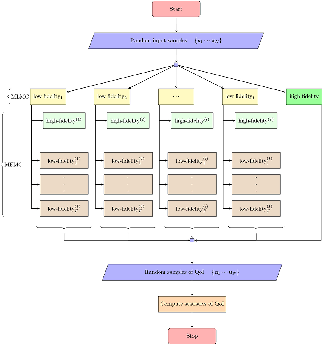
Figure 1. Outline of the (MFML-MC) method described in section 4. The low-fidelity_i (yellow color) denotes low-fidelity model i (i = 1, 2, … I) in MLMC setup. The low-fidelity${\text{low-fidelity}}_f^{(i)}$ (brown color) denotes low-fidelity f in MFMC method formulated in the ith MLMC setup. QoI denotes the quantity of interest or outputs of interest.

The first step of MFML-MC method is to formulate a sequence of POD approximations of the QoI u and utilize these sequence as low-fidelity models [v₁, …, v_I] in MLMC framework. More precisely, in this approach, v_i is ith level POD approximation of u and is computed from least-squares reconstruction method defined as

$\begin{array}{ll}\text{u}\approx {\text{v}}_i={\text{U}}_u^{r_i}\tilde{\text{u}}={\text{U}}_u^{r_i}({{\text{U}}_u^{r_i}}^{\top }\text{u})& (15)\end{array}$

where $\tilde{\text{u}}\in {ℝ}^{r_i}$ is the reduced representation of u, ${\text{U}}_u^{r_i}\in {{R}}^{m\times r_i}$ is the orthonormal matrix containing r_i orthonormal basis vectors in its columns. The optimal orthonormal basis vectors are computed from the singular value decomposition (SVD) of the snapshot matrix ${\text{X}}_u=\left({({\text{u}}_1\dots {\text{u}}_T)}^1\dots {({\text{u}}_1\dots {\text{u}}_T)}^L\right)$, where T denotes the number of time steps and L denotes the number of training samples corresponding to different realizations of the stochastic input parameters. The SVD of X_u is expressed as (Kani and Elsheikh, 2018)

$\begin{array}{ll}{\text{X}}_u={\text{U}}_u{\Sigma }_u{\text{W}}_u& (16)\end{array}$

where ${\text{U}}_u\in {ℝ}^{m\times m}$ is the left singular matrix, (σ₁ > σ₂ > σ₃ > … σ_m ≥ 0) are the singular values of the snapshot matrix X_u. The associated error termed as least–squares errors in approximating u by v_i using only r_i basis vectors is given by (Berkooz et al., 1993; Lucia et al., 2004)

$\begin{array}{ll}{\epsilon }_i=\parallel \text{u}-{\text{v}}_i{\parallel }_2={\displaystyle \sum _{j=r_i+1}^m}{\sigma }_j& (17)\end{array}$

Please note that the dimension m of the basis vector in U_u is much smaller than n (the number of grid points). Hence, for a large scale UQ problems where m≪n, we can easily form many levels with smaller ε_i in this MLMC framework in comparison to standard MLMC method. Moreover, v_I can be obtained by using less number of basis vectors (r_I ≈ m with ε_I ≈ 0) in comparison to standard MLMC method with a sequence of Galerkin projection based ROMs.

The second step of MFML-MC method is to compute the reduced representation of Y_i over all levels in MLMC framework (see Equation 9). The reduced representation of Y_i is expressed as

$\begin{array}{ll}{\tilde{\text{Y}}}_i={{\text{U}}_{Y_i}^{q_i}}^{\top }{\text{Y}}_i& (18)\end{array}$

where ${\tilde{\text{Y}}}_i\in {ℝ}^{q_i}$ is the reduced representation of Y_i, ${\text{U}}_{Y_i}^{q_i}\in {{R}}^{m\times q_i}$ is the orthonormal matrix containing q_i orthonormal basis vectors in its columns. The optimal orthonormal basis matrix ${\text{U}}_{Y_i}^{q_i}$ is computed from the singular value decomposition (SVD) of the snapshot matrix ${\text{X}}_{Y_i}=\left({({\text{Y}}_{i_1}\dots {\text{Y}}_{i_T})}^1\dots {({\text{Y}}_{i_1}\dots {\text{Y}}_{i_T})}^L\right)$, where Y_ij = v_i+1j − v_ij (i = 0 … I − 1) and Y_Ij = u_j − v_Ij for all j = 1, …, T. Since, Y_i is computed from the difference between two consecutive levels of POD based approximations v_i+1 and v_i, i.e., Y_i = v_i+1 − v_i, the least–squares error in approximating Y_i by $({\text{U}}_{Y_i}^{q_i}{\tilde{\text{Y}}}_i)$ is equivalent to the difference of two consecutive level ε (see Equation 17) which is expressed as $\Delta {\epsilon }_i={\epsilon }_i-{\epsilon }_{i+1}=\sum _{j=r_i+1}^{r_{i+1}}{\sigma }_j$.

Now the MLMC estimator (see Equation 11) for the expected value of u is expressed as

$\begin{array}{ll}𝔼\left[\text{u}\right]={\displaystyle \sum _{i=0}^I}𝔼\left[{\text{Y}}_i\right]\approx {\displaystyle \sum _{i=0}^I}{\text{U}}_{Y_i}^{q_i}𝔼[{\tilde{\text{Y}}}_i]={\widehat{\text{u}}}^{ml}={\displaystyle \sum _{i=0}^I}{\widehat{\text{Y}}}_i={\displaystyle \sum _{i=0}^I}{\text{U}}_{Y_i}^{q_i}{\widehat{\tilde{\text{Y}}}}_i& (19)\end{array}$

The third step of MFML-MC method is to set r_i for all i = 1 … I. In this framework, we set r_i = i. Now, Δε_i = σ_i and therefore, we expect Y_i to be attracted to a certain low dimensional subspace of dimension q_i = Δr_i = (r_i+1 − r_i) = 1 over all the levels.

In the fourth step, we extend the Multi-Level Multi-Fidelity method introduced in Geraci et al. (2015) by adopting multi-fidelity approach (see Equation 8) on every level of MLMC framework to derive an unbiased estimator of $𝔼[{\tilde{\text{Y}}}_i]$ in Equation (19) that takes the form

$\begin{array}{ll}{\widehat{\tilde{\text{Y}}}}_i^{mf}={\widehat{\tilde{\text{Y}}}}_i+{\beta }_i^1({\widehat{\tilde{\text{Y}}}}_i^1-{\widehat{\tilde{\text{Y}}}}_i)+{\displaystyle \sum _{f=2}^{F_i}}{\beta }_i^f({\widehat{\tilde{\text{Y}}}}_i^f-{\widehat{\tilde{\text{Y}}}}_i^{f-1})& (20)\end{array}$

where ${\tilde{\text{Y}}}_i^1\dots {\tilde{\text{Y}}}_i^{F_i}$ are auxiliary random variables obtained from F_i number of level specific low-fidelity models of ${\tilde{\text{Y}}}_i$, ${\widehat{\tilde{\text{Y}}}}_i^f$ estimates the expectation $𝔼[{\tilde{\text{Y}}}_i^f]$ using $M_i^f$ samples of ${\tilde{\text{Y}}}_i^f$ for all f = 1 … F_i, and ${\beta }_i^1\dots {\beta }_i^{F_i}\in ℝ$ are the coefficients on level i, i = 0 … I. In this paper, we set F_i = 1 for all i = 0 … I. Next, we use the optimization problem formulated in Peherstorfer et al. (2016) to select optimal values $M_{\mathrm{\text{HF}}}^{*}$, $M_i^{1^{*}}$ such that the mean square error of the MFML-MC estimator ${\widehat{\tilde{\text{Y}}}}_i^{mf}$ on every level is lower than the Monte Carlo estimator ${\widehat{\tilde{\text{Y}}}}_i$ for the same computational budget.

Now, the MFML-MC estimator for the expected value of u (see Equation 19) is expressed as

$\begin{array}{ll}𝔼\left[\text{u}\right]\approx {\widehat{\text{u}}}^{ml}={\displaystyle \sum _{i=0}^I}{\widehat{\text{Y}}}_i\approx {\displaystyle \sum _{i=0}^I}{\text{U}}_{Y_i}^{q_i}{\widehat{\tilde{\text{Y}}}}_i^{mf}& (21)\end{array}$

In the fifth step, we utilize a data-driven approach to derive a level specific low-fidelity model ${\tilde{\text{Y}}}_i^1$ in the MFMC setup. In this data-driven approach, we first consider a discrete nonlinear dynamical system on every level (i = 0 … I) that takes the form

$\begin{array}{ll}{\tilde{\text{Y}}}_i^1(t+1)={\tilde{\text{Y}}}_i^1(t)+{\text{F}}_i(\text{x},{\tilde{\text{Y}}}_i^1(t)),& (22)\end{array}$

where ${\text{F}}_i(\text{x},{\tilde{\text{Y}}}_i^1(t))$ is the nonlinear term utilized to update ${\tilde{\text{Y}}}_i^1(t+1)$ on level i for all i = 0 … I (Nagoor Kani and Elsheikh, 2017). Next, we use GBTR (Friedman, 2001) on every level to approximate ${\text{F}}_i(\text{x},{\tilde{\text{Y}}}_i^1(t))$. We use $(\text{x},{\tilde{\text{Y}}}_i^1(t))$ as an input to GBTR and compute ${\text{F}}_i(\text{x},{\tilde{\text{Y}}}_i^1(t))$ as an output. We fit GBTRs using the same training samples $\left({({\text{Y}}_{i_1}\dots {\text{Y}}_{i_T})}^1\dots {({\text{Y}}_{i_1}\dots {\text{Y}}_{i_T})}^L\right)$ utilized in the second step.

5. Numerical Experiments

In this section, we present numerical results to evaluate the performance of MFML-MC method. The numerical results are based on two UQ tasks involving two-phase flow in the heterogeneous porous media domain. The two test cases are quarter five spot problem and the uniform flow problem with the uncertainties in the permeability field (Kani and Elsheikh, 2018). In section 5.1, we describe high-fidelity model setup, in section 5.2, we describe low-fidelity model setup in order to formulate MFML-MC framework, in section 5.3, we describe MLMC with Galerkin-POD ROMs setup, and in section 5.4, we define a set of error metrics that we utilize to compare MFML-MC method with standard MC method that uses either high-fidelity model or low-fidelity model. In section 5.5, we provide the results for quarter five spot problem and in section 5.6, we provide the results for uniform flow problem.

5.1. High-Fidelity Model Setup

We consider two-phase flow of oil and water in a two dimensional porous media domain [0 1] × [0 1] where water is injected to displace the residual oil. We consider Equation (3) as a high-fidelity model to describe the flow behavior of oil and water. We define the relative permeability based on Corey's model $k_{rw}(s)={s^{*}}^2$, $k_{ro}={(1-s^{*})}^2$, where $s^{*}=(s-s_{wc})/(1-s_{or}-s_{wc})$, s_wc is the irreducible water saturation and s_or is the residual oil saturation (Aarnes et al., 2007). We set s_wc = 0.2, s_or = 0.2, and initial water saturation to s_wc(0.2). We set the porosity field in the porous media domain to a constant value of 0.2. We set viscosity ratio of water and oil to 0.2. We consider uncertainties from the permeability field and assumed to be modeled as a log-normal distribution function with zero mean and exponential covariance that takes the form

$\begin{array}{ll}ℂov={\sigma }_k^{2}exp\left[-\frac{|x_1-x_2|}{{\iota }_k}\right]& (23)\end{array}$

where ${\sigma }_k^2$ is the variance, ι_k is the correlation length. We set ${\sigma }_k^2$ to 1 and ι_k to 0.1. Sample realizations of log-permeability values are displayed in Figure 2.

FIGURE 2

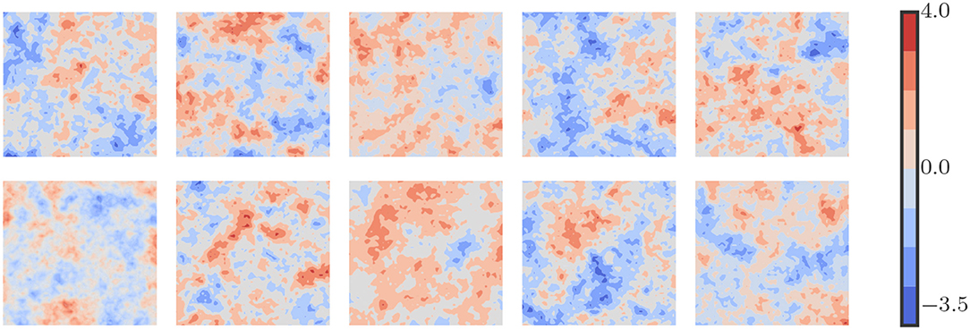
Figure 2. Sample plots of log-permeability field. Uncertain permeability field is modeled from a log-normal distribution function with zero mean and exponential covariance.

As mentioned in section 2, we use sequential formulation to solve Equation (3) for pressure and water saturation (Aarnes et al., 2007). We first generate a uniform mesh of 96 × 96 blocks in a spatial domain. We use finite volume method with two point flux approximation (Aarnes et al., 2007) to solve for pressure and an upwind finite-volume method with an implicit backward Euler method combined with Newton-Raphson iterative method to solve for saturation. We set time step size to 0.015 and we solve Equation (3) for 200 time steps. We solve pressure and update velocity field at every 8th time step as pressure field changes much slower than saturation field over time. Time is measured by a non dimensional unit called pore volumes injected (PVI) (Ibrahima, 2016).

As defined in section 2, QoI is u ∈ ℝ^m, where u_i = y_s(x_i, y_i), i = 1 … m≪n at specific time steps. The first moment estimate of u(t) at specific time steps are the desired statistic. The interested grid points ((x_i, y_i) i = 1 … m) are 6 × 6 grid points (m = 36) uniformly selected from the 96 × 96 spatial domain. The interested time steps are t = 10, 20, …, 200. We solve Equation (3) for 25,000 random realizations of the permeability field and use Monte Carlo method to estimate the statistics of u (Ibrahima, 2016).

5.2. Low-Fidelity Model Setup

We first compute the optimal POD bases matrices U_u and U_Yi for all i = 0 … I. We compute the POD matrices from the SVD of the snapshot matrices X_u, X_Yi, i = 0 … I. We built the snapshot matrices from 10 random samples of high-fidelity model solution data. In order to select the 10 random high-fidelity models to build snapshot matrices, we use K-means clustering algorithm to cluster 25,000 random permeability realizations into 10 clusters (Ghasemi, 2015). Then, we solve the high-fidelity model for a single permeability realization from each cluster.

Following that, the obtained matrix U_u is utilized to build a sequence of POD approximations of u (as detailed in the section 4) from the collected training data. Then the matrix ${\text{U}}_{Y_i}^{q_i}$ is utilized to compute training samples of ${\tilde{\text{Y}}}_i$ (the reduced representation of Y_i) for all i = 0 … I. We set I = 18, r_i = i, and therefore q_i = 1 as already mentioned in section 4.

Next, we build a level specific GBTR on every level (i = 0 … I) to estimate F_i and utilize the estimated F_i in Equation (22) to compute ${\tilde{\text{Y}}}_i^1(t+1)$. We use Scikit-learn (Pedregosa et al., 2011) a machine learning python package to implement the GBTRs. We use the training samples of ${\tilde{\text{Y}}}_i$ to fit the level specific GBTR.

5.3. Standard MLMC With POD-Galerkin ROMs Setup

We first compute optimal POD basis vectors for the pressure and saturation solution vectors from the SVD of the corresponding snapshot matrices. We built the snapshot matrices from the solution vectors (pressure and saturation) collected from the solutions of the high-fidelity model for 45 random realizations of the permeability field. We then built low-fidelity ROM models of different dimensions via Galerkin projection of the discretized system of the high-fidelity model Equation (3) on to the POD space spanned by the POD basis vectors.

Following that one can obtain MLMC framework using Galerkin projection POD ROMs as low-fidelity models. However, in the two numerical test cases namely, the quarter five spot problem (5.5), and the uniform flow problem (5.6), we obtained accurate and stable POD results only when the dimensions of the POD-Galerkin ROMs were on the order of magnitude nearly equivalent to the dimension of the high-fidelity state variable (Xiao et al., 2017; Kani and Elsheikh, 2018). Hence, the computational cost to obtain the QoI from the POD-Galerkin ROM is more than the computational cost to obtain the QoI from the high-fidelity model for a single realization. Therefore, it was infeasible to derive an effective MLMC framework with a hierarchy of low-fidelity models based on standard POD ROMs. This is expected because the governing equations of the flow problem Equation (3) has nonpolynomial nonlinearity and is well known issue in reduced order modeling for multi-phase subsurface flow problems (Chaturantabut and Sorensen, 2011; He et al., 2011; Jansen and Durlofsky, 2017; Kani and Elsheikh, 2018). We also note that we conducted extensive study on reduced order modeling for these two problems in Kani and Elsheikh (2018) and we obtained inaccurate and unstable results when using POD ROMs. At this point, we request the readers to refer figures included in the numerical results section of Kani and Elsheikh (2018), where some of the standard POD ROM unstable results are displayed. Hence, we have not included the comparison of MFML-MC method with MLMC method based on standard POD ROMs as low-fidelity models.

5.4. Evaluation Metrics

We evaluate the performance of MFML-MC method using two time specific error metrics defined by

$\begin{array}{l}{\widehat{e}}_t^{\text{bias}}=\frac{1}{N_{\text{e}}}{\displaystyle \sum _{j=1}^{N_{\text{e}}}}\parallel {\widehat{\text{u}}}_t^{\text{ref}}-{\widehat{\text{u}}}_t^{(j)}{\parallel }_2^2\\ {\widehat{e}}_t^{ϵ}=\frac{1}{N_{\text{e}}}{\displaystyle \sum _{j=1}^{N_{\text{e}}}}\text{𝕍}\text{ar}({\widehat{\text{u}}}_t^{(j)})& (24)\end{array}$

where N_e is the number of runs utilized to estimate the errors, ${\widehat{\text{u}}}_t^{\mathrm{\text{ref}}}$ is the reference result of 𝔼[u_t] obtained from Monte Carlo estimate ${\widehat{\text{u}}}_t^{\mathrm{\text{(MC)}}}$ computed with N = 25, 000 high-fidelity model samples. ${\widehat{\text{u}}}_t^{(j)}$ is the approximation of 𝔼[u_t] that can be obtained from various estimators including Monte Carlo estimate that uses only high-fidelity model, Monte Carlo estimate that uses only low-fidelity model, and the MFML-MC estimator. We note that, ${\widehat{\text{u}}}_t^{(j)}$ is obtained for a fixed computational budget p. The computational budget is measured in terms of the cost required to run p number of MC realizations that uses only high-fidelity model. We also note that, ${\widehat{\text{u}}}_t^{(j)}$ is evaluated from a different set of independent samples for set j = 1 … N_e.

Additionally, we utilize two global error metrics defined as

$\begin{array}{l}{\widehat{e}}^{\text{bias}}=\frac{1}{N_{\text{e}}}{\displaystyle \sum _{j=1}^{N_{\text{e}}}}{\displaystyle \underset{t=1}{\overset{T}{max}}}\parallel {\widehat{\text{u}}}_t^{\text{ref}}-{\widehat{\text{u}}}_t^{(j)}{\parallel }_2^2\\ {\widehat{e}}^{ϵ}=\frac{1}{N_{\text{e}}}{\displaystyle \sum _{j=1}^{N_{\text{e}}}}{\displaystyle \underset{t=1}{\overset{T}{max}}}𝕍\text{ar}({\widehat{\text{u}}}_t^{(j)})& (25)\end{array}$

where all the time snapshots of u are used. We set N_e = 15 to evaluate the two time specific error metrics and the two global error metrics.

5.5. Numerical Test Case 1

Test case 1 is two dimensional quart-five spot problem where water is injected in the lower left corner (0, 0) of the porous media domain to produce oil and water in the top right corner (1, 1) (Kani and Elsheikh, 2018). We set q defined in the saturation equation (Equation 3) to 0.05 at (0, 0) and −0.05 at (1, 1). We set no flux boundary condition in all the four sides of the porous media domain. The left panel of Figure 3 displays the quart-five spot problem set up and the right panel of Figure 3 displays the decay of the singular values of the snapshot matrix X_u.

FIGURE 3

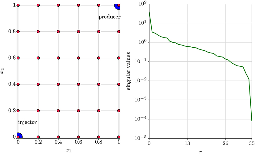
Figure 3. Test case 1. (Left) Two dimensional quart-five spot problem set-up where water is injected in the lower left corner (blue dot). Oil is displaced and produced with water in the upper right corner (blue dot). The red dots denotes spatial locations in the porous media domain where the statistics of the QoI u are investigated. (Right) Decay of singular values of the snapshot matrix X_u.

Figure 4 shows the results for the estimation of 𝔼[u_t] (first moment of u) obtained from the reference result (MC estimate with 25,000 samples) and from various MC estimators. In Figure 4, MC estimator that uses only high-fidelity model is denoted as MC-HF and that uses only low-fidelity model is denoted as MC-LF. In Figure 4, results shown in the top row are obtained at time = 0.3 PVI and results shown in the bottom row are obtained at time = 0.8 PVI. As shown in Figure 4, the estimation of 𝔼[u_t] obtained from MC-LF deviates significantly from the reference result. This clearly shows that utilizing only low-fidelity model in MC framework resultant in biased estimation with respect to the reference result. Furthermore, Figure 4 shows that the estimation of 𝔼[u_t] obtained from MFML-MC estimator is almost indistinguishable from the reference result. This result confirm that combining higher number of low-fidelity model realizations with the high-fidelity model in MFML-MC framework can improve the estimator of the first moment of the saturation field.

FIGURE 4

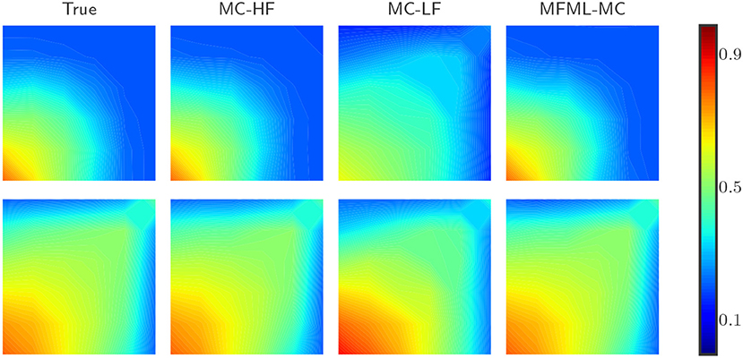
Figure 4. Test case 1: Comparison of estimation of 𝔼[u_t] (mean water saturation field at 6 × 6 spatial grid) for a fixed computational budget p = 100, where p is the number of MC realizations that uses only high-fidelity model. (Top Row) Estimation of 𝔼[u_t] at time t = 0.3 PVI. (Bottom Row) Estimation of E[u_t] at time t = 0.8 PVI.

Figure 5 reports the comparison of ${\widehat{e}}_t^{\mathrm{\text{bias}}}$ and ${\widehat{e}}_t^{ϵ}$ (see Equation 24) obtained from various estimators. The left of Figure 5 reports ${\widehat{e}}_t^{\mathrm{\text{bias}}}$ and the right of Figure 5 reports ${\widehat{e}}_t^{ϵ}$ as a function of computational budget p = [1, 2, 3, 4, 5] × 10², where p is the number of MC-HF realizations. The results of ${\widehat{e}}_t^{\mathrm{\text{bias}}}$ from Figure 5 shows that Monte Carlo estimator that uses MC-LF is a biased estimator of the mean QoI value. The results of MFML-MC estimator displayed in left of Figure 5 confirm that the MFML-MC estimator is an unbiased estimator of the expectation. This shows that despite the low-fidelity model is a poor approximation of the high-fidelity model, the error of the MFML-MC estimator can be significantly reduced if the low-fidelity model is combined with the high-fidelity. The right of Figure 5 shows that the variance of the MFML-MC and MC-LF estimators are at least an order of magnitude less when compared to MC-HF. Nevertheless, while MC-LF is a biased estimator as shown in left of Figure 5, MFML-MC estimator that uses the low-fidelity model in combination with the high-fidelity model is an unbiased estimator of the expectation.

FIGURE 5

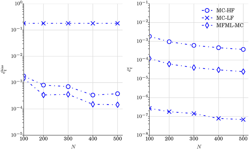
Figure 5. Test case 1: Plot of ${\widehat{e}}_t^{\mathrm{\text{bias}}}$, and ${\widehat{e}}_t^{ϵ}$ (Equation 24) for the estimation of 𝔼[u_t] (water saturation field at 6 × 6 spatial grid) obtained from various estimators. ${\widehat{e}}_t^{\mathrm{\text{bias}}}$ and ${\widehat{e}}_t^{ϵ}$ are shown as a function of computational budget p = [1, 2, 3, 4, 5] × 10², where p is the number of MC realizations N that uses only high-fidelity model. (Left) ${\widehat{e}}_t^{\mathrm{\text{bias}}}$ at time t = 0.3 PVI. (Right) ${\widehat{e}}_t^{ϵ}$ at time t = 0.3 PVI.

Figure 6 reports the comparison of ${\widehat{e}}^{\text{bias}}$ and ${\widehat{e}}^{ϵ}$ (see Equation 25) obtained from various estimators. We can clearly observe the trend of ${\widehat{e}}^{\text{bias}}$, and ${\widehat{e}}^{ϵ}$ in Figure 6 are similar to the one observed in Figure 5 which confirms that MFML-MC method leads to variance reduction with unbiased estimation at all time steps.

FIGURE 6

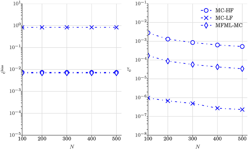
Figure 6. Test case 1: Plot of ${\widehat{e}}^{\text{bias}}$ and ${\widehat{e}}^{ϵ}$ (Equation 25) estimation of 𝔼[u] (water saturation field at 6 × 6 spatial grid) obtained from various estimators. ${\widehat{e}}^{\text{bias}}$ and ${\widehat{e}}^{ϵ}$ are shown as a function of computational budget p = [1, 2, 3, 4, 5] × 10², where p is the number of MC realizations N that uses only high-fidelity model.

Table 1 compare the speedup factors of MFML-MC method with respect to the Monte Carlo estimator that uses the high-fidelity model only. In Table 1, MFML-MC achieves a speedup with respect to MC-HF that range from 8 up to 15 for the same specific ϵ.

TABLE 1

Table 1. Performance chart of MFML-MC estimator for test case 1.

5.6. Numerical Test Case 2

Test case 2 is a two dimensional uniform flow problem where water is injected from the left side of the porous media domain to produce oil and water from the right side. We set no flow boundary conditions in the remaining two sides (top and bottom) of the domain. We set inflow rate to 0.08 and outflow rate to 0.08 due to incompressibility constraint set in the problem (Kani and Elsheikh, 2018). The left panel of Figure 7 displays uniform flow problem set up and the right panel of Figure 7 displays the decay of the singular values of the snapshot matrix X_u.

FIGURE 7

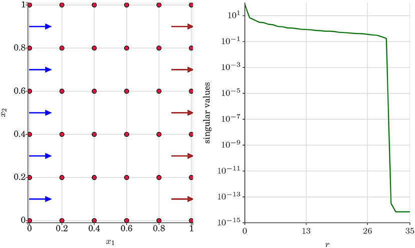
Figure 7. Test case 2: (Left) Uniform flow problem set up where water is injected from the left side denoted by blue arrows. Oil and water are produced from the right side denoted by brown arrows. The red dots denotes the spatial locations of the porous media domain where the statistics of the QoI u are investigated. (Right) Decay of singular values of the snapshot matrix X_u.

Figure 8 shows the results for the first moment of the saturation field (u) obtained from the reference result (MC estimate with 25000 samples) and from various MC estimators. The display settings defined in Figure 8 are the same as the one defined in Figure 4. In Figure 8, we can see that the results obtained from MFML-MC method are almost indistinguishable from the reference results whereas MC-LF yields extremely inaccurate results.

FIGURE 8

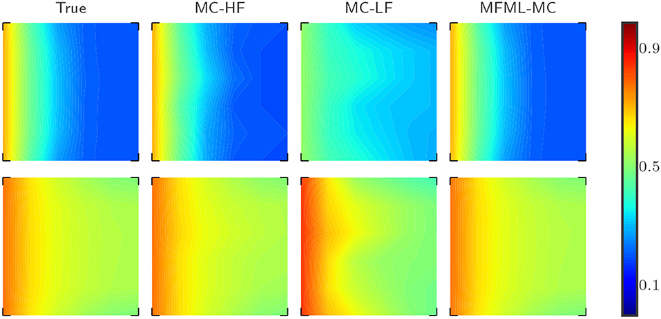
Figure 8. Test case 2: Comparison of estimation of 𝔼[u_t] (mean water saturation field at 6 × 6 spatial grid) for a fixed computational budget p = 100, where p is the number of MC realizations that uses only high-fidelity model. (Top Row) Estimation of 𝔼[u_t] at time t = 0.3 PVI. (Bottom Row) Estimation of 𝔼[u_t] at time t = 0.8 PVI.

Figure 9 reports the comparison of ${\widehat{e}}_t^{\mathrm{\text{bias}}}$ and ${\widehat{e}}_t^{ϵ}$ (see Equation 24) obtained from various estimators. The variance reduction can be clearly observed in Figure 9 and the trend of Figure 9 is similar to the one observed in Figure 5 (Test case 1). The results of Figure 9 again confirm that combining the high-fidelity model with the low-fidelity model leads to a variance reduction. Please note that a similar confirmation was observed in Figure 5.

FIGURE 9

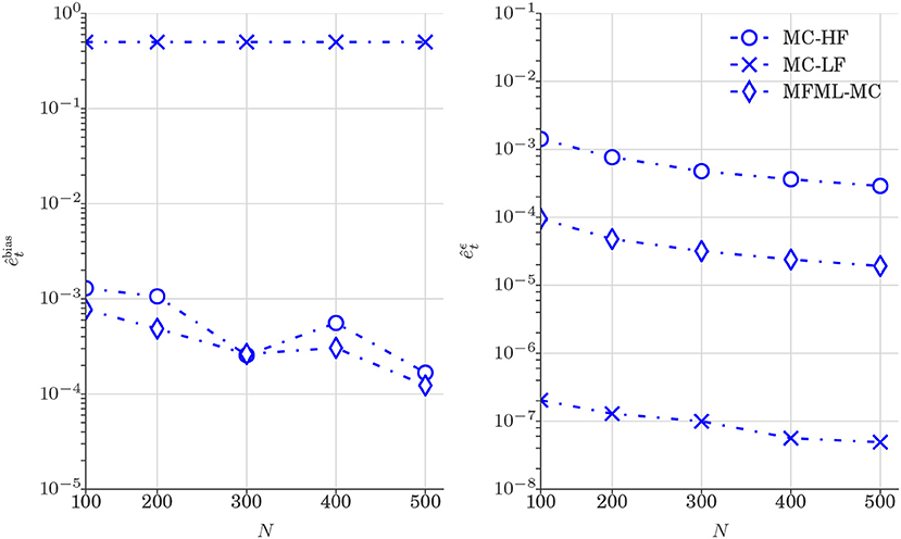
Figure 9. Test case 2: Plot of ${\widehat{e}}_t^{\mathrm{\text{bias}}}$ and ${\widehat{e}}_t^{ϵ}$ (Equation 24) for the estimation of 𝔼[u_t] (water saturation field at 6 × 6 spatial grid) obtained from various estimators. ${\widehat{e}}_t^{\mathrm{\text{bias}}}$ and ${\widehat{e}}_t^{ϵ}$ are shown as a function of computational budget p = [1, 2, 3, 4, 5] × 10², where p is the number of MC realizations N that uses only high-fidelity model. (Left) ${\widehat{e}}_t^{\mathrm{\text{bias}}}$ at time t = 0.3 PVI. (Right) ${\widehat{e}}_t^{ϵ}$ at time t = 0.3 PVI.

Figure 10 reports the comparison of ${\widehat{e}}^{\text{bias}}$ and ${\widehat{e}}^{ϵ}$ (see Equation 25) obtained from various estimators. As observed in Figure 6, the results displayed in Figure 9 shows that MFML-MC method leads to variance reduction with unbiased estimation.

FIGURE 10

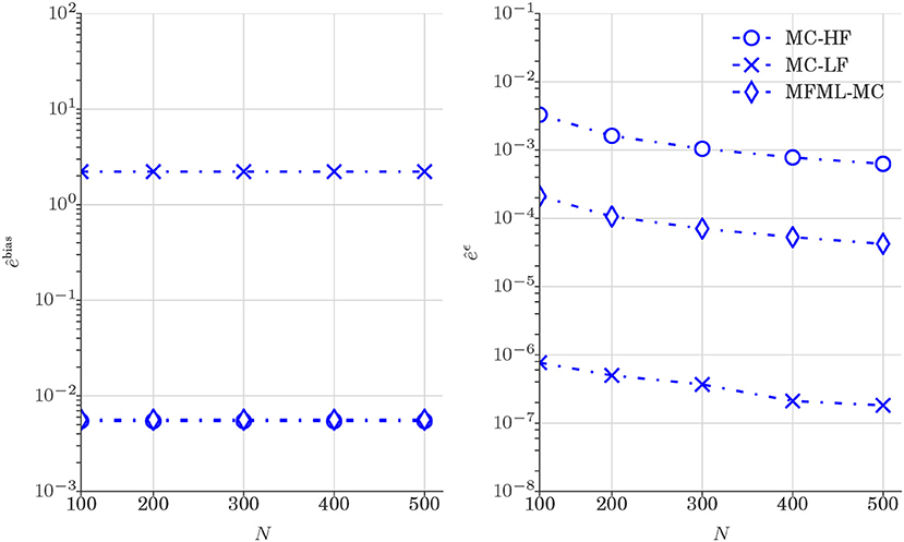
Figure 10. Test case 2: Plot of ${\widehat{e}}^{\text{bias}}$ and ${\widehat{e}}^{ϵ}$ (Equation 25) for the estimation of 𝔼[u] (water saturation field at 6 × 6 spatial grid) obtained from various estimators. ${\widehat{e}}^{\text{bias}}$ and ${\widehat{e}}^{ϵ}$ are shown as a function of computational budget p = [1, 2, 3, 4, 5] × 10², where p is the number of MC realizations N that uses only high-fidelity model.

Table 2 compare the speedup factors of MFML-MC method with respect to the MC method that uses the high-fidelity model only. In Table 2, MFML-MC achieves a speedup with respect to MC-HF that range from 10 up to 19 at a specific ϵ.

TABLE 2

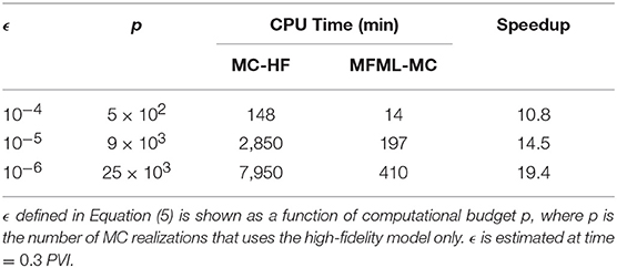
Table 2. Performance chart of MFML-MC estimator for test case 2.

6. Conclusion

In this paper, we proposed a MFML-MC method combining the features of both the MFMC method and the MLMC method. In MFML-MC method, we formulated MLMC framework with a sequence of POD approximations of high-fidelity model outputs. Furthermore, in MFML-MC method, we formulated a MFMC setup on every level of MLMC framework in order to compute an unbiased statistical estimation. Finally, we utilized GBTR in the MFMC setup to formulate a level specific low-fidelity model.

We applied MFML-MC method on two uncertainty quantification problems involving two-phase flows in random heterogeneous porous media where standard MLMC method with POD-Galerkin ROMs is ineffective. The uncertain permeability field is modeled from log-normal distribution function with exponential covariance function. Estimate of the first statistical moments of the water saturation at uniformly selected spatial grid points over a specific instant in time are calculated by MFML-MC, MC-HF, and MC-LF methods. Comparisons between MFML-MC and MC-LF suggested that MC-LF as a biased estimator and MFML-MC estimator as an unbiased estimator of the expectation. Comparisons between the MFML-MC and MC-HF computing times showed speedups of MFML-MC with respect to MC-HF that ranged from 8 up to 19 at equivalent accuracy.

Future work should consider the extension of MFML-MC method by utilizing two or more level specific low-fidelity models in the MFMC setup. In addition, it will also be interest to use MFML-MC method for history matching (Elsheikh et al., 2012, 2013), where we aim to minimize the mismatch between field observation data and the one computed from the high-fidelity model simulations by adjusting the geological model parameters. Future work should also verify the applicability of MFML-MC method for large-scale realistic problems with many wells and time varying injection rates by which the potential of MFML-MC method in speeding up a realistic Monte Carlo simulation can be magnified.

Author Contributions

NJ developed the algorithm, coded the algorithm in python and obtained the results, and wrote the manuscript. AE is the Ph.D. supervisor of NJ. NJ did this paper under the guidance of AE.

Conflict of Interest Statement

The authors declare that the research was conducted in the absence of any commercial or financial relationships that could be construed as a potential conflict of interest.

References

Aarnes, J. E., Gimse, T., and Lie, K. A. (2007). “An introduction to the numerics of flow in porous media using Matlab,” in Geometric Modelling, Numerical Simulation, and Optimization (Oslo: Springer), 265–306.

Google Scholar

Abdulle, A., Barth, A., and Schwab, C. (2013). Multilevel monte carlo methods for stochastic elliptic multiscale pdes. Multisc. Model. Simulat. 11, 1033–1070. doi: 10.1137/120894725

CrossRef Full Text | Google Scholar

Antoulas, A. C., Sorensen, D. C., and Gugercin, S. (2001). A survey of model reduction methods for large-scale systems. Contemp. Math. 280, 193–220. doi: 10.1090/conm/280/04630

CrossRef Full Text | Google Scholar

Babuška, I., Nobile, F., and Tempone, R. (2007). A stochastic collocation method for elliptic partial differential equations with random input data. SIAM J. Numer. Anal. 45, 1005–1034. doi: 10.1137/050645142

CrossRef Full Text | Google Scholar

Barth, A., Schwab, C., and Zollinger, N. (2011). Multi-level monte carlo finite element method for elliptic pdes with stochastic coefficients. Numerische Math. 119, 123–161. doi: 10.1007/s00211-011-0377-0

CrossRef Full Text | Google Scholar

Bastian, P. (1999). Numerical computation of multiphase flow in porous media. (Ph.D. thesis). Habilitationsschrift Univeristät Kiel, Berlin, Germany.

Google Scholar

Berkooz, G., Holmes, P., and Lumley, J. L. (1993). The proper orthogonal decomposition in the analysis of turbulent flows. Annu. Rev. Fluid Mech. 25, 539–575. doi: 10.1146/annurev.fl.25.010193.002543

CrossRef Full Text | Google Scholar

Bui-Thanh, T., Willcox, K., Ghattas, O., and Waanders, B. V. (2007). Goal-oriented, model-constrained optimization for reduction of large-scale systems. J. Comput. Phys. 224, 880–896. doi: 10.1016/j.jcp.2006.10.026

CrossRef Full Text | Google Scholar

Chaturantabut, S., and Sorensen, D. C. (2011). Application of POD and DEIM on dimension reduction of non-linear miscible viscous fingering in porous media. Math. Comput. Modell. Dyn. Syst. 17, 337–353. doi: 10.1080/13873954.2011.547660

CrossRef Full Text | Google Scholar

Chen, Z., Huan, G., and Ma, Y. (2006). Computational Methods for Multiphase Flows in Porous Media. Dallas, TX: SIAM.

Google Scholar

Cliffe, K. A., Giles, M. B., Scheichl, R., and Teckentrup, A. L. (2011). Multilevel monte carlo methods and applications to elliptic pdes with random coefficients. Comput. Visualizat. Sci. 14:3. doi: 10.1007/s00791-011-0160-x

CrossRef Full Text | Google Scholar

Codina, F. V., Ngoc, N. C., Giles, M. B., and Peraire, J. (2015). A model and variance reduction method for computing statistical outputs of stochastic elliptic partial differential equations. J. Comput. Phys. 297, 700–720. doi: 10.1016/j.jcp.2015.05.041

CrossRef Full Text | Google Scholar

Codina, F. V., Ngoc, N. C., Giles, M. B., and Peraire, J. (2016). An empirical interpolation and model-variance reduction method for computing statistical outputs of parametrized stochastic partial differential equations. SIAM/ASA J. Uncertain. Quantificat. 4, 244–265. doi: 10.1137/15M1016783

CrossRef Full Text | Google Scholar

Doostan, A., and Owhadi, H. (2011). A non-adapted sparse approximation of pdes with stochastic inputs. J. Comput. Phys. 230, 3015–3034. doi: 10.1016/j.jcp.2011.01.002

CrossRef Full Text | Google Scholar

Durlofsky, L. J., and Chen, Y. (2012). “Uncertainty quantification for subsurface flow problems using coarse-scale models,” in Numerical Analysis of Multiscale Problems, eds I. Graham, T. Hou, O. Lakkis, and R. Scheichl (Berlin: Springer), 163–202.

Google Scholar

Efendiev, Y., Iliev, O., and Kronsbein, C. (2013). Multilevel monte carlo methods using ensemble level mixed msfem for two-phase flow and transport simulations. Compu. Geosci. 17, 833–850. doi: 10.1007/s10596-013-9358-y

CrossRef Full Text | Google Scholar

Efendiev, Y., Jin, B., Michael, P., and Tan, X. (2015). Multilevel markov chain monte carlo method for high-contrast single-phase flow problems. Commun. Comput. Phys. 17, 259–286. doi: 10.4208/cicp.021013.260614a

CrossRef Full Text | Google Scholar

Elsakout, D., Christie, M., Lord, G., et al. (2015). “Multilevel markov chain monte carlo (mlmcmc) for uncertainty quantification,” in SPE North Africa Technical Conference and Exhibition (Cairo: Society of Petroleum Engineers).

Google Scholar

Elsheikh, A. H., Jackson, M., and Laforce, T. (2012). Bayesian reservoir history matching considering model and parameter uncertainties. Math. Geosci. 44, 515–543. doi: 10.1007/s11004-012-9397-2

CrossRef Full Text | Google Scholar

Elsheikh, A. H., Wheeler, M. F., and Hoteit, I. (2013). Nested sampling algorithm for subsurface flow model selection, uncertainty quantification, and nonlinear calibration. Water Resour. Res. 49, 8383–8399. doi: 10.1002/2012WR013406

CrossRef Full Text | Google Scholar

Fagerlund, F., Hellman, F., Målqvist, A., and Niemi, A. (2016). Multilevel monte carlo methods for computing failure probability of porous media flow systems. Adv. Water Resour. 94, 498–509. doi: 10.1016/j.advwatres.2016.06.007

CrossRef Full Text | Google Scholar

Frangos, M., Marzouk, Y., Willcox, K., and Waanders, B. V. (2010). Surrogate and Reduced-Order Modeling: A Comparison of Approaches for Large-Scale Statistical Inverse Problems. Alburquerque: John Wiley & Sons, Ltd.

Google Scholar

Friedman, J. H. (2001). Greedy function approximation: a gradient boosting machine. Ann. Stat. 29, 1189–1232. doi: 10.1214/aos/1013203451

CrossRef Full Text | Google Scholar

Geraci, G., Eldred, M., and Iaccarino, G. (2015). “A multifidelity control variate approach for the multilevel monte carlo technique,” in Center for Turbulence Research Annual Research Briefs (Alburquerque).

Google Scholar

Ghanem, R. G., and Spanos, P. D. (1991). “Stochastic finite element method: response statistics,” in Stochastic Finite Elements: A Spectral Approach (New York, NY: Springer), 101–119.

Google Scholar

Ghasemi, M. (2015). Model order reduction in porous media flow simulation and optimization. (Ph.D. thesis). Texas AM Univeristy, Austin, TX.

Google Scholar

Giles, M. B. (2008). Multilevel monte carlo path simulation. Operat. Res. 56, 607–617. doi: 10.1287/opre.1070.0496

CrossRef Full Text | Google Scholar

Giles, M. B. (2013). “Multilevel Monte Carlo methods,” in Monte Carlo and Quasi-Monte Carlo Methods 2012, eds J. Dick, F. Kuo, G. Peters, and I. Sloan (Berlin: Springer), 83–103.

Google Scholar

Giles, M. B. (2015). Multilevel monte carlo methods. Acta Numer. 24, 259–328. doi: 10.1017/S096249291500001X

CrossRef Full Text | Google Scholar

He, J. (2010). Enhanced linearized reduced-order models for subsurface flow simulation. (M.S. thesis). Stanford Univeristy, Stanford, CA.

Google Scholar

He, J., Sætrom, J., and Durlofsky, L. J. (2011). Enhanced linearized reduced-order models for subsurface flow simulation. J. Comput. Phys. 230, 8313–8341. doi: 10.1016/j.jcp.2011.06.007

CrossRef Full Text | Google Scholar

Heinrich, S. (2001). “Multilevel monte carlo methods,” in Large-Scale Scientific Computing, eds S. Margenov, J. Waśniewski, and P. Yalamov (Berlin; Heidelberg: Springer), 58–67.

Google Scholar

Ibrahima, F. (2016). Probability distribution methods for nonlinear transport in heterogenous porous media. (Ph.D. thesis). Stanford Univeristy, Stanford, CA.

Google Scholar

Jansen, J. D., and Durlofsky, L. J. (2017). Use of reduced-order models in well control optimization. Optimizat. Eng. 18, 105–132. doi: 10.1007/s11081-016-9313-6

CrossRef Full Text | Google Scholar

Kani, J. N., and Elsheikh, A. H. (2018). “Reduced-order modeling of subsurface multi-phase flow models using deep residual recurrent neural networks,” in Transport in Porous Media, eds Z. Zhang, J. Chi, S. Sun, and Z. Pan (Springer), 1–29.

Google Scholar

Kebaier, A. (2005). Statistical romberg extrapolation: a new variance reduction method and applications to option pricing. Ann. Appl. Probabil. 15, 2681–2705. doi: 10.1214/105051605000000511

CrossRef Full Text | Google Scholar

Lassila, T., Manzoni, A., Quarteroni, A., and Rozza, G. (2014). “Model order reduction in fluid dynamics: challenges and perspectives,” in Reduced Order Methods for Modeling and Computational Reduction, eds A. Quarteroni and G. Rozza (Cham: Springer), 235–273.

Google Scholar

Li, H., and Zhang, D. (2007). Probabilistic collocation method for flow in porous media: comparisons with other stochastic methods. Water Resour. Res. 43. doi: 10.1029/2006WR005673

CrossRef Full Text | Google Scholar

Lin, G., and Tartakovsky, A. M. (2009). An efficient, high-order probabilistic collocation method on sparse grids for three-dimensional flow and solute transport in randomly heterogeneous porous media. Adv. Water Resour. 32, 712–722. doi: 10.1016/j.advwatres.2008.09.003

CrossRef Full Text | Google Scholar

Lu, D., Zhang, G., Webster, C., and Barbier, C. (2016). An improved multilevel monte carlo method for estimating probability distribution functions in stochastic oil reservoir simulations. Water Resour. Res. 52, 9642–9660. doi: 10.1002/2016WR019475

CrossRef Full Text | Google Scholar

Lucia, D. J., Beran, P. S., and Silva, W. A. (2004). Reduced-order modeling: new approaches for computational physics. Prog. Aerospace Sci. 40, 51–117. doi: 10.1016/j.paerosci.2003.12.001

CrossRef Full Text | Google Scholar

Mishra, S., Schwab, C., and Šukys, J. (2012). Multi-level monte carlo finite volume methods for nonlinear systems of conservation laws in multi-dimensions. J. Comput. Phys. 231, 3365–3388. doi: 10.1016/j.jcp.2012.01.011

CrossRef Full Text | Google Scholar

Mishra, S., Schwab, C., and Šukys, J. (2016). Multi-level monte carlo finite volume methods for uncertainty quantification of acoustic wave propagation in random heterogeneous layered medium. J. Comput. Phys. 312, 192–217. doi: 10.1016/j.jcp.2016.02.014

CrossRef Full Text | Google Scholar

Müller, F., Jenny, P., and Meyer, D. W. (2013). Multilevel monte carlo for two phase flow and buckley–leverett transport in random heterogeneous porous media. J. Comput. Phys. 250, 685–702. doi: 10.1016/j.jcp.2013.03.023

CrossRef Full Text | Google Scholar

Nagoor Kani, J., and Elsheikh, A. H. (2017). DR-RNN: a deep residual recurrent neural network for model reduction. arxiv 1709.00939.

Google Scholar

Ng, L. W.-T. (2013). Multifidelity approaches for design under uncertainty. (Ph.D. thesis). Massachusetts: Massachusetts Institute of Technology.

Google Scholar

Pedregosa, F., Varoquaux, G., Gramfort, A., Michel, V., Thirion, B., Grisel, O., et al. (2011). Scikit-learn: machine learning in Python. J. Mach. Learn. Res. 12, 2825–2830.

Google Scholar

Peherstorfer, B., Willcox, K., and Gunzburger, M. (2016). Optimal model management for multifidelity monte carlo estimation. SIAM J. Sci. Comput. 38, A3163–A3194. doi: 10.1137/15M1046472

CrossRef Full Text | Google Scholar

Peherstorfer, B., Willcox, K., and Gunzburger, M. (2018). Survey of multifidelity methods in uncertainty propagation, inference, and optimization. SIAM Rev. 60, 550–591. doi: 10.1137/16M1082469

CrossRef Full Text | Google Scholar

Petvipusit, K. R., Elsheikh, A. H., Laforce, T. C., King, P. R., and Blunt, M. J. (2014). Robust optimisation of CO2 sequestration strategies under geological uncertainty using adaptive sparse grid surrogates. Comput. Geosci. 18, 763–778. doi: 10.1007/s10596-014-9425-z

CrossRef Full Text | Google Scholar

Stefanou, G. (2009). The stochastic finite element method: past, present and future. Comput. Methods Appl. Mech. Eng. 198, 1031–1051. doi: 10.1016/j.cma.2008.11.007

CrossRef Full Text | Google Scholar

Wang, Z., Akhtar, I., Borggaard, J., and Iliescu, T. (2012). Proper orthogonal decomposition closure models for turbulent flows: a numerical comparison. Comput. Methods Appl. Mech. Eng. 237, 10–26. doi: 10.1016/j.cma.2012.04.015

CrossRef Full Text | Google Scholar

Wang, Z., Xiao, D., Fang, F., Govindan, R., Pain, C. C., and Guo, Y. (2017). Model identification of reduced order fluid dynamics systems using deep learning. Int. J. Numer. Methods Fluids 86, 255–268. doi: 10.1002/fld.4416

CrossRef Full Text | Google Scholar

Xiao, D., Lin, Z., Fang, F., Pain, C. C., Navon, I. M., Salinas, P., et al. (2017). Non-intrusive reduced-order modeling for multiphase porous media flows using smolyak sparse grids. Int. J. Numer. Methods Fluids 83, 205–219. doi: 10.1002/fld.4263

CrossRef Full Text | Google Scholar