Exploring the Impacts of Seagrass on Coupled Marsh-Tidal Flat Morphodynamics

Intertidal coastal environments are prone to changes induced by sea level rise, increases in storminess, temperature, and anthropogenic disturbances. It is unclear how changes in external drivers may affect the dynamics of low energy coastal environments because their response is non-linear, and characterized by many thresholds and discontinuities. As such, process-based modeling of the ecogeomorphic processes underlying the dynamics of these ecosystems is useful, not only to predict their change through time, but also to generate new hypotheses and research questions. Here, we used a three-point dynamic model to investigate how seagrass might affect the behavior of coupled marsh-tidal flat systems. The model directly incorporates ecogeomorphological feedbacks among wind waves, salt marsh vegetation, allochthonous sediment loading, seagrasses and sea level rise. The model was applied to examine potential behaviors of salt marsh systems in the Virginia coastal bays. Differences due to the presence or absence of seagrass and stochastic vs. constant drivers lead to the emergence of complex behaviors in the coupled salt marsh-tidal flat system. In intertidal areas without seagrass, small tidal flats are unlikely to expand and provide enough sediment to the salt marshes to combat sea level rise. However, as the tidal flat expands, the concurrent increase in sediment supply due to wave-induced processes allows for the salt marsh to maintain pace with sea level at the expense of salt marsh extent. The presence of seagrass has two effects: (1) it decreases near bed shear stresses thus reducing the sediment flux to the salt marsh platform; (2) it reduces the wave energy acting on the salt marsh scarp, thus reducing boundary erosion. Model results indicate that the reductions in wave power and near bed shear stresses when seagrass is present provide an overall stabilizing effect on the coupled marsh-tidal flat system; but as water depth increases due to sea level rise or as external sediment supply increases, light conditions decline and the system reverts to that of a bare tidal flat.

Introduction

Much concern has been expressed recently regarding the susceptibility of salt marshes to the threat of sea level rise (SLR) owing to the critical ecosystem services they provide (Allen, 2000; Fagherazzi et al., 2004; Kirwan et al., 2016). The vertical accretion of a salt marsh is dependent on both organic sediment production and inorganic sediment supply (Allen, 1990). Organogenic sediment production is a function of local marsh characteristics, seasonal drivers and tidal range (Kirwan et al., 2008, 2009; Mudd et al., 2010; Kirwan and Mudd, 2012) whereas the availability of inorganic sediment to the marsh platform is dependent on transport of suspended sediments from the adjacent tidal flats and channels (Stumpf, 1983; Christiansen et al., 2000; Fagherazzi and Wiberg, 2009; Fagherazzi et al., 2013; Mariotti and Fagherazzi, 2013). Lateral erosion or accretion of the marsh platform depends directly on both inorganic sediment supply and the wave energy conditions at the bay-marsh boundary, both of which are influenced by the morphological characteristics of the adjacent tidal flats. Lateral erosion of the salt marsh edge can result in accumulation of inorganic sediment on the marsh platform(Chmura et al., 2001), thus linking the evolution of the salt marsh platform to the adjacent tidal flat.

While some studies have focused on anthropogenic influences and other geomorphological constraints, most tend to promote allochthonous sediment supply as the primary factor controlling whether salt marshes are prone to drowning or able to maintain pace with sea level rise (Fagherazzi et al., 2012). Moreover, recent work has shown that the horizontal extent of marshes is highly unstable with salt marshes either eroding or accreting depending on the relative size (and hence fetch) of the tidal flat to which they are coupled (Mariotti and Fagherazzi, 2013). As such, the combination of both lateral and vertical processes describes the susceptibility of salt marshes to erosion and sediment supply. These processes are also affected by other factors including, but not limited to, bathymetry, wind characteristics, submerged aquatic vegetation (SAV), benthic biofilms, and oyster reefs. The importance of waves as the dominant mechanism of mineral sediment supply may diminish for salt marshes that are located near rivers providing large suspended loads, interior portion of the marsh where tidal creek dynamics likely control inorganic sediment supply, or in bays with large tidal ranges where tidally-driven sediment resuspension becomes dominant. Here a simple coupled tidal flat-salt marsh ecogeomorphic model is applied to examine the long-term and short-term behavior of salt marshes affected by SLR, external sediment supply and the presence or absence of the seagrass Z. marina.

Study Sites

The Virginia Coast Reserve (VCR) is a coastal barrier system located on the Atlantic side of the Delmarva Peninsula comprising numerous bays fringed by low salt marshes colonized by Spartina alterniflora. Most of the area of these shallow tidal bays lies between −2 and 0.5 m MSL with the salt marshes roughly 0.3 m above MSL (Fagherazzi and Wiberg, 2009). Tides are semidiurnal with a mean tidal range of 1.2 m, with estimated relative sea level rise (RSLR) rates of 3–4 mm year⁻¹ (NOAA, 2017a). Offshore average wind speeds 43 m aloft at station CHLV2 (NOAA, 2017b) (latitude 36.91, longitude −75.71) range from 3.7 to 11.3 m s⁻¹ with a mean of 7.5 m s⁻¹ over a 31 year period and predominantly are from the SSE, SSW and N (Fagherazzi and Wiberg, 2009). Assuming a fully developed sea surface roughness height, average wind speed 10 m aloft is ~6.7 m s⁻¹. The VCR has limited riverine input with internal resuspension dominated strongly by wind waves (Lawson et al., 2007). Sediment size ranges from primary fine sand near the inlets and back barrier portions of the bays to mud in the mainland portions of the bays (Wiberg et al., 2015).

Model Formulation

The Coupled Marsh-Tidal Flat Model

Our model builds upon a previously developed model (Figure 1, Mariotti and Carr, 2014) where an idealized back barrier marsh is coupled to an adjacent tidal flat. This model was used to investigate conditions typical in bays along the Atlantic Coast of the United States: average winds of 8 m/s, tidal range of 1.4 m, allochthonous sediment supply ranging from 0 to 150 mg/L, and RSLR ranging from 0 to 12 mm/year (Mariotti and Fagherazzi, 2013). The model demonstrated that marsh retreat leads to larger tidal flats, leading toward a more intense wave regime which further contributes to marsh retreat. This same increase in waves also increases suspended sediment concentrations, thereby promoting marsh vertical accretion and allowing marshes to keep pace with larger rates in sea level rise. In this manner, marsh retreat becomes a mechanism that produces resilience to sea level rise for the marsh platform, albeit at the expense of lateral extent.

FIGURE 1

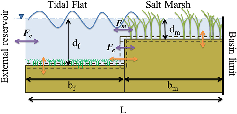
Figure 1. Schematic of the basin. Three independent variables are used to describe the basin geometry: salt marsh depth, d_m, tidal flat depth, d_f, and tidal flat width, b_f. Assuming a fixed width of the basin, L, the marsh width, b_m, is a dependent variable. Changes in configuration (orange) arise from exchange of sediment (purple) from the external reservoir and the tidal flat, F_c, fluxes arising from boundary erosion or accretion, F_e, and the sediment flux to vertical marsh surface from the tidal flat, F_m.

In this model the tidal flat is connected to some external body of water (bay/tidal channel/tidal inlet) which acts as a source of allochthonous sediment. Ignoring SLR, autochthonous sediment production and allochthonous sediment influx, the model conserves the total amount of sediment between two conceptual boxes of unit width defined by three independent variables. These boxes are defined completely by the average marsh platform depth (i.e., water depth above the marsh platform), d_m, average depth to the tidal flat, d_f, both relative to Mean High Water (MHW), and the length of the tidal flat, b_f, provided that the total basin is constrained to a total length L (Figure 1). In this manner, any change in the tidal flat depth or tidal flat length due to wind wave erosion affects both the depth and width of the marsh platform, and vice versa.

Changes in tidal flat length with time, $\stackrel{•}{b_f}$ are constrained by the difference between marsh boundary erosion, B_e [LT⁻¹], and marsh boundary progradation, B_a [LT⁻¹].

$\begin{array}{ll}\stackrel{•}{b_f}=\left[B_e-B_a\right]& (1)\end{array}$

Following Mariotti and Fagherazzi (2010), the erosion of the marsh boundary, B_e, is linearly proportional to the wave power density (W m⁻¹) at the marsh boundary with an erodibility coefficient k_e set to 0.16 m year⁻¹ (Mariotti and Carr, 2014). Marsh progradation, B_a, is set proportional to the suspended sediment concentration (SSC) on the tidal flat, with an empirical coefficient of proportionality k_a = 2 (Mariotti and Carr, 2014).

Wave characteristics are calculated following Mariotti and Fagherazzi (2013) using the formulation of Young and Verhagen (1996) based on wind speeds 10 m aloft. The wave generated shear stress acting on the sediment surface is estimated by ${\tau }_{wave}=\frac{1}{2}{f}_w\rho {\left(\frac{\pi H_s}{T_{p}sinh(kh)}\right)}^2$ given water depth, h, significant wave height, H_s, wave number, k, wave period, T_p, ρ is water density, and the wave friction factor parameter, f_w, which is calculated following Lawson et al. (2007). The wave power density acting on the salt marsh scarp is also estimated from these wave parameters (Schwimmer, 2001; Mariotti and Fagherazzi, 2010).

Changes in marsh platform elevation with time are computed as:

$\begin{array}{ll}\stackrel{•}{d_m}=-\left[F_m+O\right]/\rho +R,& (2)\end{array}$

where F_m [ML⁻²T⁻¹] is the sediment flux exchanged with the tidal flat, O [ML⁻²T⁻¹] is the organogenic sediment production, computed as function of the standing biomass, and R [LT⁻¹] is the rate of sea level rise (Mariotti and Carr, 2014). The flux between tidal flat and salt marsh is computed through the tidal dispersion mechanism, F_m = [C_r − C_m] min [r, d_m]/T_ω, where r is the tidal range, T_ω is the tidal period, C_r is the reference SSC on the tidal flat and C_m is the reference SSC on marsh platform. The reference concentration on the tidal flat is estimated as proportional to the excess shear stress $S=\frac{{\tau }_{wave}-{\tau }_{cr}}{{\tau }_{cr}}$ following Smith and McLean (1977) with $C_r={\rho }_s\frac{\lambda S}{1+\lambda S}$ where ρ_s is the sediment density and λ is an erosion parameter which is here set to 0.0001. The reference concentration on the salt marsh is computed analogously to that on the tidal flat, using the salt marsh depth to compute the τ_wave. In addition, when marsh vegetation is present, this concentration is set equal to zero (Marani et al., 2010), accounting for the significant wind wave dissipation promoted by the vegetation.

The change in tidal flat depth with time is controlled by three terms,

$\begin{array}{ll}\stackrel{•}{d_f}=\left[B_e-B_a\right]\left[d_m-d_f\right]/b_f+\left[(b_m/b_f)F_m+F_c\right]/\rho +R.& (3)\end{array}$

The first term is the redistribution of sediment eroded/accumulated at the marsh boundary. The second term is the net flux of sediment from the flat to the marsh, and represents the dispersive fluxes exchanged with the salt marsh and the some external adjacent body of water, F_c = [C_r − C_o] min [r, d_f]/T_ω, where C_o is the external suspended sediment concentration. It can be noted that B_a, B_e and F_m redistribute the sediments within the marsh-flat system, while the terms F_c and O allow for net sediment loss or gain.

This simple model allows us to investigate coupled salt marsh-tidal flat dynamics without seagrass. A more detailed model description and behavior can be found in Mariotti and Carr (2014). Because the model assumes that allochthonous sediment must first pass onto the tidal flat before being resuspended and delivered to the marsh platform, the tidal flat acts as a geomorphologically active system that is directly coupled to the salt marsh. Application of the model to conditions at the VCR allows for examination of the impact of seagrass on this coupled system.

The Bio-Morphodynamic Submodel for Seagrass on the Tidal Flat

Seagrasses can play an important role in modifying the wave environment, especially when they fill a large fraction of the water column (Fonseca and Cahalan, 1992; Méndez et al., 1999; Chen et al., 2007; Bradley, 2009; Hansen and Reidenbach, 2012). While seagrasses can modify significant wave height and wave period, near bed orbital velocities and shear stress are less affected (Heide et al., 2007; Hansen and Reidenbach, 2012). To this end, the effect of submerged vegetation on the wave-induced shear stress was modeled by the attenuation of significant wave height through the wave attenuation coefficient:

$\begin{array}{ll}{a}_{Hs}=1-\left(\frac{N}{N_{Hs}+N}\right)& (4)\end{array}$

where N is shoot density, and N_Hs is the half saturation constant for attenuation set here at 400 shoots m⁻² following measurements from Hansen and Reidenbach (2012, 2013), and Thomas (2014). Wave height attenuation only occurs if the wave period is large enough interact with the canopy, e.g., $1/T_p<\sqrt{4\pi g(h-h_{can})}$ where h_can, is the canopy height and g is gravitational acceleration.

Provided the wind speed at 10 m aloft, U₁₀, nondimensional wave energy, ε, calculated following Young and Verhagen (1996), and the wave attenuation coefficient a_Hs (Equation 4), significant wave height can be calculated as:

$\begin{array}{ll}{H}_s=4a_{Hs}\sqrt{\frac{\epsilon U_{10}^4}{g^2}}& (5)\end{array}$

In general, wave attenuation by vegetation is complex and can depend on the relative velocity of the canopy to the wave orbital velocity, leaf and shoot morphology, and canopy bending among others factors (Méndez et al., 1999). However, the addition of this complexity is beyond the scope of this simple model.

In order to account for temporal changes in shoot density within the tidal flat a simple logistic growth model similar to the model of Heide et al. (2007) was utilized to estimate rate-of-change in shoot density:

$\begin{array}{ll}\frac{dN}{dt}=n_{grow}g(I,T)N\left[1-\frac{N}{N_{cc}}\right]-f(T)n_{mort}N& (6)\end{array}$

where the maximum specific growth rate n_grow = 0.08 day⁻¹ (Heide et al., 2007) is modified by both the light environment, I, and temperature g(I,T), with a maximum shoot density, N_cc = 1000 shoots m⁻². Mortality is a constant fraction of shoot density n_mort = 0.013 day⁻¹, modified by water temperature, $f(T)={{\theta }_T}^{(T-20)}$, with θ_T set to 1.05 following Zharova et al. (2001) and Carr et al. (2012). While other characteristics besides light, depth and temperature contribute to determining seagrass growth and consequent depth limitations (Koch, 2001), a sediment modified light environment was used here to focus on the feedbacks between seagrasses, sediment resuspension, and the wave environment. The flat depth is modeled as a single elevation and seagrasses are assumed to fully cover the tidal flat if light conditions are favorable for their establishment and growth. To this end a light limitation function is defined as

$\begin{array}{ll}g(I,T)=\left\{\begin{array}{cc}\frac{I-I_C(T)}{I_K(T)-I_C(T)}& I_C<I<I_K\\ 1& I\ge I_K\\ 0& I\le I_C\\ \end{array}\right\}& (7)\end{array}$

where I is the photosynthetically active radiation (PAR) reaching the sediment surface, I_K is the saturation irradiance value calculated as:

$\begin{array}{ll}{I}_K=I_{K20}{\theta }_K^{T-20}& (8)\end{array}$

and I_C is the compensation irradiance, calculated as:

$\begin{array}{ll}{I}_C=I_{C20}{\theta }_C^{T-20}& (9)\end{array}$

with I_K20 and I_C20 being the saturation and compensation irradiance at 20°C respectively.

The PAR reaching the sediment surface is determined following the Lambert-Beer Equation:

$\begin{array}{ll}I=I_0{e}^{-K_d{d}_f}& (10)\end{array}$

given seasonally varying PAR, I₀, and water temperature, T (Figure SI1, Porter et al., 2014). The water column light attenuation coefficient K_d is site specific, and affected by multiple water column characteristics including, but not limited to, total suspended solids, colored dissolved organic matter, and chl a (Gallegos, 2001). Here the attenuation coefficient is based on the equation from Lawson et al. (2007), developed for a central bay in the VCR, which depends primarily on suspended sediment concentration. SSC used for light attenuation, C_t, is calculated as an average of the external allochthonous supply, C_o and the resuspended sediment concentration on the tidal flat, C_r.

$\begin{array}{ll}{C}_t=\frac{C_r{d}_f+C_{o}r}{2(d_f+r)}+\frac{C_r}{2}& (11)\end{array}$

In this manner as external sediment loading increases, the light condition on the tidal flat deteriorates described by Equation 7. Interaction of parameter choices for seagrass (Table 1) and the seasonal drivers (Figure SI1) results in shoot densities of 0–700 shoots m⁻², similar to those found in the VCR (McGlathery et al., 2012).

TABLE 1

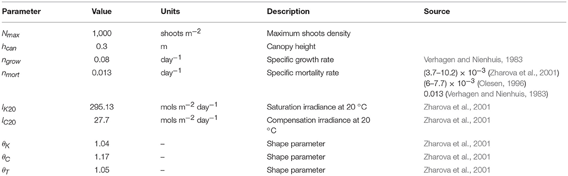
Table 1. Seagrass model parameters and sources.

Hourly wind speed measured at National Data Buoy Center station CHVL2 were acquired for 1984 to 2015 (NOAA, 2017a,b) and all winds were rescaled to 10 m aloft assuming a fully rough sea surface (SethuRaman and Raynor, 1975). To account for autocorrelation and seasonality in the hourly wind speed record, a 4th order Markov Chain Monte Carlo approach (Karatepe and Corscadden, 2013) was used to generate synthetic hourly time series of wind speed and direction. Monthly transition probability matrices, where the probability of a given wind speed and direction for any hour of the year is based on wind speed and direction during the prior 2 h, were calculated in order to capture the strong seasonality in wind speed at the VCR, characterized by both high winds speeds and increased variability in the winter months (Table SI1). Similar seasonality is achieved in the synthetic record (Tables SI1, SI2).

Model Behavior Under Constant Drivers

Stability and trajectories of the coupled marsh-flat system were explored by examining the nullcline surfaces (e.g., the surfaces in d_f, d_m, b_f space where $\stackrel{•}{d_f}=0$, $\stackrel{•}{d_m}=0$, and $\stackrel{•}{b_f}=0$). Intersections of these equilibrium surfaces, or lack thereof, are difficult to visualize (Figure SI2), so we rely on the differences in rates of adjustment of flat depth, marsh depth and tidal flat width to their respective equilibrium surface to reduce dimensionality. Tidal flat depth and width adjusts faster (~m-cm year⁻¹) than the depth the marsh platform (~mm year⁻¹). However, these rates relative to their respective nullclines (i.e., $\frac{\stackrel{•}{d_f}}{d_{f,equil}}>\frac{\stackrel{•}{d_m}}{d_{m,equil}}$ $>\frac{\stackrel{•}{b_f}}{b_{f,equil}}$) with, d_{f, equil} (~m), d_{m, equil} (~cm), b_{f, equil} (~km) indicate that the tidal flat depth adjusts to the nullcline depth, followed by adjustment of the marsh platform depth and slower adjustment of the tidal flat width.

As an example, model run trajectories (Figure 2A, black) for RSLR = 4 mm year⁻¹, Co = 30 mg/L and constant wind speed, $U_{const}=\overline{U}=$ 6.87 m s⁻¹, shows movement toward and then along the nullcline depth surface (Figure 2A, blue). This tidal flat depth equilibrium surface (blue lines Figure 2A) can be represented by contours in the plane of tidal flat width and marsh depth (Figure 2B). Assuming the system is at the equilibrium tidal flat depth (Figure 2B), changes in tidal flat width, $\stackrel{•}{b_f}$(Figure 2C, red), and marsh depth, $\stackrel{•}{d_m}$(Figure 2D, green), along the tidal flat depth nullcline surface, depth_nc, can be examined for a constant set of parameters (e.g., constant wind speed, U_const, seagrass density, N_const). In this manner it is apparent if a system at equilibrium depth is eroding or prograding (positive or negative red contours respectively), and if the marsh is experiencing vertical accretion or loss (positive or negative green contours respectively). This allows for simplification in visualizing both behaviors and potential unstable and stable equilibria of the system (where contours of $\stackrel{•}{d_m}=0$and $\stackrel{•}{b_f}=0$ intersect).

FIGURE 2

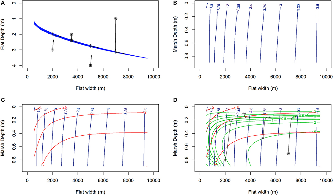
Figure 2. (A) The collection of tidal flat depth nullclines (blue lines) and 1000 year trajectories (black) of the system showing little lateral change until the nullcline depth has been reached for RSLR = 4 mm year⁻¹, Co = 30 mg/L and constant wind speed, $U_{const}=\overline{U}=$ 6.87 m s⁻¹. (B) Those same nullclines, or nullcline plane, now shown as contours of tidal flat depth (m) in the plane of tidal flat width and marsh depth. (C) Contours are added showing curves of constant rate of change (m/year) of tidal flat width (red) along the surface defined by the tidal flat depth nullcline contours (blue). In this case, for almost all flat width and marsh depths, the system would exhibit lateral erosion. Positive and negative values signify lateral erosion and progradation respectively, the thick red line represent where the lateral erosion rate is zero. (D) Addition of the contours of marsh depth rates of change (mm/year, green) along the same tidal flat depth nullcline surface and trajectories of the system initiated on the nullcline surface. Positive and negative values signify vertical accretion and loss respectively, the thick green line represent where the marsh vertical accretion rate is zero. Again as the system is initiated along the tidal flat depth nullcline surface (B), trajectories (D, black) exhibits lateral erosion and progression to a equilibrium marsh depth.

For these constant driver runs, the constant wind speed was determined from a 500 year long synthetic time series and set equal to either the temporal average wind speed, $U_{const}=\overline{U}$, or the 85th percentile of wind speed, U_const = U₈₅, and behaviors of tidal flat width and marsh depth adjustments rates were examined along the $dept{h}_{nc\overline{U}}$ and depth_ncU85 surfaces both with and without seagrass.

Under most conditions, clear erosional or progradational behavior of the bay-marsh boundary, and thus the system, is apparent. As external sediment loading increases (10, 30 to 50 mg L⁻¹) a the lateral erosion rates diminish, and there is a shift from an erosional to progradation system for narrow flat widths (Figures 3A,B, 4A,B, 5A,B). Similarly, the depth the marsh platform decreases as external sediment loading increases (Figures 3A,B, 4A,B, 5A,B). Depending on model parameters, unstable equilibria appear under some scenarios (Figures 5A,B).

FIGURE 3

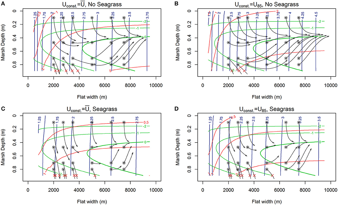
Figure 3. Contours of lateral rates of change in tidal flat width (m /year, red), and vertical changes in marsh depth (mm/year, green) alongside 1000-year trajectories (black) of the system initiated at various tidal flat widths and marsh depths along the tidal flat depth nullcline surface (blue contours) for various winds (RSLR = 4 mm year⁻¹, Co = 10 mg/L). (A) Constant wind ($U_{const}=\overline{U}=$ 6.87 m s⁻¹), no seagrass, red contours indicating erosions, and marsh drowning of low-lying marshes with fetches up to 4 km exhibited by trajectories ending with red x. (B) Constant but higher wind (U_const = U₈₅ = 8.5 m s⁻¹), no seagrass, showing faster erosion, deeper flat, and only very low-lying marshes drowning for fetches <3.5 km. (C) Constant wind and seagrass ($U_{const}=\overline{U}=$ 6.87 m s⁻¹, N = 250 shoots m⁻²) showing reduced erosion of the salt marsh and a shallower system with ‘enhanced’ drowning of low-lying marshes up to fetches of 5 km. (D) Constant higher wind with seagrass (U_const = U₈₅ = 8.5 m s⁻¹, N = 250 shoots m⁻) showing erosion and drowning of low-lying marshes up to fetches of 5 km.

FIGURE 4

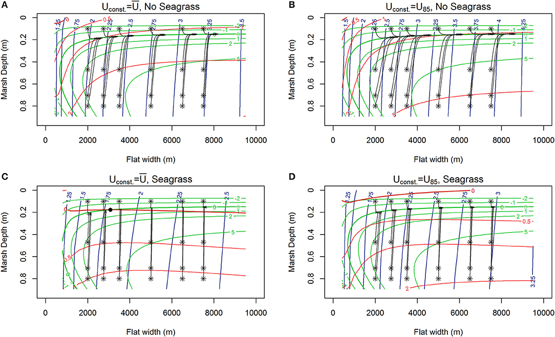
Figure 4. Contours of lateral rates of change in tidal flat width (red), and vertical changes in marsh depth (green) from MHW alongside 1,000 year trajectories (black) of the system initiated at various tidal flat widths and marsh depths along the tidal flat depth nullcline surface (blue contours) for various wind conditions, RSLR = 4 mm year⁻¹, Co = 30 mg/L. (A) Erosion, no seagrass, marshes maintaining pace with RSLR ($U_{const}=\overline{U}=$ 6.87 m s⁻¹). (B) Faster erosion, no seagrass, marshes maintaining pace with RSLR (U₈₅ = 8.5 m s⁻¹). (C) Appearance of stable equilibria (C, black dot) in the presence of seagrass at around 3 km wide tidal flat, marshes maintaining pace with RSLR ($U_{const}=\overline{U}=$ 6.87 m s⁻¹, N = 250 shoots m⁻²). (D) Slow erosion in the presence of seagrass, with marshes maintaining pace with RSLR (U₈₅ = 8.5 m s⁻¹, N = 250 shoots m⁻²).

FIGURE 5

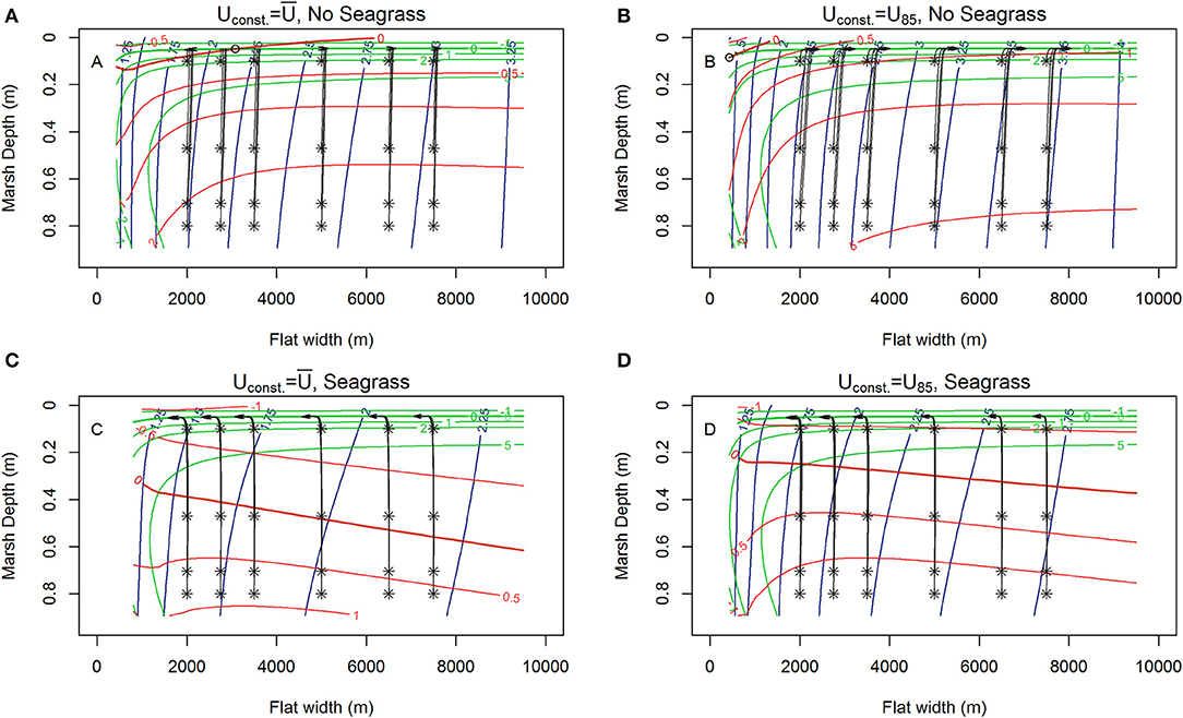
Figure 5. Contours of lateral rates of change in tidal flat width (red), and vertical changes in marsh depth (green) from MHW alongside 1,000 year trajectories (black) of the system initiated at various tidal flat widths and marsh depths along the tidal flat depth nullcline surface (blue contours) for various wind conditions, RSLR = 4 mm year⁻¹, Co = 50 mg/L. (A) Unstable equilibria (open circle) with erosion or progradation depending on flat width., no seagrass, marshes maintaining pace with RSLR ($U_{const}=\overline{U}=$ 6.87 m s⁻¹). (B) Shift of unstable equilibria (hollow circle) to vary narrow flat widths, no seagrass, marshes maintaining pace with RSLR (U₈₅ = 8.5 m s⁻¹). (C) Shift to prograding system in the presence of seagrass, marshes maintaining pace with RSLR ($U_{const}=\overline{U}=$ 6.87 m s⁻¹, N = 250 shoots m⁻²). (D) Shift to progradation in the presence of seagrass, but slower progradation rate due to higher winds, with marshes maintaining pace with RSLR (U₈₅ = 8.5 m s⁻¹, N = 250 shoots m⁻²).

If a constant density of seagrass (N_const = 250 shoots m⁻²) is added, we see some erosional configurations without seagrass shift to progradational in the presence of seagrass, with all cases exhibiting significantly shallower tidal flat depth, and a slightly increased marsh depth (Figures 3–5). Interestingly, at small tidal flat widths (concurrent wide marsh platform), low-lying salt marsh and small external sediment loading, the presence of seagrass inhibits the ability of the marsh platform to maintain pace with SLR (Figures 3C,D, RSLR = 4 mm year⁻¹, C_o = 10 mg L⁻¹). Conversely, in a system with higher external sediment loading the marsh platform keeps pace with sea level rise and the introduction of seagrass also produces stable equilibria under specific constant wind conditions (Figure 4C, RSLR = 4 mm year⁻¹, Co = 30 mg L⁻¹). However, a change in the constant driving wind conditions U_const = U₈₅ from average wind speed $\overline{U}$ to U₈₅ removes the stable equilibria (Figure 4D), indicating that persistent presence of a stable equilibria under stochastic drivers (e.g., variable wind speed) is unlikely.

Different drivers (U_const, RSLR, C_o) and presence/absence of seagrass generates three general behaviors: erosional (Figure 3), progradational (Figure 5), and drowning (trajectories ending in red x in Figure 3, Figure SI3). On top of these three general behaviors, the system under constant drivers is either (1) unstable, (Figure 5A) or (2) stable, prograding or eroding to some stable configuration (Figure 3C) depending on the initial state (d_f, d_m, b_f) of the system.

Model Behaviors Under Variable Drivers

Long-term model behavior over 500 years was explored for external sediment supplies of 10–40 mg/L and RSLR scenarios of 3–6 mm/year for flat widths of 500–7,000 m initiated at the associated bare sediment equilibrium depth along nc_U85 as defined in the constant wind speed runs (Figure 6). Shorter-term behavior (300 year model runs) was explored for tidal flat depths of 1.5–5 m and tidal flat widths of 0.5–7.5 km (RSLR = 4 mm year⁻¹, C_o = 30 mg L⁻¹) in 0.25 m and 0.25 km increments respectively (Figure 7). All scenarios were run using synthetic stochastic seasonal winds averaged over a tidal cycle, and stochastic water temperatures with a time step of a tidal cycle (12.5 h). Each modeled scenario used a constant rate of RSLR and external sediment supply, and a constant seasonal cycle of PAR (Figure SI1) for a basin width, L = 10 km. Seagrass was initiated at 1 shoot m⁻² and allowed to either die off or increase depending on light conditions. These model runs were then compared to identical runs with no seagrass and with seagrass initiated at 500 shoots m⁻².

FIGURE 6

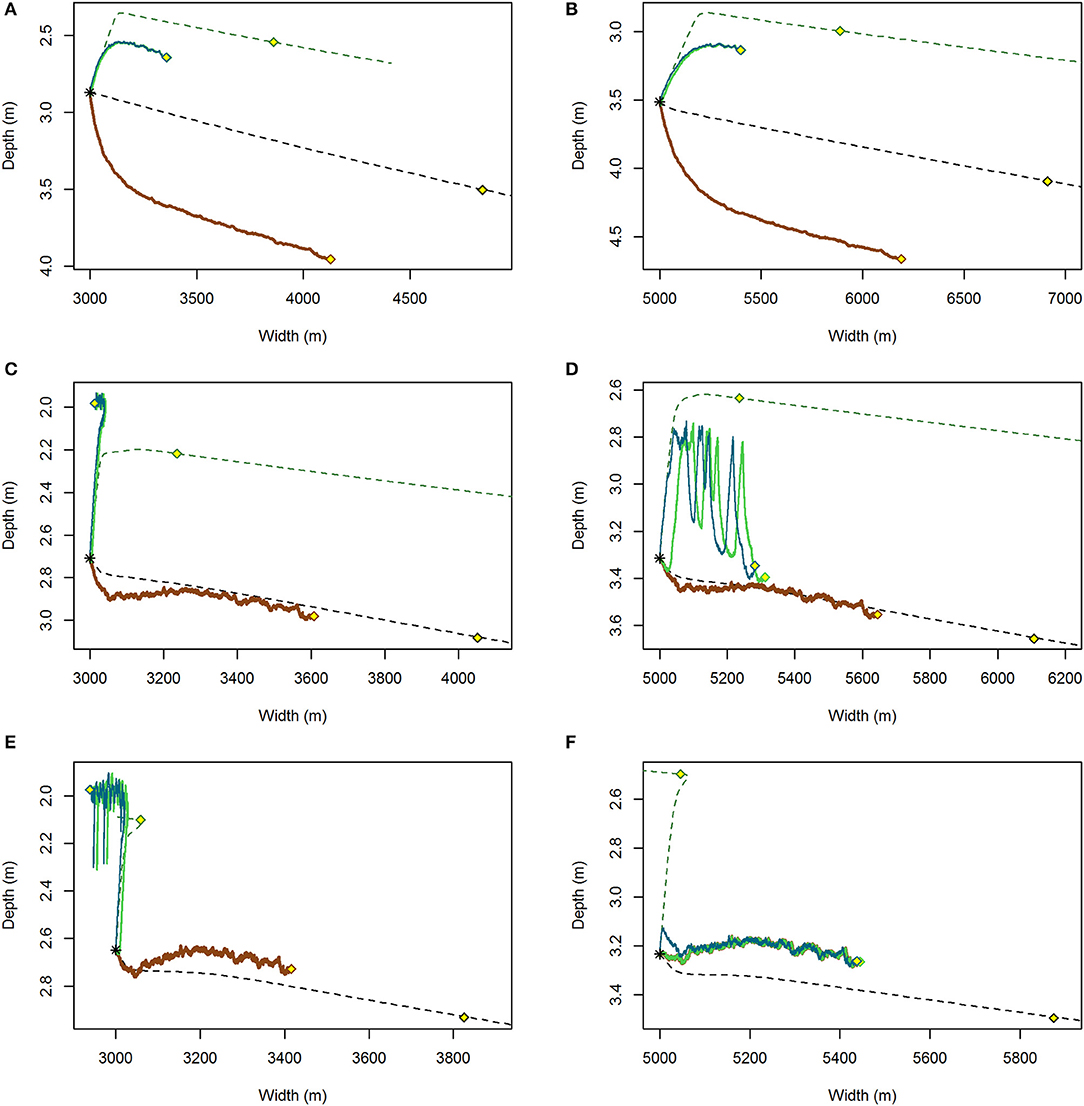
Figure 6. Variable (solid) and constant wind (dashed) trajectories of tidal flat depth and width for the coupled system initiated at a tidal flat width of 3,000 m (A,C,E) and 5,000 m (B,D,F) for RSLR = 4 mm year⁻¹ and (A,B) Co = 10 mg/L, (C,D) Co = 30 mg/L, (E,F) Co = 40 mg/L. The smooth dashed lines represent trajectories under a constant wind U₈₅ = 8.5 m s⁻¹ for a system without seagrass (black line) and with seagrass (green line). Superimposed are trajectories under variable wind without seagrass (brown), with the possibility of seagrass to establish from 1 shoot m⁻² (green), and 500 shoots m⁻² (blue). Points (yellow) along each line represent the state of the system after 500 years.

FIGURE 7

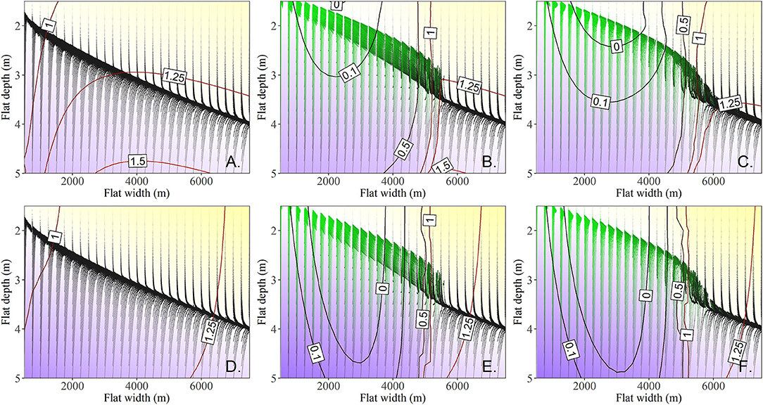
Figure 7. 300 year long trajectories initiated at tidal flat depths of 1.5–5 m and tidal flat widths of 0.5–7.5 km (RSLR = 4 mm year⁻¹, C_o = 30 mg L⁻¹) in 0.25 m and 0.25 km increments respectively. Yellow regions indicate where trajectories result in overall deepening of the tidal flat whereas blue regions represent shallowing system trajectories. The white region represents the vertical nullcline. Contours of the lateral erosion rate (total lateral erosion rate (A–C), final five year average erosion rate (D–F) are shown. (A) and (D), are systems with no seagrass allowed. (B,E), Seagrass is allowed to establish, or senesce. (C,F), Seagrass is initiated at 500 shoots m⁻² and allowed to establish, or senesce.

Model behavior and results under stochastic winds were different than those obtained with constant winds. For model runs with C₀ < 30 mg L⁻¹, the tidal flat depth-width trajectories were consistently deeper than nc_U85 (Figures 6A,B). At 30 mg L⁻¹ and RSLR of 4 mm year⁻¹ the trajectories followed closely nc_U85 for tidal flat widths >5,000 m (50% of the total basin width, Figures 6C,D) similar to the effective wind speed estimated by Mariotti and Carr, 2014. At C₀ >40 mg L⁻¹, the system under stochastic drivers was consistently shallower (Figures 6E,F).

The establishment of seagrass on the tidal flat resulted in a shallower tidal flat system across all sediment loading and sea-level rise scenarios (Table 2). In contrast to the stable equilibria (Figure 4C) or erosion (Figure 4D) predicted under constant drivers when seagrass was present, both a stable equilibrium (Figure 6C) around 2.0 m water depth, and a unstable equilibrium, as noted by the erosive behavior larger tidal flat width (Figure 6D) emerge. Seagrass extant at smaller fetches (narrower flats) than the unstable equilibria remain in the attractive domain of a stable equilibria, while those at larger fetches possess a limited lifespan as the salt marsh slowly and continually erodes, the tidal flat deepens, and light conditions deteriorate (Figures 6D, 8). For all runs, erosion rates under stochastic forcing were less than those under constant forcing (yellow points Figure 6).

TABLE 2

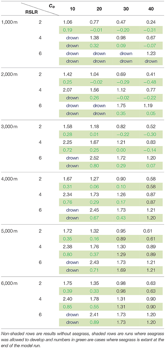
Table 2. Comparison between average lateral erosion/progradation rates (± m year⁻¹) of the salt marsh for 500 year model runs initiated at flat widths of 1–6 km, sea level rise rates of 2–6 mm year⁻¹ and external sediment loading of 10–40 mg/L.

FIGURE 8

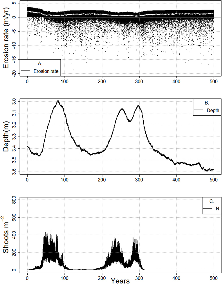
Figure 8. Cyclical meadow behavior and concurrent changes in tidal flat erosion rate (A), tidal flat depth (B), and shoot density (C) during the 500-year-long model runs (RSLR 4 mm year⁻¹, Co = 30 mg/L, b_f = 5.25 km). Decadal to half century long cycles of this behavior are noted.

To examine the depth limit for seagrass, and the locations of the unstable and stable equilbiria, we ran the model for 300 years with the same sequence of stochastic drivers in 250 m width increments along nc_U85 for 30 mg/L and RSLR of 4 mm/year with meadows initiated at 1 (Figures 7B,E) and 500 shoots m–² (Figures 7C,F). By 5.4 km and 3.3 m water depth seagrass was unable to fully establish. However, meadows initiated at 500 shoots m–² were able to persist for up to ~30 years before collapsing, and a fold bifurcation emerged from ~3.3 to 3.6 m depth and bay widths of ~5.4–6.1 km for that specific sequence of stochastic winds. A different sequence of stochastic winds under the same constant drivers of RSLR and sediment loading from the 500-year model runs showed meadow collapse from 4.5 to 5 km bay widths at ~3.2 m depth, and the inability of a meadow to establish at bay widths >5 km and depths >3.25 m.

Examining the total erosion rate (contours in Figures 7A–C) shows the impact of the system starting away from a stochastic nullcline depth surface, as well as the broad impact of seagrass on tidal flat depth. Once the system has adjusted vertically, the average erosion rate over the last 5 years of the model run (contours Figures 7D–F) clearly indicates the presence and general location of stable and unstable equilibria in the presence of seagrass (zero erosion contour line Figures 7E,F). It is interesting to note that the unstable equilibria for meadows establishing from 1 shoots m⁻² occurs around 2.2 m water depth and a flat width of 3.75 km (Figure 7E), whereas for meadows established at 500 shoots m⁻² this unstable equilibria occurs at around 4 km tidal flat width and 2.3 m water depth. This indicates that while there is a depth bifurcation with regards to seagrass establishment, there is also a lateral bifurcation (~250 m) which indicates if a meadow will persist over a longer time scale (i.e., if it is one side of the unstable equilibria or the other).

Cyclical Behaviors Induced by Light-Dependence

Interestingly, as the tidal flat widens and deepens, cyclical behavior in shoot density and tidal flat depth was present (Figures 6D, Figure SI4), in which the system behaves coherently for decades in a bare sediment state before switching to a vegetated state. Decadal long cycles of this behavior are noted prior to full collapse of the meadow (Figures 6D, 7, 8, Figure SI4). The vegetated state maintains an overall better light environment across a range of depths until some shallow depth is reached (Figure 8B), at which point an increase in wave resuspension of sediment deteriorates the light environment. This poorer light environment is maintained during the continual deepening and collapse to an unvegetated deeper tidal flat. Eventually, the wave stress diminishes due to increased water depth, resulting in an improvement in light conditions and potential subsequent reestablishment of seagrass (Figure 8C). As a result, slow recovery to a shallower system occurs until another eventual collapse (Figure 8B).

This cyclic behavior does not last indefinitely. The tidal flat is continually widening (Figure 8A) and deepening (Figure 8B) through time due to wind wave erosion of the salt marsh scarp, with consequent decline in the benthic light environment. Eventually the light conditions are so poor that the system only exhibits an unvegetated state (Figure 8C). In other words, alongside a depth limit for establishment, as fetch increases, a fetch-dependent shallow depth limit emerges above which seagrass cannot persist. Once the flat is wide enough for this to occur, the system begins to cycle in depth and shoot density, then fully oscillates between a bare and vegetated states. Finally the fetch-dependent shallow depth limit coincides with the bare state depth nullcline and no further oscillations occur.

These decadal time-scale cycles may have important implications for our understanding of the stability of either a bare or seagrass-dominated system state, especially as they may also exist in the attractive domain of some stable equilibrium (Figure 9). This complex behavior in establishment and maintenance of seagrass suggests that the depth, width, and the presence and significance of alternate state dynamics depends critically on the interaction of the state of the system and on the sequence of external drivers.

FIGURE 9

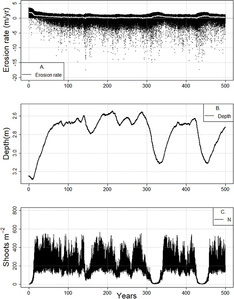
Figure 9. Cyclical meadow behavior and concurrent changes in tidal flat erosion rate (A), tidal flat depth (B), and shoot density (C) during the 500-year-long model runs (RSLR 4 mm year⁻¹, Co = 30 mg/L, b_f = 3.0 km) for a prograding marsh system.

Discussion

For the shallow coastal bays of the VCR, the presence or absence of seagrass altered the picture depicted in the simple model of Mariotti and Carr (2014), which demonstrated the dual role of wind waves on salt marsh stability. While lateral erosion of the salt marsh overall promotes vertical stability of the salt marsh platform, the presence of seagrass provides a strong lateral stabilizing effect on the coupled system, with lateral migration rates reduced from m-cm to cm-mm per year, and shallower tidal flats in comparison to a system without seagrass. In some cases the system switched from a retreating to a prograding marsh, even under low allochthonous sediment supply (Table 2). In scenarios considering high rates of sea level rise, low sediment loading and/or small tidal flats, the seagrass tended to act as a sediment sink, overall decreasing the sediment supply to the salt marsh and consequently increasing the susceptibility of the salt marsh to drowning. Moreover, with reduced lateral erosion rates, the increases in wave regime and sediment supply associated with the retreat of the marsh boundary occur more slowly, also increasing the potential for the salt marsh to drown. In this regard, seagrass maintains shallow tidal flats with better light conditions at the expense of the adjacent marsh platform (Table 2). In contrast, if the tidal flat is wide enough, seagrasses act in a beneficial way to the marsh by both maintaining shallower tidal flat depths and reducing wave energy acting on the marsh boundary. It seems logical that a shallower, vegetated flat should come at the expense of the salt marsh depth because of lower suspended sediment concentrations, and therefore reduced sediment flux to the salt marsh platform. However, due to senescence of vegetation in the fall and winter combined with shallow water depths, increased flux to the salt marsh is also possible. Rescaling the flux to the marsh by the ratio of tidal flat depth to tidal flat width (e.g., F_md_f/b_f), normalized fluxes to the salt marsh system from the tidal flat with and without seagrass are similar in magnitude with strong seasonal differences, despite different fetch and depth conditions (Figure 10). Thus, if the tidal flat is wide enough, the presence of seagrass can provide a stabilizing effect on the marsh boundary, while still supplying enough sediment to the salt marsh for it to maintain pace with sea-level rise.

FIGURE 10

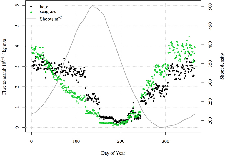
Figure 10. Daily bin-averaged shoot density and daily bin-averaged scaled sediment flux (F_md_f/b_f) to the salt marsh with (green) and without seagrass (black) from 500 year-long model runs initiated with RSLR = 4 mm year⁻¹, Co = 30 mg L⁻¹ and an initial tidal flat width of 4 km. Note the decrease in flux during spring and early summer alongside increases in shoot density, and enhanced flux during the fall due to the seasonal seagrass senescence.

Interestingly, long term oscillations in the state of the system display a reduction in erosion or increase in progradation when a meadow is lost due to increased wave resuspension of sediment from the tidal flat (Figures 7A, 8A). Similarly, when a meadow re-establishes, there is an increase in lateral erosion because the presence of seagrass reduces resuspension. This reduction or enhancement in erosion is transitory while the system moves from a vegetated to unvegetated state or the reverse.

In cases where the salt marsh continues to erode, increased fetch (accompanied by deeper flats, larger waves and poorer light conditions) will eventually result in conditions that cannot support the presence of seagrass. However, prior to the system being fully unable to support seagrass, the state of the system may oscillate between shallow and deeper flats and the presence and absence of meadows. This behavior might be thought of as a type of flickering (Scheffer et al., 2001, 2012; Carpenter and Brock, 2006; Scheffer, 2009) that exhibits a slow oscillation rather than a rapid transition between states. Similarly, the reduction in shoot density in subsequent oscillations could be thought of as a damped oscillator, or a critical slowing down of the system (van Nes and Scheffer, 2007; Dakos et al., 2008; Biggs and Carpenter, 2009; Scheffer et al., 2012). In the case of an eroding system, this oscillatory behavior is indeed indicative of long term collapse to a bare state (Figures 8, Figure SI4). However, if a system is prograding (Figure 9), such oscillations do not necessitate loss of a vegetated state.

These results pose a conundrum when interpreting the results of observational studies of systems exhibiting bistable behavior, such as bimodality in a distribution: is the bimodality an indicator of true alternative stable states or might it be associated with longer term oscillatory behavior? Is it possible for system to maintain a limit cycle? In our results the oscillations are transitory and not a limit cycle, but care should likely be taken when attributing alternate state dynamics, especially as behavior at longer time scales is uncertain.

The concept of marsh stability is difficult to define in that horizontal and vertical equilibrium is tenuous at best (Fagherazzi, 2013). However, our results show that horizontal and vertical coupling allows for a more stabilized system due to feedbacks between fetch, wind waves and erosions and sediment fluxes. The presence or absence of seasonally varying seagrass has the potential to both increase and decrease the resilience of the system as a function of the basin geometry. For large salt marshes coupled to small flats, the presence of seagrass exacerbates the potential for drowning. For larger tidal flats, seagrass stabilizes both tidal flat depth and width (e.g., reduces erosion rates), and at the same time allows for seasonal sediment fluxes to the salt marsh (Table 2, Figure 10).

While long-term changes in the configuration of the marsh-flat system occur on time scales longer than the variability in wind wave and light conditions, model results using representative constant forcing rather than variable wind speed and water temperature produced discrepant behavior. For example, constant representative winds applied a constant shear stress to the tidal flat and a constant wave power to the scarp edge resulting in much higher lateral marsh erosion rates compared to model results using stochastic forcing. Similarly, seasonally varying vegetation altered the behavior of the coupled system. This indicates that seasonality of the drivers and vegetation are both important when considering the co-evolution of the system.

Some generalities however can be drawn from our results. First, the presence of seagrass overall acts to reduce marsh erosion rates (Table 2, Figure 7). Second, for large marshes coupled to small bays the presence of seagrass may exacerbate drowning as seagrasses act to sequester sediment. As SLR rates increase, this is more likely to occur. Third, presence of seagrass has more impact on erosion rates than increased sediment loading to the system (Table 2).

As with any model, simplifications and/or omissions can result in poor representations of real processes. While this model considers key feedback mechanisms affecting system behavior, care should be taken when interpreting results. For example, the depth of the Bay is idealized by a single representative depth, ignoring irregular bathymetry which would affect both wave growth and dissipation as well as currents and sediment redistribution. Sediment is represented by a single settling velocity, rather than a grain size distribution, which varies spatially in the Bay system (Wiberg et al., 2015). The salt marsh in this model is assumed to capture all of the sediment that is delivered to it. Moreover, because there is no explicit salt marsh vegetation, seasonality in above ground salt marsh biomass and capture efficiency is ignored. Similarly, the impact of seagrass root and rhizome mat on sediment resuspension is not well understood and not included. Impacts of the presence of seagrass on tidal currents, which are only implicitly accounted for by tidal dispersion, was also ignored as the VCR is dominated by wind wave resuspension (Lawson et al., 2007). These simplifications likely impact mineral sediment accretion rates. All sediment, mineral or organic, is conserved in the model. In reality, refractory carbon material from the salt marsh is likely not conserved and fully deposited onto the tidal flat due to remineralization. Sea-level rise rates and external sediment loading are assumed constant in our model but may vary in time in natural systems. The approach used to generate stochastic wind speeds only reproduces values within the measured distribution, ignoring potential impacts of climate change on increased storminess. As well, the impacts of storm surge and changes to the tidal cycle due to Spring and Neap tides are not included, but likely impact sediment redistribution. Light and water temperature conditions vary considerably, both spatially and temporally. While water temperatures were stochastically generated, only a single seasonal record of PAR was used. These simplifications were necessary, however, to allow us to examine the interactions of drivers, the state of a system and nonlinear feedbacks, potentially leading to new questions. For example, if seagrass promotes shallower bays, how long does it take for bathymetry to adjust after a wholesale loss of seagrass from the system? Given the extirpation of seagrass from the coastal bays of the VCR in the 1930's, is there evidence of an increased export of sediment from the bays to the salt marsh platforms? Is the present recovery merely part of a longer-term cycle? Do seagrasses provide seasonal cyclical pulses of sediment to the salt marsh platform?

Conclusion

Understanding behaviors of intertidal coastal environments is difficult due to nonlinear responses under various drivers including impacts of sea level rise, increases in storminess, temperature, and anthropogenic disturbances. Process-based modeling of the ecogeomorphic processes that define the dynamics of these ecosystems, allows for exploration of how these systems may change through time and generate new hypotheses and research questions. A three-point dynamic model was used to examine how seagrass adjacent to a salt marsh may impact long term morphological behavior under constant and stochastic forcing for different external sediment supply and rates of sea level rise. The presence of seagrass has two effects: (1) it decreases near bed shear stresses thus reducing the sediment flux to the salt marsh platform; (2) it reduces the wave energy acting on the salt marsh scarp, thus reducing boundary erosion. Model results indicate that the reductions in wave power and near bed shear stresses when seagrass is present provide an overall stabilizing effect on the coupled marsh-tidal flat system; but as external sediment supply increases and light conditions decline, the system reverts to that of a bare tidal flat. System behavior differed between constant and seasonally varying stochastic drivers, indicating that the interaction between seasonality and variability of the drivers and vegetation is important to understanding the co-evolution of the coupled seagrass-marsh system.

Data Availability Statement

The model outputs used for this study are available by request to the corresponding author. Wind speed data utilized in this study if freely available from National Oceanic and Atmospheric Administration's (N.O.A.A.) National Data Buoy Center at http://www.ndbc.noaa.gov/station_page.php?station=chlv2.

Author Contributions

JC and GM created the model. JC, GM, SF, PW, and KM all contributed in writing the article. JC generated all graphics and tables.

Funding

JC acknowledges support from the Ecosystems and Land Resources mission areas of the United States Geological Survey. Partial support was provided by Virginia Coast Reserve LTER project, which was supported by National Science Foundation grants DEB-0621014 and DEB-1237733 and a LTER synthesis Grant.

Conflict of Interest Statement

The authors declare that the research was conducted in the absence of any commercial or financial relationships that could be construed as a potential conflict of interest.

The reviewer SZ and handling editor declared their shared affiliation.

Supplementary material

The Supplementary Material for this article can be found online at: https://www.frontiersin.org/articles/10.3389/fenvs.2018.00092/full#supplementary-material

References

Allen, J. (2000). Morphodynamics of holocene salt marshes: a review sketch from the Atlantic and Southern North Sea coasts of Europe. Quat. Sci. Rev. 19, 1155–1231. doi: 10.1016/S0277-3791(99)00034-7

CrossRef Full Text | Google Scholar

Allen, J. R. L. (1990). Salt-marsh growth and stratification: a numerical model with special reference to the Severn Estuary, southwest Britain. Mar. Geol. 95, 77–96. doi: 10.1016/0025-3227(90)90042-I

CrossRef Full Text | Google Scholar

Biggs, R., and Carpenter, S. (2009). Turning back from the brink: detecting an impending regime shift in time to avert it. Proc. Natl. Acad. Sci. U.S.A. 106, 826–831. doi: 10.1073/pnas.0811729106

PubMed Abstract | CrossRef Full Text | Google Scholar

Bradley, K. (2009). Relative velocity of seagrass blades: implications for wave attenuation in low-energy environments. J. Geophys. Res. 114:F01004. doi: 10.1029/2007JF000951

CrossRef Full Text | Google Scholar

Carpenter, S. R., and Brock, W. A. (2006). Rising variance: a leading indicator of ecological transition. Ecol. Lett. 9, 311–318. doi: 10.1111/j.1461-0248.2005.00877.x

PubMed Abstract | CrossRef Full Text | Google Scholar

Carr, J. A., D'Odorico, P., McGlathery, K. J., and Wiberg, P. L. (2012). Stability and resilience of seagrass meadows to seasonal and interannual dynamics and environmental stress. J. Geophys. Res. 117. doi: 10.1029/2011JG001744

CrossRef Full Text | Google Scholar

Chen, S. N., Sanford, L. P., Koch, E. W., Shi, F., and North, E. W. (2007). A nearshore model to investigate the effects of seagrass bed geometry on wave attenuation and suspended sediment transport. Estuaries Coasts 30, 296–310. doi: 10.1007/BF02700172

CrossRef Full Text | Google Scholar

Chmura, G. L., Helmer, L. L., Beecher, C. B., and Sunderland, E. M. (2001). Historical rates of salt marsh accretion on the outer Bay of Fundy. Can. J. Earth Sci. 38, 1081–1092. doi: 10.1139/e01-002

CrossRef Full Text | Google Scholar

Christiansen, T., Wiberg, P. L., and Milligan, T. G. (2000). Flow and sediment transport on a tidal salt marsh surface. Estuar. Coast. Shelf Sci. 50, 315–331. doi: 10.1006/ecss.2000.0548

CrossRef Full Text | Google Scholar

Dakos, V., Scheffer, M., van Nes, E. H., Brovkin, V., Petoukhov, V., and Held, H. (2008). Slowing down as an early warning signal for abrupt climate change. Proc. Natl. Acad. Sci. U.S.A. 105, 14308–14312. doi: 10.1073/pnas.0802430105

CrossRef Full Text | Google Scholar

Fagherazzi, S. (2013). The ephemeral life of a salt marsh. Geology 41, 943–944. doi: 10.1130/focus082013.1

CrossRef Full Text | Google Scholar

Fagherazzi, S., Howard, A. D., and Wiberg, P. L. (2004). Modeling fluvial erosion and deposition on continental shelves during sea level cycles. J. Geophys. Res. Surf. 109. doi: 10.1029/2003JF000091

CrossRef Full Text | Google Scholar

Fagherazzi, S., Kirwan, M. L., Mudd, S. M., Guntenspergen, G. R., Temmerman, S., D'Alpaos, A., et al. (2012). Numerical models of salt marsh evolution: ecological, geomorphic, and climatic factors. Rev. Geophys. 50:RG1002. doi: 10.1029/2011RG000359

CrossRef Full Text | Google Scholar

Fagherazzi, S., Mariotti, G., Wiberg, P., McGlathery, K., and Mariotti, G. (2013). Marsh collapse does not require sea level rise. Oceanography 26, 70–77. doi: 10.5670/oceanog.2013.47

CrossRef Full Text | Google Scholar

Fagherazzi, S., and Wiberg, P. L. (2009). Importance of wind conditions, fetch, and water levels on wave-generated shear stresses in shallow intertidal basins. J. Geophys. Res. 114:F03022. doi: 10.1029/2008JF001139

CrossRef Full Text | Google Scholar

Fonseca, M. S., and Cahalan, J. A. (1992). A preliminary evaluation of wave attenuation by four species of seagrass. Estuar. Coast. Shelf Sci. 35, 565–576. doi: 10.1016/S0272-7714(05)80039-3

CrossRef Full Text | Google Scholar

Gallegos, C. L. (2001). Calculating optical water quality targets to restore and protect submersed aquatic vegetation: overcoming problems in partitioning the diffuse attenuation coefficient for photosynthetically active radiation. Estuaries 24, 381–397. doi: 10.2307/1353240

CrossRef Full Text | Google Scholar

Hansen, J., and Reidenbach, M. (2012). Wave and tidally driven flows in eelgrass beds and their effect on sediment suspension. Mar. Ecol. Prog. Ser. 448, 271–287. doi: 10.3354/meps09225

CrossRef Full Text | Google Scholar

Hansen, J. C. R., and Reidenbach, M. A. (2013). Seasonal growth and senescence of a zostera marina seagrass meadow alters wave-dominated flow and sediment suspension within a coastal bay. Estuaries Coasts 36, 1099–1114. doi: 10.1007/s12237-013-9620-5

CrossRef Full Text | Google Scholar

van der Heide, T., van Nes, E. H., Geerling, G.W., Smolders, A. J. P., Bouma, T. J., and van Katwijk, M.M., et al. (2007). Positive feedbacks in seagrass ecosystems: implications for success in conservation and restoration. Ecosystems 10, 1311–1322. doi: 10.1007/s10021-007-9099-7

CrossRef Full Text | Google Scholar

Karatepe, S., and Corscadden, K. (2013). Wind speed estimation: incorporating seasonal data using markov chain models. ISRN Renew. Energy 2013:657437. doi: 10.1155/2013/657437

CrossRef Full Text | Google Scholar

Kirwan, M. L., Guntenspergen, G. R., and Morris, J. T. (2009). Latitudinal trends in Spartina alterniflora productivity and the response of coastal marshes to global change. Glob. Chang. Biol. 15, 1982–1989. doi: 10.1111/j.1365-2486.2008.01834.x

CrossRef Full Text | Google Scholar

Kirwan, M. L., and Mudd, S. M. (2012). Response of salt-marsh carbon accumulation to climate change. Nature 489, 550–553. doi: 10.1038/nature11440

PubMed Abstract | CrossRef Full Text | Google Scholar

Kirwan, M. L., Murray, A. B., and Boyd, W. S. (2008). Temporary vegetation disturbance as an explanation for permanent loss of tidal wetlands. Geophys. Res. Lett. 35:L05403. doi: 10.1029/2007GL032681

CrossRef Full Text | Google Scholar

Kirwan, M. L., Temmerman, S., Skeehan, E. E., Guntenspergen, G. R., and Faghe, S. (2016). Overestimation of marsh vulnerability to sea level rise. Nat. Clim. Chang. 6, 253–260. doi: 10.1038/nclimate2909

CrossRef Full Text | Google Scholar

Koch, E. (2001). Beyond light: physical, geological, and geochemical parameters as possible submersed aquatic vegetation habitat requirements. Estuaries Coasts 24, 1–17. doi: 10.2307/1352808

CrossRef Full Text | Google Scholar

Lawson, S. E., Wiberg, P. L., McGlathery, K. J., and Fugate, D. C. (2007). Wind-driven sediment suspension controls light availability in a shallow coastal lagoon. Estuaries Coasts 30, 102–112. doi: 10.1007/BF02782971

CrossRef Full Text | Google Scholar

Marani, M., D'Alpaos, A., Lanzoni, S., Carniello, L., and Rinaldo, A. (2010). The importance of being coupled: Stable states and catastrophic shifts in tidal biomorphodynamics. J. Geophys. Res. 115:F04004. doi: 10.1029/2009JF001600

CrossRef Full Text | Google Scholar

Mariotti, G., and Carr, J. (2014). Dual role of salt marsh retreat: long-term loss and short-term resilience. Water Resour. Res. 50, 2963–2974. doi: 10.1002/2013WR014676

CrossRef Full Text | Google Scholar

Mariotti, G., and Fagherazzi, S. (2010). A numerical model for the coupled long-term evolution of salt marshes and tidal flats. J. Geophys. Res. 115:F01004. doi: 10.1029/2009JF001326

CrossRef Full Text | Google Scholar

Mariotti, G., and Fagherazzi, S. (2013). Critical width of tidal flats triggers marsh collapse in the absence of sea-level rise. Proc. Natl. Acad. Sci. U.S.A. 110, 5353–5356. doi: 10.1073/pnas.1219600110

PubMed Abstract | CrossRef Full Text | Google Scholar

McGlathery, K., Reynolds, L., and Cole, L. (2012). Recovery trajectories during state change from bare sediment to eelgrass dominance. Mar. Ecol. 448, 209–221. doi: 10.3354/meps09574

CrossRef Full Text | Google Scholar

Méndez, F. J., Losada, I. J., and Losada, M. A. (1999). Hydrodynamics induced by wind waves in a vegetation field. J. Geophys. Res. Ocean. 104, 18383–18396. doi: 10.1029/1999JC900119

CrossRef Full Text | Google Scholar

Mudd, S. M., D'Alpaos, A., and Morris, J. T. (2010). How does vegetation affect sedimentation on tidal marshes? investigating particle capture and hydrodynamic controls on biologically mediated sedimentation. J. Geophys. Res. 115:F03029. doi: 10.1029/2009JF001566

CrossRef Full Text | Google Scholar

NOAA (2017a). NOAA Tides and Currents [WWW Document]. Available online at: https://tidesandcurrents.noaa.gov/ (Accessed August, 20, 2018).

NOAA (2017b). National Data Buoy Center (NDBC) [WWW Document]. Available online at: https://www.ndbc.noaa.gov/ (Accessed August 21, 2018).

Olesen, B. (1996). Regulation of light attenuation and eelgrass Zostera marina depth distribution in a Danish embayment. Mar. Ecol. Prog. Ser. 134, 187–194. doi: 10.3354/meps134187

CrossRef Full Text | Google Scholar

Porter, J., Krovetz, D., Nuttle, W., and Spitler, J. (2014). Hourly Meteorological Data for the Virginia Coast Reserve LTER 1989-present. [WWW Document]. Virginia Coast Reserv. Long-Term Ecological Research Project Data Publisher. knb-lter-vcr.25.30. Available online at: http://metacat.lternet.edu/knb/metacat/knb-lter-vcr.25.30/lter

Scheffer, M. (2009). Critical Transitions in Nature and Society. Princeton, NJ: Princeton University Press.

Google Scholar

Scheffer, M., Carpenter, S., Foley, J. A., Folke, C., and Walker, B. (2001). Catastrophic shifts in ecosystems. Nature 413, 591–596. doi: 10.1038/35098000

PubMed Abstract | CrossRef Full Text | Google Scholar

Scheffer, M., Carpenter, S. R., Lenton, T. M., Bascompte, J., Brock, W., Dakos, V., et al. (2012). Anticipating critical transitions. Science 338, 344–348. doi: 10.1126/science.1225244

PubMed Abstract | CrossRef Full Text | Google Scholar

Schwimmer, R. (2001). Rates and processes of marsh shoreline erosion in Rehoboth Bay, Delaware, USA. J. Coast. Res. 17, 672–683. doi: 10.2307/4300218

CrossRef Full Text | Google Scholar

SethuRaman, S., and Raynor, G. S. (1975). Surface drag coefficient dependence on the aerodynamic roughness of the sea. J. Geophys. Res. 80, 4983–4988. doi: 10.1029/JC080i036p04983

CrossRef Full Text | Google Scholar

Smith, J. D., and McLean, S. R. (1977). Spatially averaged flow over a wavy surface. J. Geophys. Res. 82, 1735–1746. doi: 10.1029/JC082i012p01735

CrossRef Full Text | Google Scholar

Stumpf, R. P. (1983). The process of sedimentation on the surface of a salt marsh. Estuar. Coast. Shelf Sci. 17, 495–508. doi: 10.1016/0272-7714(83)90002-1

CrossRef Full Text | Google Scholar

Thomas, E. (2014). Influence of Zostera marina on Wave Dynamics, Sediment Suspension, and Bottom Boundary Layer Development within a Shallow Coastal Bay. University of Virginia (Charlottesville, VA).

Google Scholar

van Nes, E. H., and Scheffer, M. (2007). Slow recovery from perturbations as a generic indicator of a nearby catastrophic shift. Am. Nat. 169, 738–747. doi: 10.1086/516845

PubMed Abstract | CrossRef Full Text | Google Scholar

Verhagen, J. H. G., and Nienhuis, P. H. (1983). A simulation model of production, seasonal changes in biomass and distribution of eelgrass (Zostera marina) in Lake Grevelingen. Mar. Ecol. Prog. Ser. 16, 286–286. doi: 10.3354/meps010187

CrossRef Full Text | Google Scholar

Wiberg, P. L., Carr, J. A., Safak, I., and Anutaliya, A. (2015). Quantifying the distribution and influence of non-uniform bed properties in shallow coastal bays. Limnol. Ocean. Methods 13, 746–762. doi: 10.1002/lom3.10063

CrossRef Full Text | Google Scholar

Young, I. R. R., and Verhagen, L. A. A. (1996). The growth of fetch limited waves in water of finite depth .1. Total energy and peak frequency. Coast. Eng. 29, 47–78. doi: 10.1016/S0378-3839(96)00006-3

CrossRef Full Text | Google Scholar

Zharova, N., Sfriso, A., Voinov, A., and Pavoni, B. (2001). A simulation model for the annual fluctuation of Zostera marina biomass in the Venice lagoon. Aquat. Bot. 70, 135–150. doi: 10.1016/S0304-3770(01)00151-6

CrossRef Full Text | Google Scholar