Incorporating covariance estimation uncertainty in spatial sampling design for prediction with trans-Gaussian random fields

Recently, Spöck and Pilz (2010), demonstrated that the spatial sampling design problem for the Bayesian linear kriging predictor can be transformed to an equivalent experimental design problem for a linear regression model with stochastic regression coefficients and uncorrelated errors. The stochastic regression coefficients derive from the polar spectral approximation of the residual process. Thus, standard optimal convex experimental design theory can be used to calculate optimal spatial sampling designs. The design functionals considered in Spöck and Pilz (2010) did not take into account the fact that kriging is actually a plug-in predictor which uses the estimated covariance function. The resulting optimal designs were close to space-filling configurations, because the design criterion did not consider the uncertainty of the covariance function. In this paper we also assume that the covariance function is estimated, e.g., by restricted maximum likelihood (REML). We then develop a design criterion that fully takes account of the covariance uncertainty. The resulting designs are less regular and space-filling compared to those ignoring covariance uncertainty. The new designs, however, also require some closely spaced samples in order to improve the estimate of the covariance function. We also relax the assumption of Gaussian observations and assume that the data is transformed to Gaussianity by means of the Box-Cox transformation. The resulting prediction method is known as trans-Gaussian kriging. We apply the (Smith and Zhu, 2004) approach to this kriging method and show that resulting optimal designs also depend on the available data. We illustrate our results with a data set of monthly rainfall measurements from Upper Austria.

1. Introduction

1.1. Problems in Spatial Sampling Design Envisaged in this Article

A standard approach in geostatistics is to estimate the covariance function by means of weighted least squares or restricted maximum likelihood and then to plug-in this estimate into the formula for the kriging predictor. This plug-in kriging predictor is no longer linear nor optimal. This approach does not matter so far as one considers the variance of this plug-in predictor not to be best estimated by the so-called plug-in kriging variance, where the covariance estimate is plugged into the standard expression for the kriging variance. Harville and Jeske (1992) and Abt (1999) show that the plug-in kriging variance underestimates the true variance of the considered plug-in kriging predictor in certain cases to a large amount and give corrections to this plug-in variance. Zhu and Stein (2006) apply this correction also to a design criterion for spatial sampling design and calculate almost optimal designs by means of simulated annealing and a two-step algorithm. As a first step they adopt simulated annealing to the plug-in kriging variance to find many design locations, that have good predictive performance and then as a second step, adopt simulated annealing again but this time to the corrected plug-in variance to get also some design locations with good estimative performance for covariance estimation. Smith and Zhu (2004) give a new interpretation of this design criterion as measuring the average lengths of estimated predictive, intervals having no coverage probability bias. Up to date, simulated annealing algorithms are a gold standard for calculating spatial sampling designs, see for example Diggle and Lophaven (2006), because the design criteria seem to be mathematically intractable.

In this paper we will make no usage of stochastic search algorithms but will derive a mathematically tractable structure of the investigated design criteria so that deterministic design algorithms can be used. We are going to show certain advantageous mathematical properties of the complicated (Smith and Zhu, 2004) design criterion like continuity and demonstrate that for optimizing this design criterion and finding optimal design locations no stochastic search algorithms like simulated annealing are necessary. On the contrary, spatial sampling designs can be found by means of methods and deterministic algorithms from the standard theory of convex optimization and classical experimental design. The theoretical developments are illustrated with a dataset taken from rainfall monitoring.

1.2. A Review on Methods and Software for Spatial Design

For a survey of model-based spatial sampling design we refer to Spöck and Pilz (2010) from which the next following paragraphs are taken. The importance of (optimal) spatial sampling design considerations for environmental applications has been demonstrated in quite a few papers and monographs, we mention (Brus and de Gruijter, 1997; Diggle and Lophaven, 2006; Brus and Heuvelink, 2007). The papers on spatial sampling design may be divided into several categories of which some are overlapping. First of all we may distinguish between design criteria for spatial prediction and for estimation of the covariance function and between combined criteria for both goals. Works falling into the category of criteria for prediction are (Fedorov and Flanagan, 1997; Müller and Pazman, 1998, 1999; Pazman and Müller, 2001; Müller, 2005; Brus and Heuvelink, 2007). Criteria for the estimation of the covariance function are considered by Müller and Zimmerman (1999) and Zimmerman (2006). Combined criteria we can find in Smith and Zhu (2004), who consider the minimization of the average estimated length of predictive intervals. Further papers falling into this category of combined criteria are Bayesian articles specifying a priori distributions over covariance functions like (Brown et al., 1994; Müller et al., 2004; Diggle and Lophaven, 2006; Fuentes et al., 2007). Actually (Brown et al., 1994; Fuentes et al., 2007) consider the covariance function to be non-stationary and deal with an entropy based design criterion according to which the determinant of the covariance matrix between locations to be added to the design must be maximized. Both make use of simulated annealing algorithms to find optimal designs obeying their criteria.

At this stage we are at a second distinguishing feature of optimal design algorithms. We can distinguish between stochastic search algorithms like simulated annealing (Aarts and Korst, 1989) or evolutionary genetic algorithms and deterministic algorithms for optimizing the investigated design criteria. With the exception of the works of Fedorov and Flanagan (1997), Müller and Pazman (1998, 1999), Pazman and Müller (2001), Müller (2005), and Spöck (2011) almost all algorithms for spatial sampling design optimization use stochastic search algorithms for finding optimal configurations of sampling locations x₁, x₂, …, x_n. The term spatial simulated annealing (SSA) finds its first manifestation in the work of Groenigen et al. (1999). Trujillo-Ventura and Ellis (1991) and Müller et al. (2015) consider multiobjective sampling design optimization. Recently published articles that are relevant to spatial sampling design are (Hu and Wang, 2011; Li and Bardossy, 2011).

Available free software for our spatial sampling design optimization is quite rare. Up to our knowledge there are only 6 sampling design toolboxes freely available including that of the first author: (Gramacy and Lee, 2008) has implemented sampling design for treed Gaussian random fields in the R-package tgp. In treed Gaussian random fields the area X of investigation is partitioned by means of classification trees into rectangular sub-areas with sides parallel to the coordinate axes. This software is especially useful for the design of computer simulation experiments, where parameters guiding the computer simulation output are identified as spatial coordinates. Another software especially useful for computer simulation experiments and sequential design is the DAKOTA package (http://dakota.sandia.gov). Further papers falling into the category of computer simulation experiments are (Mitchell and Morris, 1992; Morris et al., 1993; Schonlau, 1997; Lim et al., 2002; Kleijnen and van Beers, 2004; Chen et al., 2006; Gramacy and Lee, 2011). Software freely available upon request for research purposes and monitoring network optimization is (Le and Zidek, 2009). This software implements the entropy based design criterion mentioned above. Gebhardt (2003) implements a branch and bound algorithm for designing with the criterion (5). Baume et al. (2011) compare different greedy algorithms for spatial design. Maybe the above small list of software for spatial sampling design is not complete and hopefully more software can be obtained from the different authors of research papers upon request. Since for the practitioner there is a strong need for spatial sampling design and almost no software is freely available this was an impetus for the first author of this paper to write his own toolbox for spatial sampling design, see Section 7.

2. Bayesian Spatial Linear Model and Classical Experimental Design Problem

We consider a mean square continuous (m.s.c.) and isotropic random field {Y(x) : x ∈ X ⊂ R²} such that

$Y(x)=f{(x)}^T\beta +\epsilon (x),\text{E}(\epsilon (x))=0,$

where f(x) is a known vector of regression functions, β ∈ R^r a vector of unknown regression parameters and

$\text{Cov}(Y(x),Y(y))=C(||x-y||);x,y\in X.$

Spöck and Pilz (2010) demonstrate that in accordance with (Yaglom, 1987), one can get an arbitrarily close approximation to the isotropic random field in form of a mixed linear model

$\begin{array}{ll}Y(x)\approx f{(x)}^T\beta +g{(x)}^T\alpha +{\epsilon }_0(x).\hfill & (1)\hfill \end{array}$

Here the components of the additional regression vector g(·) are made up of the following radial basis functions (cosine-sine-Bessel-harmonics); assuming polar coordinates (t, ϕ) these are

$\begin{array}{ll}\begin{array}{l}{g}_{m,i}(t,\phi )=cos(m\phi )J_m({\omega }_{i}t);\\ m=0,\dots ,M;i=1,\dots ,n\\ g_{m,i}(t,\phi )=sin((m-M)\phi )J_{m-M}({\omega }_{i}t);\\ m=M+1,\dots ,2M;i=1,\dots ,n\end{array}\hfill & (2)\hfill \end{array}$

and derive from the so-called polar spectral approximation of the error process ε(x). The above mixed linear model has a linear deterministic f(x)^Tβ and a linear stochastic g(x)^Tα component. The random regression parameter vector α of dimension n(2M+1) has mean 0, and a diagonal covariance matrix A, whose variance components can be calculated from the isomorphic correspondence of the isotropic covariance function to its polar spectral distribution function. Actually, the continuous spectrum of the residual process ε(x) is approximated by a discrete spectrum represented by a piecewise constant function with discontinuities at ω₁, …, ω_n serving as an approximation of the polar spectral distribution function. We assume the frequencies ω_i to be fixed throughout this work. Above ε₀(x) is white-noise with variance σ²₀. [Actually we assume that the variation in the original error process, which the term g(x)^Tα does not take into account, can be approximated sufficiently closely by the uncorrelated white noise term ε₀(x)].

Starting from the spatial mixed linear model (Equations 1, 2) we may gain further flexibility with a Bayesian approach incorporating prior knowledge on the trend. To this we assume that the regression parameter vector β is random with

$\begin{array}{ll}\text{E}(\beta )=\mu \in R^r,\text{Cov}(\beta )=\Phi \hfill & (3)\hfill \end{array}$

This is exactly in the spirit of Omre and Halvorsen (1989) who introduced Bayesian kriging this way. They used physical process knowledge to arrive at “qualified guesses” for the first and second order moments, μ and Φ, respectively. On the other hand, the state of prior ignorance or non-informativity can be modeled by setting μ = 0 and letting Φ⁻¹ tend to the matrix of zeros, thus passing the “Bayesian bridge” to universal kriging, see (Omre and Halvorsen, 1989). Later, when doing spatial sampling design with the Smith-Zhu design criterion, we will make use of exactly this value Φ⁻¹ = 0, because this design criterion originally is defined for universal kriging. For the design procedures discussed immediately next one may arrive at guesses for Φ either by means of expert opinions, by means of estimates from similar data or from part of the actual data used (empirical Bayes), see (Pilz, 1991). We remark that Table 1 gives explanations of the most used notations and definitions in this article.

TABLE 1

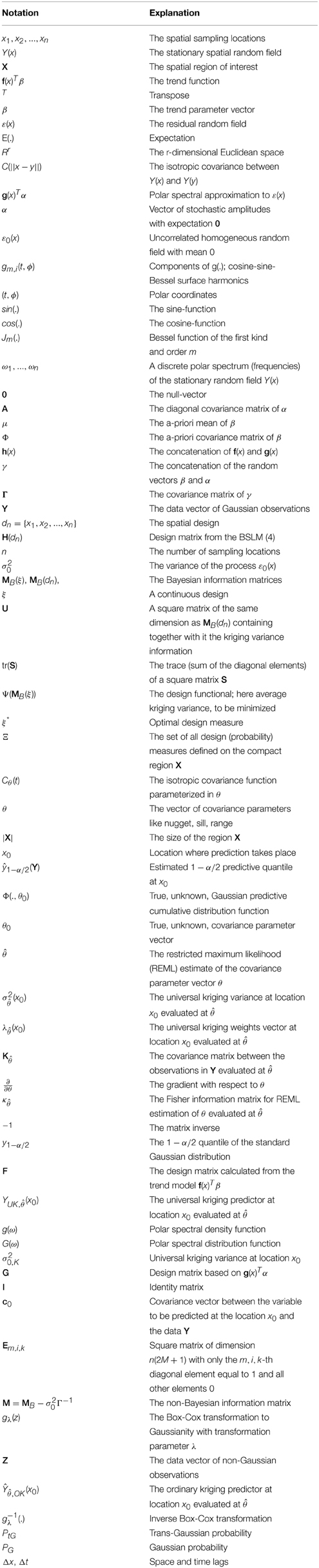
Table 1. Notations sorted in order of appearance.

Now, combining (Equations 1–3), we arrive at the Bayesian spatial linear model (BSLM)

$\begin{array}{ll}Y(x)=h{(x)}^T\gamma +{\epsilon }_0(x)\hfill & (4)\hfill \end{array}$

where

$\begin{array}{l}h(x)=\left(\begin{array}{c}f(x)\\ g(x)\end{array}\right),\gamma =\left(\begin{array}{c}\beta \\ \alpha \end{array}\right),\\ \text{E}(\gamma )=\left(\begin{array}{c}\mu \\ 0\end{array}\right),\text{Cov}(\gamma )=\left(\begin{array}{c}\Phi 0\\ 0A\end{array}\right)=:\Gamma \end{array}$

Here A is a diagonal covariance matrix containing as variance components either 1-times or 2-times the heights of the steps of the step-wise approximation to the polar spectral distribution function (see also, Equation 12). Spöck and Pilz (2010) demonstrate that Bayesian linear trend estimation in the above BSLM actually approximates Bayesian linear kriging in the original model arbitrarily closely. The same is true for the total mean squared error (TMSEP) of the trend prediction and the TMSEP of Bayesian kriging. The BSLM Equation (4) is an accurate substitute for the original random field if its isotropic covariance function C(||x₁ − x₂||) is well-approximated by the non-stationary covariance function C(x₁, x₂) = g(x₁)^T Ag(x₂) of the BSLM. See Section 7 and Figure 5 how much accuracy is possible with 3094 cosine-sine-Bessel surface harmonics.

Taking the TMSEP

${\sigma }_0^2\{1+h{(x_0)}^T{(H^{T}H+{\sigma }_0^2{\Gamma }^{-1})}^{-1}h(x_0)\}$

of the Bayesian spatial linear trend prediction

$h{(x_0)}^T{(H^{T}H+{\sigma }_0^2{\Gamma }^{-1})}^{-1}(H^{T}Y+{\sigma }_0^2{\Gamma }^{-1}{\gamma }_0)$

in the approximating BSLM as a substitute for the original Bayes kriging TMSEP, we arrive at the following classical experimental design problem for so-called I-optimality:

$\begin{array}{ll}\begin{array}{l}{\displaystyle {\int }_{X}h}{(x_0)}^T{(H^T(d_n)H(d_n)+{\sigma }_0^2{\Gamma }^{-1})}^{-1}h(x_0)d{x}_0\\ \to \underset{d_n}{\min }.\end{array}\hfill & (5)\hfill \end{array}$

Here “I” is a substitute for “Integrated”: The integral of the TMSEPs is calculated over the whole region of investigation X and then optimal design locations are searched for in such a way that this integral becomes minimized. d_n = {x₁, x₂, …, x_n} collects either the design points to be added to the monitoring network or in the case of reducing the network the design points remaining in the monitoring network. H(d_n) = (h_j(x_i))_i,j denotes the design matrix, which explicitly depends on the design points in the set d_n and Y = (Y(x₁), …, Y(x_n))^T is the vector of available data.

At this point we advise the reader not familiar with Bayesian experimental design theory to read the Appendix of Spöck and Pilz (2010). It is appropriate to clarify here just the statistical difference between experimental design and spatial sampling design: Spatial sampling design tries to specify in an optimal way measurement locations of a spatial process in order to predict it optimally or to make optimal estimates of its properties. Experimental design on the other hand is related to the planning of experiments, especially in combination with regression- or analysis of variance models. Concerning regression- and analysis of variance models the key point in this theory is that the above so-called concrete design problem, which is mathematically intractable, may be expanded to a so-called continuous design problem that has the nice feature of being a convex optimization problem. Thus, the whole apparatus of convex optimization theory is available to approximately solve the above design problem for I-optimality. In particular, directional derivatives may be calculated and optimal continuous designs may be found by steepest descent algorithms. Continuous designs are just probability measures ξ on X and may be rounded to exact designs d_n. Defining the so-called continuous Bayesian information matrix

$\begin{array}{ll}{M}_B(\xi )={\displaystyle {\int }_{X}h(x)h{(x)}^T\xi (dx)+\frac{{\sigma }_0^2}{n}{\Gamma }^{-1}}\hfill & (6)\hfill \end{array}$

and

$\begin{array}{ll}U={\displaystyle {\int }_{X}h(x_0)h{(x_0)}^{T}d{x}_0},\hfill & (7)\hfill \end{array}$

it may be shown that the set of all such information matrices is convex and compact and that the extended design functional

$\begin{array}{ll}\Psi (M_B(\xi ))=\text{tr}(U{M}_B{(\xi )}^{-1})\hfill & (8)\hfill \end{array}$

is convex and continuous in M_B(ξ). The above design functional Ψ(.) thus attains its minimum at a design ξ* ∈ Ξ, where Ξ is the set of all probability measures defined on the compact design region X, see (Pilz, 1991). The closeness of exact designs d_n to the optimal continuous design ξ* may be judged by means of a well-known efficiency formula (cp. the Appendix of Spöck and Pilz, 2010).

The idea to approximate the random field by a linear mixed model containing a linear deterministic trend component plus a linear stochastic fluctuation component of the form Equation (1) is not new. Actually, Fedorov (1996) was the first to do this. He made use of the so-called Karhunen-Loeve approximation to the error process. This approach has the disadvantage that a complicated Eigen-problem has to be solved, whereas the calculation of the polar spectral approximation, which is used here, is easier and more accessible, see (Spöck and Pilz, 2010). We also think that there is not much accuracy lost in combination with computation time in using the polar spectral representation although it is true for sure that the Karhunen-Loeve representation makes use of Eigen-functions and therefore should provide more accuracy with the same number of surface harmonics. Up to date we have no numerical experience in this direction because of the complicatedness of the Eigen-problems to be solved.

The real problem with spatial sampling design is that it is a complicated combinatorial task to select a certain number of measurement locations in an optimal way to minimize certain criteria concerning optimality of prediction or estimation of certain properties of the random field. Up to date the most used methodology to optimize these criteria and select measurement locations in an optimal way is simulated annealing, Groenigen et al. (1999). Simulated annealing has the disadvantage that it is random, slow, very time consuming and that different restarts of the algorithm lead to different results. On the opposite, our approach, showing the equivalence of the spatial sampling design problem to an experimental design problem from Bayesian linear regression, can be solved by means of deterministic steepest descent algorithms and even more, spatial sampling designs can be characterized using experimental design theory by means of well-known equivalence theorems, Kiefer (1959), Fedorov (1972), and Whittle (1973).

3. The Smith and Zhu Design Criterion Taking Account of Estimated Covariance Function

In real world applications the isotropic covariance function C_θ(t) is always uncertain and has to be estimated. The kriging predictor used is then based on this estimated covariance function. Thus, the kriging predictor is always a plug-in predictor with the estimate for the covariance function inserted into the formula for the kriging predictor and the reported (plug-in) kriging variance may be shown to underestimate the true variance of this plug-in predictor, Harville and Jeske (1992).

Smith and Zhu (2004) consider spatial sampling design by means of minimizing the average of the lengths of estimated 1 − α predictive intervals:

$\begin{array}{l}\frac{1}{\left|X\right|}{\displaystyle {\int }_X\{\text{length of estimated}1-\alpha \text{predictive}}\\ \text{interval at }{x}_0\}d{x}_0\to \underset{d_n=\{x_1,\dots ,x_n\}}{Min}\end{array}$

Here |X| denotes the area of the design region. Their predictors of the α/2 and 1 − α/2 quantiles of the predictive distributions are selected in such a way that the corresponding estimated predictive intervals have coverage probability bias 0 to order O(n⁻¹), where n is the number of observations. That means, E{Φ(ŷ_1−α/2(Y), θ₀)} = 1 − α/2 to order O(n⁻¹), where ŷ_1−α/2(Y) is the estimated (1 − α/2) predictive quantile and Φ(., θ₀) is the true, unknown predictive cumulative distribution function, i.e., a Gaussian distribution with mean equal to the true unknown universal kriging predictor and variance equal to the true unknown universal kriging variance, both based on the true unknown covariance parameters θ₀. The above expectation is taken with respect to the true unknown Gaussian distribution of the data Y. The estimates ŷ_α/2(Y) and ŷ_1−α/2(Y) of the mentioned quantiles are essentially the plug-in universal kriging predictor based on restricted maximum likelihood (REML) estimation of the covariance parameters ± a scaled plug-in kriging standard deviation term that is corrected to take account of REML estimation, see Equation (35) and (Smith and Zhu, 2004). Based on Laplace approximations of the true and estimated predictive densities and on second-order Taylor expansions of some more expressions, Smith and Zhu (2004) show that the above design criterion, up to order O(n⁻²), is equivalent to:

$\begin{array}{ll}\begin{array}{l}{\int }_X[{\sigma }_{\widehat{\theta }}^2(x_0)+\text{tr}({\kappa }_{\widehat{\theta }}^{-1}{\{\frac{\partial {\lambda }_{\widehat{\theta }}(x_0)}{\partial {\theta }^T}\}}^T{K}_{\widehat{\theta }}\frac{\partial {\lambda }_{\widehat{\theta }}(x_0)}{\partial {\theta }^T})\\ +y_{1-\alpha /2}^2{\{\frac{\partial {\sigma }_{\widehat{\theta }}(x_0)}{\partial \theta }\}}^T{\kappa }_{\widehat{\theta }}^{-1}\frac{\partial {\sigma }_{\widehat{\theta }}(x_0)}{\partial \theta }]d{x}_0\\ \to \underset{d_n=\{x_1,\dots ,x_n\}}{Min}\end{array}\hfill & (9)\hfill \end{array}$

Obviously the above design functional is evaluated at $\widehat{\theta }$, the REML estimate of the covariance parameters. Above

$\begin{array}{ll}{({\kappa }_{\widehat{\theta }})}_{i,j}=\text{tr}(W_{\widehat{\theta }}\frac{\partial K_{\widehat{\theta }}}{\partial {\theta }_i}{W}_{\widehat{\theta }}\frac{\partial K_{\widehat{\theta }}}{\partial {\theta }_j})\hfill & (10)\hfill \end{array}$

is the Fisher information matrix for REML estimation of θ,

$\begin{array}{ll}{W}_{\widehat{\theta }}=K_{\widehat{\theta }}^{-1}-K_{\widehat{\theta }}^{-1}F{(F^T{K}_{\widehat{\theta }}^{-1}F)}^{-1}{F}^T{K}_{\widehat{\theta }}^{-1},\hfill & (11)\hfill \end{array}$

y_1−α/2 is the 1−α/2-quantile of the standard normal distribution, σ²_{$\widehat{\theta }$}(x₀) is the universal kriging variance at x₀ and λ_{$\widehat{\theta }$}(x₀) is the universal kriging weights vector for prediction at x₀ so that the universal plug-in kriging predictor reads

$Y_{UK,\widehat{\theta }}(x_0)={\lambda }_{\widehat{\theta }}{(x_0)}^{T}Y$

The design criterion given above takes both prediction accuracy and covariance uncertainty into account. A design criterion similar to the Smith and Zhu (2004) criterion was considered also by Zimmerman (2006).

Some details on the derivation of the above Equation (9) are indicated here: Laplace-approximation tries to approximate the value of the integral

${\displaystyle {\int }_{\Theta }{e}^{l(\theta )+Q(\theta )}}\Psi (y_p;Y,\theta )d\theta$

Actually, the Bayesian predictive density at a location x₀ can be written as a quotient of two such expressions with l(θ) the restricted log-likelihood function, Ψ(y_p; Y, θ) the Gaussian distribution function having as mean the universal kriging predictor at x₀ and as variance the universal kriging variance and Q(θ) the log of the a-priori density for θ. Laplace-approximation approximates the function l(θ) + Q(θ) + log(Ψ(y_p; Y, θ*)) by a second-order Taylor expansion at θ* with θ* either the true unknown covariance parameter θ₀, its REML-estimate $\widehat{\theta }$ or its posterior mode θ_M and then calculates an approximation to the above integral as

${\{\frac{2\pi }{n}\}}^{p/2}|{\Sigma }_{{\theta }^{\ast }}{|}^{-1/2}{e}^{l({\theta }^{\ast })+Q({\theta }^{\ast })}\Psi (y_p;Y,{\theta }^{*}),$

where p is the dimension of θ, n is the number of data and ${\Sigma }_{{\theta }^{\ast }}=\frac{{\partial }^2\frac{1}{n}(l({\theta }^{\ast })+Q({\theta }^{\ast })+\text{log}(\Psi (y_p;Y,{\theta }^{*})))}{\partial \theta \partial {\theta }^T}$ is the Hessian of $\frac{1}{n}(l({\theta }^{\ast })+Q({\theta }^{\ast })+\text{log}(\Psi (y_p;Y,{\theta }^{\ast })))$. Further simplifications in the derivation of the above Equation (9) are made by means of applying further second-order Taylor approximations to the inverse Gaussian distribution function Ψ⁻¹(.; Y, θ) at θ*.

4. Experimental Design Theory Applied to the Smith and Zhu Design Criterion

Sections 2, 3 have demonstrated that by using the BSLM (Equation 4) as approximation to the true isotropic random field the I-optimality design criterion (Equation 5) can be completely expressed in terms of the Bayesian information matrix

$M_B=H^{T}H+{\sigma }_0^2{\Gamma }^{-1}.$

and that it is convex on the set of all such information matrices. Thus, classical convex experimental design algorithms could be used to find optimal spatial sampling designs minimizing the criterion (Equation 5).

The aim of this section is to demonstrate that the (Smith and Zhu, 2004) design criterion has some favorable properties, too, which allow the application of classical convex experimental design theory to this design criterion:

Theorem: Expression (Equation 9) can be expressed completely in terms of the Bayesian information matrix M_B. The design functional is continuous on the convex and compact set of all matrices M_B(ξ).

This allows us to make use of classical iterative experimental design algorithms to find spatial sampling designs. The next following Subsection proves the stated Theorem.

4.1. Proof that the Smith-Zhu Design Criterion can be Expressed Completely in terms of the Bayesian Information Matrix M_B

Assuming the BSLM (Equation 4), the covariance function actually is parameterized through the diagonal matrix A and the nugget variance σ²₀. Since the (Smith and Zhu, 2004) design criterion assumes the covariance parameters to be estimated by REML we actually estimate this diagonal matrix A and σ²₀ by this methodology. The a priori covariance matrix Φ = Cov(β) must be given almost infinite diagonal values because the (Smith and Zhu, 2004) approach assumes the trend parameter vector β to be estimated by generalized least squares and Φ → ∞ bridges the gap from Bayesian linear to generalized least squares trend estimation. The a priori mean μ = E(β) can be set to 0 then.

According to the polar spectral representation given in Spöck and Pilz (2010), several values in the diagonal matrix A are identical:

$\begin{array}{ll}\begin{array}{l}A=\text{diag}({\left\{d_m{a}_i^2\right\}}_{m=0_k^{\ast },\dots ,M;i=1,\dots ,n;k=1,2}),\\ \text{with }{0}_k^{\ast }=0\text{if }k=1\text{and }{0}_k^{\ast }=1\text{else},\end{array}\hfill & (12)\hfill \end{array}$

where the definitions of the a²_i's, -the discrete spectra-, and the indexing derive from the polar spectral representation given in Spöck and Pilz (2010). k = 1, 2 index the sine-Bessel term and the cosine-Bessel term in formula (Equation 2), respectively d_m = 1 for m = 0 and d_m = 2 for m ≥ 1. For REML estimation of A we have two possibilities:

• We can leave the discrete spectra a²_i unspecified: This approach is almost non-parametric because a lot of a_i's and corresponding frequencies w_i are needed to get the isotropic random field properly approximated and corresponds to a semiparametric estimation of the spectral distribution function via a step function.

• We can specify a parametric model for the a²_i's: The polar spectral density function for an isotropic random field over R² possessing for example an exponential covariance function $B(h)=C\text{exp}(-\frac{3h}{\alpha })$ is given by

$g(w)=\frac{C\frac{3}{\alpha }w}{{\left({(\frac{3}{\alpha })}^2+w^2\right)}^{3/2}}.$

We note that this α for the range is different from the α in Equation (1). The polar spectral density function is defined as the first derivative of the polar spectral distribution function G(w), see (Spöck and Pilz, 2010). A possible parametrization for the a²_i's:

$\begin{array}{ll}\begin{array}{l}{a}_i^2=0.5(g(w_i)+g(w_{i-1}))(w_i-w_{i-1}),\\ i=1,2,\dots ,n,\end{array}\hfill & (13)\hfill \end{array}$

where 0 = w₀ < w₁ < … < w_n are fixed frequencies.

Figure 1 displays the behavior of different types of correlation functions and their associated polar spectral distribution functions. The approximations of the correlation functions are based on 50 pre-specified support points ω₁, …, ω₅₀ with increasing frequency lags. The approximations for the spherical and exponential correlation functions are close enough even for 30 and fewer support points. Roughly speaking, if the correlation function C(r)/C(0) is suspected to have a steep descent at the origin (irregular behavior and strong fluctuations of Y(.)) then ω_n should be chosen large enough, whereas in case of a more regular behavior of Y(.) and moderate steepness of the correlation function near the origin (as e.g., in case of a Gaussian correlation function) we do not need large frequencies ω_n. The relationship between the gradient of the correlation function at the origin and the choice of the largest necessary frequency ω_n can be more deeply explored using results from Yaglom (1987), especially results 4.1.46 and 4.1.47. From our numerical experience we propose to choose ω_n > ω_0.99, the 99%-quantile of the spectral distribution function [99% of its maximum level C(+0)], i.e., G(ω_0.99) = 0.99C(+0). For example, for a Gaussian covariance function C(r) = s exp(3r²/ α²) with sill s = 1 and range α = 10, we obtain ω_0.99 = 0.825, whereas for a spherical covariance function with the same parameters we obtain ω_0.99 = 19.5.

FIGURE 1

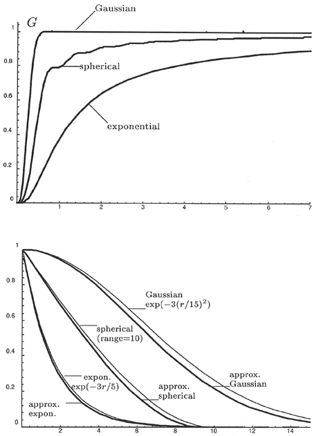
Figure 1. Above: Polar spectral distribution functions. Below: Corresponding correlation functions and their approximations.

One may want to skip the following subsubsections at a first reading. It is just shown there that the (Smith and Zhu, 2004) design criterion can be expressed as a function of the information matrix M_B.

4.1.1. Proof that the Kriging Variance σ²_0,K, the Kriging Weights Vector λ and W can be Expressed in Terms of M_B

According to Equation (5), the kriging variance can be expressed as

${\sigma }_{0,K}^2={\sigma }_0^2\left(1+h{(x_0)}^T{M}_B^{-1}h(x_0)\right).$

The kriging weights vector may be written

$\lambda =H{M}_B^{-1}h(x_0),$

and furthermore,

$\begin{array}{ll}W=\frac{1}{{\sigma }_0^2}(I-H{M}_B^{-1}{H}^T),\hfill & (14)\hfill \end{array}$

where I is the identity matrix. All these expressions derive from the application of the Sherman-Morrison-Woodbury matrix inversion formula

$\begin{array}{l}{(A+UCV)}^{-1}=\\ =A^{-1}-A^{-1}U{(C^{-1}+V{A}^{-1}U)}^{-1}V{A}^{-1},\end{array}$

from the fact that GAg(x₀) and σ²₀I + GAG^T are the vector of covariances and covariance matrix of observations, respectively, and that the kriging weights vector for Bayesian kriging may be written as

$\lambda ={(K+F\Phi F^T)}^{-1}(c_0+F\Phi f(x_0)),$

where F is the design matrix of the linear regression that is based on the drift function f(x).

4.1.2. Partial derivatives of M⁻¹_B

Let M_B = H^T H + σ²₀Γ⁻¹ be the Bayesian information matrix. Using the matrix identity

$\frac{\partial M^{-1}}{\partial t}=-M^{-1}\frac{\partial M}{\partial t}{M}^{-1},$

the partial derivative of M⁻¹_B with respect to σ²₀ = nugget may be calculated as

$\begin{array}{ll}\frac{\partial M_B^{-1}}{\partial {\sigma }_0^2}=-M_B^{-1}{\Gamma }^{-1}{M}_B^{-1}.\hfill & (15)\hfill \end{array}$

Defining

$\begin{array}{l}{\gamma }_{m,i,k}=d_m{a}_i^2,\\ m=0_k^{\ast },\dots ,M;\\ i=1,\dots ,n;\\ k=1,2\end{array}$

we obtain

$\frac{\partial M_B^{-1}}{\partial {\gamma }_{m,i,k}}=\frac{{\sigma }_0^2}{{\gamma }_{m,i,k}^2}{M}_B^{-1}{E}_{m,i,k}{M}_B^{-1},$

where E_m,i,k is a matrix of 0's, with only the m, i, k-th diagonal element being 1. Setting γ_m,i,k = d_ma²_i and using

$\frac{\partial M_B^{-1}}{\partial a_i^2}={\displaystyle \sum _{k=1,2}{\displaystyle \sum _{m=0_k^{\ast }}^M\frac{\partial M_B^{-1}}{\partial {\gamma }_{m,i,k}}}\frac{\partial {\gamma }_{m,i,k}}{\partial a_i^2}}$

one gets

$\begin{array}{ll}\frac{\partial M_B^{-1}}{\partial a_i^2}=\frac{{\sigma }_0^2}{a_i^4}{M}_B^{-1}{J}_i{M}_B^{-1},\hfill & (16)\hfill \end{array}$

where

$J_i={\displaystyle \sum _{k=1,2}{\displaystyle \sum _{m=0_k^{\ast }}^M\frac{1}{d_m}{E}_{m,i,k}}}.$

For the parametric model (Equation 13), partial derivatives with respect to α = range, C = partial sill may be calculated by using

$\begin{array}{l}\frac{\partial M_B^{-1}}{\partial \alpha }={\displaystyle \sum _{i=1}^n\frac{\partial M_B^{-1}}{\partial a_i^2}}\frac{\partial a_i^2}{\partial \alpha }\\ \frac{\partial M_B^{-1}}{\partial C}={\displaystyle \sum _{i=1}^n\frac{\partial M_B^{-1}}{\partial a_i^2}}\frac{\partial a_i^2}{\partial C}.\end{array}$

Defining

$\begin{array}{l}{J}_{\alpha }={\sigma }_0^2{\displaystyle \sum _{i=1}^n\frac{1}{a_i^4}\frac{\partial a_i^2}{\partial \alpha }{J}_i},\\ J_C={\sigma }_0^2{\displaystyle \sum _{i=1}^n\frac{1}{a_i^4}\frac{\partial a_i^2}{\partial C}{J}_i}\end{array}$

one obtains

$\begin{array}{ll}\frac{\partial M_B^{-1}}{\partial \alpha }=M_B^{-1}{J}_{\alpha }{M}_B^{-1}\hfill & (17)\hfill \end{array}$

$\begin{array}{ll}\frac{\partial M_B^{-1}}{\partial C}=M_B^{-1}{J}_C{M}_B^{-1}\hfill & (18)\hfill \end{array}$

Note, these expressions are dependent on the spatial design only via the Bayesian information matrix M_B.

4.1.3. Partial Derivatives of σ_0,K and λ

Using the partial derivatives of M⁻¹_B given in Section 4.1.2 and the expressions for σ²_0,K and λ from Section 4.1.1, we arrive at:

$\begin{array}{ll}\frac{\partial {\sigma }_{0,K}^2}{\partial {\sigma }_0^2}=1+\text{tr}(h(x_0)h{(x_0)}^T{M}_B^{-1}M{M}_B^{-1})\hfill & (19)\hfill \end{array}$

$\begin{array}{ll}\frac{\partial \lambda }{\partial {\sigma }_0^2}=-H{M}_B^{-1}{\Gamma }^{-1}{M}_B^{-1}h(x_0)\hfill & (20)\hfill \end{array}$

$\begin{array}{ll}\begin{array}{l}\frac{\partial {\sigma }_{0,K}^2}{\partial a_i^2}=\frac{{\sigma }_0^4}{a_i^4}\text{tr}(h(x_0)h{(x_0)}^T{M}_B^{-1}{J}_i{M}_B^{-1})\\ \frac{\partial \lambda }{\partial a_i^2}=\frac{{\sigma }_0^2}{a_i^4}H{M}_B^{-1}{J}_i{M}_B^{-1}h(x_0)\end{array}\hfill & (21)\hfill \end{array}$

$\begin{array}{ll}\frac{\partial {\sigma }_{0,K}^2}{\partial \alpha }={\sigma }_0^2\text{tr}(h(x_0)h{(x_0)}^T{M}_B^{-1}{J}_{\alpha }{M}_B^{-1})\hfill & (22)\hfill \end{array}$

$\begin{array}{ll}\begin{array}{l}\frac{\partial {\sigma }_{0,K}^2}{\partial C}={\sigma }_0^2\text{tr}(h(x_0)h{(x_0)}^T{M}_B^{-1}{J}_C{M}_B^{-1})\\ \frac{\partial \lambda }{\partial \alpha }=H{M}_B^{-1}{J}_{\alpha }{M}_B^{-1}h(x_0)\end{array}\hfill & (23)\hfill \end{array}$

$\begin{array}{ll}\frac{\partial \lambda }{\partial C}=H{M}_B^{-1}{J}_C{M}_B^{-1}h(x_0),\hfill & (24)\hfill \end{array}$

where M = M_B − σ²₀Γ⁻¹. Partial derivatives $\frac{\partial {\sigma }_{0,K}}{\partial \theta }$ are then given as

$\begin{array}{ll}\frac{\partial {\sigma }_{0,K}}{\partial \theta }=\frac{\partial {\sigma }_{0,K}^2}{\partial \theta }/(2\sqrt{{\sigma }_{0,K}^2}).\hfill & (25)\hfill \end{array}$

4.1.4. Proof that the Information Matrix κ can be Expressed in Terms of M_B

The i, j-th element of the information matrix κ is defined in Equation (10), where W is defined in Equation (14) and we must set

$\begin{array}{ll}K=H\Gamma H^T+{\sigma }_0^{2}I-F\Phi F^T.\hfill & (26\hfill \end{array})$

In the semiparametric model θ_i and θ_j are either made of the parameters a_i, a_j, σ²₀; for the parametric model θ_i and θ_j may be either made of the parameters α, C, σ²₀.

For the partial derivatives of K we obtain along the same lines of reasoning as in Sections 4.1.2, 4.1.3:

$\begin{array}{l}\frac{\partial K}{\partial {\sigma }_0^2}=I\\ \frac{\partial K}{\partial a_i^2}=H{L}_i{H}^T\\ \frac{\partial K}{\partial \alpha }=H{L}_{\alpha }{H}^T\\ \frac{\partial K}{\partial C}=H{L}_C{H}^T,\end{array}$

where

$\begin{array}{l}{L}_i={\displaystyle \sum _{k=1,2}{\displaystyle \sum _{m=0_k^{\ast }}^M{d}_m{E}_{m,i,k}}},\\ L_{\alpha }={\displaystyle \sum _{i=1}^n\frac{\partial a_i^2}{\partial \alpha }{L}_i},\\ L_C={\displaystyle \sum _{i=1}^n\frac{\partial a_i^2}{\partial C}{L}_i}.\end{array}$

Inserting these expressions and the expression (Equation 14) for W into the definition (Equation 10) of the Fisher information matrix we obtain, after some linear algebra, the following expressions for κ:

$\begin{array}{ll}{\kappa }_{a_i^2,a_j^2}=\text{tr}(L_{j}V{L}_{i}V)\hfill & (27)\hfill \end{array}$

$\begin{array}{ll}\begin{array}{l}{\kappa }_{{\sigma }_0^2,{\sigma }_0^2}=\frac{n-m}{{\sigma }_0^4}+\text{tr}({\Gamma }^{-1}{M}_B^{-1}{\Gamma }^{-1}{M}_B^{-1})\\ {\kappa }_{{\sigma }_0^2,a_i^2}=\text{tr}({\Gamma }^{-1}{M}_B^{-1}V{L}_i)\\ {\kappa }_{\alpha ,\alpha }=\text{tr}(L_{\alpha }V{L}_{\alpha }V)\end{array}\hfill & (28)\hfill \end{array}$

$\begin{array}{ll}{\kappa }_{C,C}=\text{tr}(L_{C}V{L}_{C}V)\hfill & (29)\hfill \end{array}$

$\begin{array}{ll}{\kappa }_{\alpha ,C}=\text{tr}(L_{C}V{L}_{\alpha }V)\hfill & (30)\hfill \end{array}$

$\begin{array}{ll}{\kappa }_{{\sigma }_0^2,\alpha }=\text{tr}({\Gamma }^{-1}{M}_B^{-1}V{L}_{\alpha })\hfill & (31)\hfill \end{array}$

$\begin{array}{ll}{\kappa }_{{\sigma }_0^2,C}=\text{tr}({\Gamma }^{-1}{M}_B^{-1}V{L}_C),\hfill & (32)\hfill \end{array}$

where

$V={\Gamma }^{-1}-{\sigma }_0^2{\Gamma }^{-1}{M}_B^{-1}{\Gamma }^{-1},$

n is the number of design locations and m is the dimension of the information matrix.

4.1.5. The Smith-Zhu Design Criterion Expressed Completely in Terms of M_B

We are now going to show that the (Smith and Zhu, 2004) design criterion (Equation 9) is dependent on the spatial sampling design only via the Bayesian information matrix M_B. For simplicity we consider here only the expression of this design criterion for the parametric model (Equation 13). By analogy, similar expressions may be derived also for the semiparametric model. Defining

θ = (σ²₀, α, C)^T we have to derive expressions for

$\text{tr}\left({\kappa }^{-1}{\{\frac{\partial \lambda }{\partial {\theta }^T}\}}^{T}K\frac{\partial \lambda }{\partial {\theta }^T}\right)$

and

${\{\frac{\partial {\sigma }_{0,K}}{\partial \theta }\}}^T{\kappa }^{-1}\frac{\partial {\sigma }_{0,K}}{\partial \theta }.$

Expressions dependent only on M_B for the 3 × 3 matrix κ, for the kriging variance σ²_0,K and all partial derivatives of σ_0,K and λ have already been given in the last subsubsections.

Defining the 3-column matrix

$\begin{array}{l}{R}_{x_0}=(-M_B^{-1}{\Gamma }^{-1}{M}_B^{-1}h(x_0),\\ M_B^{-1}{J}_{\alpha }{M}_B^{-1}h(x_0),M_B^{-1}{J}_C{M}_B^{-1}h(x_0))\end{array}$

such that

$\frac{\partial \lambda }{\partial {\theta }^T}=H{R}_{x_0}$

we obtain after some linear algebra

$\begin{array}{ll}\begin{array}{l}\text{tr}\left({\kappa }^{-1}{\{\frac{\partial \lambda }{\partial {\theta }^T}\}}^{T}K\frac{\partial \lambda }{\partial {\theta }^T}\right)=\\ =\text{tr}\left({\kappa }^{-1}{R}_{x_0}{}^T\{MUM+{\sigma }_0^{2}M\}{R}_{x_0}\right),\end{array}\hfill & (33)\hfill \end{array}$

where

$\begin{array}{l}M=M_B-{\sigma }_0^2{\Gamma }^{-1}\\ U=\left(\begin{array}{c}00\\ 0A\end{array}\right).\end{array}$

Obviously,

$\begin{array}{ll}{\{\frac{\partial {\sigma }_{0,K}}{\partial \theta }\}}^T{\kappa }^{-1}\frac{\partial {\sigma }_{0,K}}{\partial \theta }\hfill & (34)\hfill \end{array}$

is dependent on the spatial design only via the Bayesian information matrix M_B, observing expressions (Equations 27–32) for κ and the expressions (Equations 20–25) for the partial derivatives of σ_0,K.

We may now consider experimental design ideas and replace, in the above expressions for the (Smith and Zhu, 2004) design criterion, the matrix M_B everywhere by its continuous version nM_B(ξ), where n is the number of spatial samples in consideration and

$M_B(\xi )={\displaystyle {\int }_{X}h(x)h{(x)}^T\xi (dx)}+\frac{{\sigma }_0}{n}{\Gamma }^{-1}$

with ξ(dx) a probability measure on the design space X, is the so-called continuous Bayesian information matrix associated to the BSLM (Equation 4). As already mentioned, the set of all such information matrices is convex and compact. This way the (Smith and Zhu, 2004) design criterion becomes a continuous functional over the convex and compact set of all such continuous Bayesian information matrices M_B(ξ). Continuity and compactness are nice properties because they guarantee that actually a minimum among all such continuous information matrices exists for this design functional.

5. Spatial Sampling Design for Trans-Gaussian Kriging

In trans-Gaussian kriging the originally positive valued data Z(x_i), i = 1, 2, …, n are transformed to Gaussianity by means of the Box-Cox-transformation

$g_{\lambda }(z)=\{\begin{array}{c}\frac{z^{\lambda }-1}{\lambda }:\lambda \cancel{=}0\\ \text{log}(z):\lambda =0\end{array}.$

Let Z = (Z(x₁), Z(x₂), …, Z(x_n))^T be the vector of original data and

$Y={(g_{\lambda }(Z(x_1)),g_{\lambda }(Z(x_2)),\dots ,g_{\lambda }(Z(x_n)))}^T$

be the vector of transformed data. The predictive density for trans-Gaussian kriging at a location x₀ then may be written:

$\phi (g_{\lambda }(z);{\widehat{Y}}_{OK}(x_0),{\sigma }_{OK}^2(x_0))z^{\lambda -1},$

where φ(.; Ŷ_OK(x₀), σ²_OK(x₀)) is the Gaussian density with mean equal to the ordinary kriging predictor Ŷ_OK(x₀) at x₀ and based on the transformed variables Y, and variance equal to the ordinary kriging variance σ²_OK(x₀). The expression z^λ−1 is the Jacobian of the Box-Cox transformation.

For spatial sampling design taking into account the REML estimation of the covariance parameters θ we can consider again the average of the lengths of estimated (1 − α)-predictive intervals. In order to make the lengths of estimated predictive intervals also dependent on REML-estimation of the covariance function, we can consider instead of the Gaussian density φ(. ; Ŷ_OK(x₀), σ²_OK(x₀)) that unique Gaussian density whose α/2 and 1 − α/2 quantiles are given by the endpoints of the following estimated (1 − α) predictive interval derived in Smith and Zhu (2004) and having coverage probability bias 0 to order O(n⁻¹):

$\begin{array}{ll}\begin{array}{l}{\widehat{Y}}_{\widehat{\theta },OK}(x_0)\pm \\ y_{1-\alpha /2}{\sigma }_{\widehat{\theta }}(x_0)\{1+\\ \frac{1}{2{\sigma }_{\widehat{\theta }}^2(x_0)}[\text{tr}({\kappa }_{\widehat{\theta }}^{-1}{\{\frac{\partial {\lambda }_{\widehat{\theta }}(x_0)}{\partial {\theta }^T}\}}^T{K}_{\widehat{\theta }}\frac{\partial {\lambda }_{\widehat{\theta }}(x_0)}{\partial {\theta }^T})+\\ y_{1-\alpha /2}^2{\{\frac{\partial {\sigma }_{\widehat{\theta }}(x_0)}{\partial \theta }\}}^T{\kappa }_{\widehat{\theta }}^{-1}\frac{\partial {\sigma }_{\widehat{\theta }}(x_0)}{\partial \theta }]\}.\end{array}\hfill & (35)\hfill \end{array}$

Here, $\widehat{\theta }$ is the REML estimate of the covariance parameters and all expressions are evaluated at this estimate, y_1−α/2 is the 1 − α/2 quantile of the standard normal distribution.

Later, when calculating spatial sampling designs with the algorithms from the Appendix and investigating new prospective design locations with no data available, we have to replace in the statistic T_{$\widehat{\theta }$}(Y) = Ŷ_{$\widehat{\theta }$, OK}(x₀) every variable Y(x_i) for which we do not have a datum by its ordinary kriging predictor based on the available data.

The above estimated lower and upper quantiles ŷ_α/2 and ŷ_1−α/2 of the Gaussian estimated 1 − α predictive intervals are transformed back to the original Z-scale by means of the inverse Box-Cox transformation g⁻¹_λ(.) to get estimated predictive intervals

$[{\widehat{z}}_{\alpha /2}:=g_{\lambda }^{-1}({\widehat{y}}_{\alpha /2}),{\widehat{z}}_{1-\alpha /2}:=g_{\lambda }^{-1}({\widehat{y}}_{1-\alpha /2})]$

for trans-Gaussian kriging.

Moreover, although we have spoken only about the coverage probability bias 0 to order O(n⁻¹) of the estimated predictive intervals [ŷ_α/2, ŷ_{1 − α/2}] for Gaussian random fields, coverage probability bias 0 is also true for the proposed estimated trans-Gaussian predictive intervals [ž_α/2, ž_{1 − α/2}] as long as we consider the transformation parameter λ to be fixed and not estimated. This can be easily seen from the fact that

$\begin{array}{l}{P}_{tG}:=P_{tG}(Z_0\le {\widehat{z}}_{1-\alpha /2}|Z)=\\ =P_{tG}(g_{\lambda }(Z_0)\le g_{\lambda }({\widehat{z}}_{1-\alpha /2})|Z)=\\ =P_G(Y_0\le {\widehat{y}}_{1-\alpha /2}|Y)=:P_G,\end{array}$

where Z₀ and Z are random variables from the true trans-Gaussian random field and Y₀ and Y are random variables from the corresponding true Gaussian random field at locations x₀, x₁, …, x_n ∈ X, and g_λ(.) is the Box-Cox transformation. Thus, the random variables P_tG and P_G coincide. They provide the values of the true predictive trans-Gaussian and Gaussian distribution function at the estimated quantiles. For the Gaussian case we already know from the definition of ŷ_{1 − α/2} that E{P_G} = 1 − α/2 to order O(n⁻¹) because of unbiasedness. Here, again, the expectation is taken with respect to the true Gaussian distribution of the data Y. From the coincidence of the random variables P_tG and P_G we also have E{P_tG} = 1 − α/2 and the proposed estimated predictive intervals have thus coverage probability bias 0 also in the trans-Gaussian case.

In reality, the transformation parameter λ itself is estimated, too, e.g., by maximum likelihood, then is plugged-in into the ordinary kriging predictor Ŷ_{$\widehat{\theta }$, OK}(x₀) of (Equation 35) by means of transforming the original data Z with the estimated Box-Cox transformation, and is then used again to transform the Gaussian quantiles ŷ_α/2 and ŷ_{1 − α/2} by means of the inverse Box-Cox transformation to the original Z-scale. In a future paper we will take account of this additional uncertainty, assume that both λ and θ are estimated by means of maximum likelihood and will investigate estimated predictive intervals with coverage probability bias 0, too.

6. Properties of the Smith and Zhu Design Criterion and a Deterministic Optimization Algorithm

For the optimization of the (Smith and Zhu, 2004) design criterion we make use of the same principal greedy design algorithms as described in the Appendix. We must simply replace Ψ(ξ) from the Appendix by the (Smith and Zhu, 2004) design functional or the design functional for the trans-Gaussian case, both given by expressions (Equations 19–35) and the inverse Box-Cox-transformation. From these formulas it is obvious that in the Gaussian case, where the criterion (Equation 9) must be optimized, the calculation of the integral over the design region X appearing in Equation (9) can be simplified. Because all expressions under the integral sign are specific linear combinations of the components of the matrix function [h(x₀)h(x₀)^T] one just needs to compute the matrix U = ∫_Xh(x₀)h(x₀)^T dx₀ once, before applying the iterative design algorithms formulated in the Appendix. One then gets the integral (Equation 9) just by inserting components U_i,j from U instead of h_i(x₀)*h_j(x₀) in the expressions appearing in Equation (9) and referenced above.

At the first sight, no such computational simplification is possible for the trans-Gaussian case, since the components of [h(x₀)h(x₀)^T] enter the Gaussian quantiles (Equation 35) non-linearly through 1/σ²_{$\widehat{\theta }$}(x₀) and σ_{$\widehat{\theta }$}(x₀) and, moreover, these quantiles are transformed non-linearly via the inverse Box-Cox transformation. The design functional in the trans-Gaussian case may be written as the difference of two expressions having the form

$\begin{array}{l}{\displaystyle {\int }_X\text{inv}.\text{Box-Coxtransf}.\text{of}}\{\text{krigingpredictor}+\\ +\sqrt{\text{linear combination 1 of functions}}+\\ +\frac{\text{linear combination 2 of functions}}{\sqrt{\text{linear combination 1 of functions}}}\}d{x}_0\end{array}$

The functions referred to in the linear combinations are just the components of the matrix function h(x₀)h(x₀)^T. Thus, if one could show that integrals of the above form can be expressed just by the integrals of the component functions, then one could compute the above mentioned matrix U just before applying the design algorithms from the Appendix and the computational complexity during optimization would decrease a lot. Up to date, we could not show that the above mentioned simplification is possible. Therefore, in our implementation of the design algorithms given in the Appendix we have to compute an integral in every step of the optimization algorithms. This is computationally quite demanding as we will see in the following section, where we apply our ideas.

The proof of convexity properties of the (Smith and Zhu, 2004) design functional and the design functional for the trans-Gaussian case is a further topic for future research.

7. Network Design with Rainfall Data

Applications and numerical examples for the I-optimality design criterium of the Appendix have already been given in Spöck and Pilz (2010). There the so-called Gomel and Jura data sets have been considered. All the following computations are done with the MATLAB and Octave toolbox spatDesign:

wwwu.uni-klu.ac.at/guspoeck/
spatDesignMatlab.zip
wwwu.uni-klu.ac.at/guspoeck/
spatDesignOctave.zip

This toolbox is freely available from the first author.

7.1. Data Set and Preparatory Calculations

The data set considered here is a rainfall data set from Upper Austria, see (Mateu and Müller, 2012). The monitoring network comprises 36 locations. Total monthly rainfall has been measured at each location, starting in January 1994 and ending in December 2009. In Figure 2 we see that there are obviously areas in the design region that look very empty, having no sampling locations. Therefore, because it has only 36 monitoring stations and the correlation length of the covariance function, Figure 5, is relatively large compared to the design area, this data set is very suitable for spatial sampling design with the Smith-Zhu criterion. The variance of the covariance estimate is quite large and thus should be included in spatial sampling design. This is a situation that we are often confronted with in practical applications.

FIGURE 2

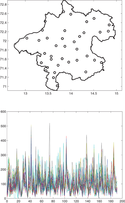
Figure 2. Above: The 36 sampling locations of the Upper Austria rainfall data set set. Below: The 36 time series of average monthly rainfall at each station.

In the book edited by Mateu and Müller (2012) this data set is analyzed by different authors with different methodologies. Different approaches to spatio-temporal design are developed there. Design locations are removed as well as added from/to the original design. The Smith-Zhu design criterion is considered by the authors of this article but also by second authors, Zimmerman and Lie (2013). Based on the Smith-Zhu criterion they remove two stations from the monitoring network, an approach that is computationally much less demanding than our approach of adding monitoring stations. The most common methodology used for optimization of the different design criteria in this book is simulated annealing, Aarts and Korst (1989). Besides integrated kriging variance (I-optimality) one other used design criterion in this book is entropy. It is also well-suited to be used in a Bayesian spatio-temporal approach to spatial sampling design. Furthermore, in the book also approaches to informative sampling and informative missingness are developed. Further chapters in Mateu and Müller (2012) pertain to large spatial-temporal data sets, improvements over random sampling, anisotropies in space-time kriging and sampling design, variable transformations and entropy criteria, adaptive-dynamic designs, dynamic designs in the non-Gaussian exponential family, machine learning and optimal design, pollution dispersion, and optimal design.

We now come back to our rainfall data set and calculate for each station the mean rainfall over the years, as well as the residual rainfall, for each of the 12 months, Figure 3. Hereafter, we calculate for each station the mean of standardized rain residuals, the empirical semivariogram corresponding to these means and a fitted exponential semivariogram to the means of original rain residuals, Figure 4.

FIGURE 3

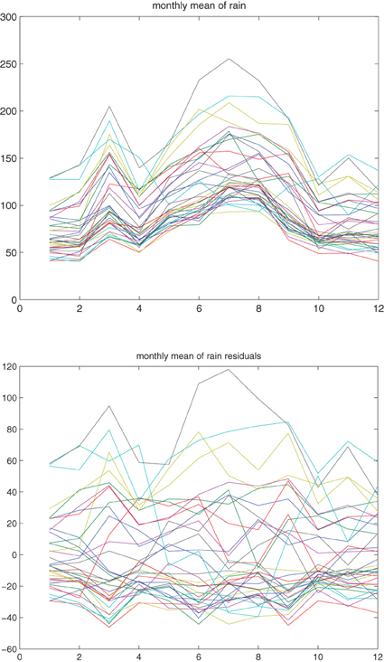
Figure 3. Above: The average monthly rainfall over the years at each of the 36 stations, for each of the 12 months. Below: The residual rainfall at each of the 36 stations, for each of the 12 months.

FIGURE 4

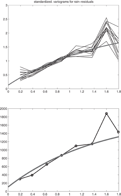
Figure 4. Above: Empirical semivariograms of the standardized rain residuals for all of the 12 months and a fitted exponential semivariogram (gray). Below: Empirical semivariogram for the means of original rain residuals and a fitted exponential semivariogram (gray).

The fact that the standardized semivariograms are almost the same for all months means that the space-time random field is separable and that we can use one and the same semivariogram (the gray one at the Bottom of Figure 4) for doing spatial sampling design for each month. As the next step we calculate the polar spectral distribution function, Figure 5, corresponding to the covariance function in Figure 5. Obviously, this spectral distribution function almost attains its maximum of 1735.2 at frequency w = 47. We select frequencies w_i, i = 1, 2, …, 34, calculate an approximation to the spectral distribution function via a step function [the steps are the a²_i from Equations (12, 13)] and check whether this approximation to the spectral distribution function provides a good fit to the original covariance function, Figure 5. In order to get a well-fitting approximating covariance function it is necessary to select the frequencies ω_i more densely close to 0 but to select also quite large frequencies, where the polar spectral distribution function almost attains its maximum. The formula for the approximating covariance function then directly derives from Equations (1, 2, 4) and is given by

$\widehat{\text{Cov}}(Y(x_1)Y(x_2))=g{(x_1)}^{T}Ag(x_2)$

FIGURE 5

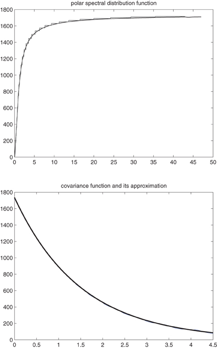
Figure 5. Above: Polar spectral distribution function and its approximation (gray). Below: True covariance function (black) and its worst approximation (gray).

The worst approximating covariance function may be calculated along the outer border of upper Figure 2, because the oscillations of the cosine-sine-Bessel surface harmonics in Equation (2) are most damped there. A look at the worst approximating covariance function in Figure 5 shows that the difference between the true covariance function and the worst approximating covariance function at the origin is 20. This is small scale variation that the approximating covariance function does not take into account. Later in spatial sampling design we will add this value of 20 to the nugget effect 106.8 of the true covariance function. Thus, 20 + 106.8 is the variance of the uncorrelated error process ϵ₀(x) in our approximating BSLM Equation (4).

We now have all quantities that we need in order to do spatial sampling design on the basis of our approximating BSLM, corresponding to the assumption of Gaussianity of observations.

7.2. Optimal Design for Gaussian Kriging

We consider to add 14 additional sampling locations from the complete design region X to the available grid of 36 sampling locations. We design for the random field of means of the original rain residuals with corresponding covariance function given in Figure 5 and being proportional to the individual covariance functions of the monthly rain residuals. Because of this proportionality, designs calculated with the mentioned covariance function would be optimal also for the individual monthly residual rainfall fields. Figure 6 shows the optimal 8 and 14 point designs. Obviously, certain locations have been selected with multiplicities larger than 1. The reason is that the Smith and Zhu design criterion does not only take account of best prediction but also of covariance estimation; in order to get the nugget effect and the behavior of the covariance function close to its origin well-estimated locations are needed in the optimal design which are close to each other. Figure 7 plots the decrease of the average of the lengths of the 95% predictive intervals when adding up to 14 design locations in an optimal way.

FIGURE 6

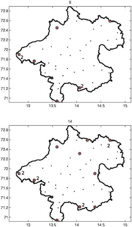
Figure 6. Above: Optimal 8 point design for Gaussian kriging. Below: Optimal 14 point design for Gaussian kriging. Certain locations have been selected with multiplicities larger than 1. Red dots: Sampling locations added.

FIGURE 7

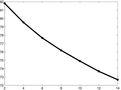
Figure 7. Average of the lengths of estimated 95% predictive intervals, when adding up to 14 design locations.

7.3. Optimal Design for Trans-Gaussian Kriging

In the above example we have assumed the data to be Gaussian and have used ordinary kriging for prediction, although, as is visible from Figure 8, the data are not Gaussian. Thus, we will consider that the standardized rainfall residuals can be transformed to Gaussianity by means of a Box-Cox transformation. Since the Box-Cox transformation works only for positive valued data we have to add a positive offset to the 12 monthly sets of standardized rainfall residuals. To identify the appropriate offset and optimal Box-Cox transformation parameter λ₀ we perform a sequence of Lilliefors tests for Gaussianity on the transformed standardized rainfall residuals. We then retain that offset and that corresponding Box-Cox transformation parameter λ₀, where the sum of the 12 p-values from the Lilliefors tests attains its maximum. Figure 9 gives the corresponding surfaces of the sum of p-values and number of rejected hypotheses for Gaussianity at the 10% significance level. According to these figures the optimal parameters are chosen as: offset = 53, λ₀ = −0.25. Obviously, for these parameters only one hypothesis of Gaussianity is rejected at the 10% significance level.

FIGURE 8

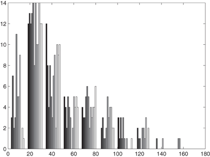
Figure 8. The 12 histograms of the rainfall residuals+53 in different shades of gray.

FIGURE 9

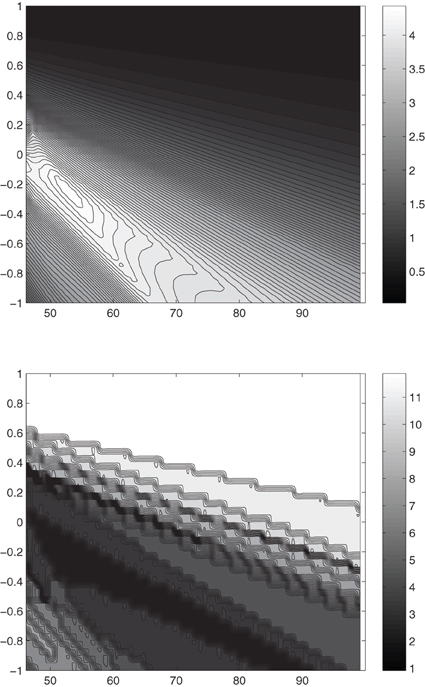
Figure 9. Above: Sum of the p-values, depending on the transformation parameter λ and the offset. Below: Number of rejected hypotheses of Gaussianity at 10% significance level, depending on the transformation parameter λ and the offset.

When designing for trans-Gaussian kriging we have the problem that the designs and the ordinary kriging predictor Ŷ_{$\widehat{\theta }$, OK}(x₀) therein are also dependent, via Equation (35), on the actual data. Since we want to find only one unique design for all 12 months, we have to agglomerate the monthly data somehow and have to design for these agglomerated data. We proceed as in the Gaussian case and consider the random field of the means of standardized rain residuals for spatial sampling design. Let R(x, i) be the original rainfall residual plus 53 at location x ∈ X and at month i = 1, 2, …, 12 and let $\widehat{\sigma }$²_i be the usual empirical estimate of the variance of the rain residuals for the i-th month. Then, standardization is performed in the following way:

$\begin{array}{ll}Z(x,i)=R(x,i)\sqrt{\frac{{\displaystyle {\sum }_{j=1}^{12}{\widehat{\sigma }}_j^2}}{12{\widehat{\sigma }}_i^2}}\hfill & (36)\hfill \end{array}$

In the following we discard that the standardization and $\widehat{\sigma }$²_i actually are estimates and assume them to be fixed and not random. According to our exploratory analysis, the random variables Z(x, i) all come from trans-Gaussian random fields with the same Gaussian covariance function and Box-Cox transformation parameter λ₀ = −0.25, but possibly different means. Consequently, Y(x, i) = g_λ0(Z(x, i)), i = 1, 2, …, 12, with g_λ0(.) denoting the Box-Cox transformation, come from Gaussian random fields with the same covariance functions but possibly different means. Assuming independence of all random fields at different months, the mean M(x) = $\frac{1}{12}{\displaystyle {\sum }_{i=1}^{12}}$ Y(x, i) also comes from a Gaussian random field with covariance function as given above, but divided by 12. As a consequence, g⁻¹_λ0(M(x)) = g⁻¹_λ0($\frac{1}{12}{\displaystyle {\sum }_{i=1}^{12}}$ g_λ0(Z(x, i))) comes from a trans-Gaussian random field with Box-Cox parameter λ₀ = −0.25 and Gaussian covariance function divided by 12. It may be shown directly that

$\begin{array}{ll}\begin{array}{l}{g}_{{\lambda }_0}^{-1}(M(x))=\\ =\frac{(\frac{1}{12}{\displaystyle {\sum }_{i=1}^{12}Z{(x,i)}^{{\lambda }_0}{)}^{1/{\lambda }_0}}}{\frac{1}{12}{\displaystyle {\sum }_{i=1}^{12}Z(x,i)}}\frac{1}{12}{\displaystyle {\sum }_{i=1}^{12}Z(x,i)}.\end{array}\hfill & (37)\hfill \end{array}$

We have validated by means of simulations that for λ₀ = −0.25 the standard deviation of the expression

$\frac{(\frac{1}{12}{\displaystyle {\sum }_{i=1}^{12}Z{(x,i)}^{{\lambda }_0}{)}^{1/{\lambda }_0}}}{\frac{1}{12}{\displaystyle {\sum }_{i=1}^{12}Z(x,i)}}$

is quite small compared to the values of $\frac{1}{12}{\displaystyle {\sum }_{i=1}^{12}}$ Z(x, i). Hence, we may assume the above expression to be constant with value d > 0, the simulated mean of above expression. Because all considered random fields are stationary, the factor d is unique to all locations x ∈ X. An alternative choice for d would be

$d=\frac{stdev(g_{{\lambda }_0}^{-1}(M(x)))}{stdev(\frac{1}{12}{\displaystyle {\sum }_{i=1}^{12}Z(x,i))}}=\frac{stdev(g_{{\lambda }_0}^{-1}(M(x)))}{\frac{1}{12}\sqrt{{\displaystyle {\sum }_{i=1}^{12}{\widehat{\sigma }}_i^2}}}$

with stdev(.) denoting standard deviation, thus making the variances to the left and right in the approximation to expression (Equation 37) equal. Thus, the distribution of $\frac{1}{12}{\displaystyle {\sum }_{i=1}^{12}}$ Z(x, i) is quite well-approximated by the distribution of $\frac{1}{d}$g⁻¹_λ0(M(x)).

It can be shown that scaling up trans-Gaussian random variables by a factor c > 0 results again in a trans-Gaussian random field, but with the corresponding Gaussian random field having as covariance function the original covariance function multiplied by c^2λ, and having as mean the original Gaussian mean multiplied by c^λ and then linearly shifted by $\frac{c^{\lambda }-1}{\lambda }$. According to this result the distribution of $\frac{1}{d}$g⁻¹_λ0(M(x)) is trans-Gaussian, too, with transformation parameter λ₀ and above mentioned unique Gaussian covariance function of the random fields {Z(x, i); x ∈ X}, i = 1, 2, …, 12 multiplied by $\frac{1}{12}$($\frac{1}{d}$)^2λ₀. The above approximation is slightly biased with respect to both, the mean and the covariance of the Gaussian random variables M(x) and the approximately Gaussian random variables g_λ0(d$\frac{1}{12}{\displaystyle {\sum }_{i=1}^{12}}$ Z(x, i)).

In our approach to spatial sampling design we can therefore assume that the random field of the means of standardized rain residuals can be approximated by a trans-Gaussian random field with Box-Cox transformation parameter λ₀ = −0.25 calculated from the 12 monthly trans-Gaussian random fields of standardized monthly rain residuals and corresponding Gaussian covariance function multiplied by $\frac{1}{12}$($\frac{1}{d}$)^2λ₀. Furthermore, we note that $\frac{1}{12}{\displaystyle {\sum }_{i=1}^{12}}$ R(x, i) = $\frac{1}{12}{\displaystyle {\sum }_{i=1}^{12}}$ Z(x, i). We thus run our optimal design algorithms from the Appendix for the agglomerated random field {$\frac{1}{12}{\displaystyle {\sum }_{i=1}^{12}}$ R(x, i); x ∈ X}, the random field of mean original raw rainfall residuals. Figure 10 shows empirical semivariogram estimates of the Box-Cox transformed standardized rain residuals and a fitted exponential semivariogram function.

FIGURE 10

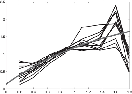
Figure 10. Empirical semivariograms of the Box-Cox transformed standardized rain residuals for all of the 12 months and a fitted exponential semivariogram (gray). The same Box-Cox parameter λ = −0.25 is used for the calculation of all variograms.

We go on to calculate the spectral distribution function corresponding to the covariance function of the Box-Cox transformed standardized rain residuals multiplied by $\frac{1}{12}$($\frac{1}{d}$)^2λ₀, its step-wise approximation and the worst approximating covariance function. We note that, close to the origin h = 0, the difference between the true covariance function and its approximation is 0.001. Finally, Figure 11 visualizes optimal 8- and 14-point designs for trans-Gaussian kriging of {$\frac{1}{12}{\displaystyle {\sum }_{i=1}^{12}}$ R(x, i); x ∈ X}. Figure 12 gives the lengths of estimated 95% predictive intervals. Obviously, the designs for trans-Gaussian kriging in Figure 11 are completely different from the designs for Gaussian kriging in Figure 6. Whereas the designs in Figure 6 are much more space-filling, the design locations in Figure 11 have been selected in areas that have high mean value of residual rainfall. This fact becomes more transparent when we compare Figures 11–13, where the predictive median of mean residual rainfall from the estimated predictive distributions of trans-Gaussian kriging is visualized. Obviously, in areas with high mean residual rainfall the average length of estimated 95% predictive intervals can be most decreased. This fact results from a fundamental difference between designs for Gaussian random fields and trans-Gaussian ones: Designs for trans-Gaussian kriging have stronger dependence on the data values themselves, through the ordinary kriging predictor in (Equation 35) and the inverse Box-Cox transformation of the corresponding estimated Gaussian predictive quantiles.

FIGURE 11

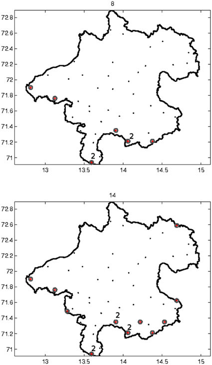
Figure 11. Above: Optimal 8 point design for trans-Gaussian kriging. Below: Optimal 14 point design for trans-Gaussian kriging. Certain locations have been selected with multiplicities larger than 1. Red dots: Sampling locations added.

FIGURE 12

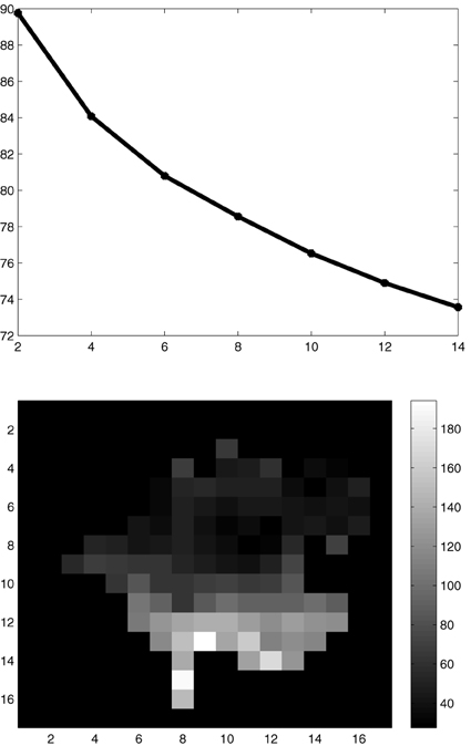
Figure 12. Above: Decrease of the average of the lengths of estimated 95% predictive intervals, when adding up to 14 design locations. Below: Lengths of estimated 95% predictive intervals corresponding to the optimal 14 point design.

FIGURE 13

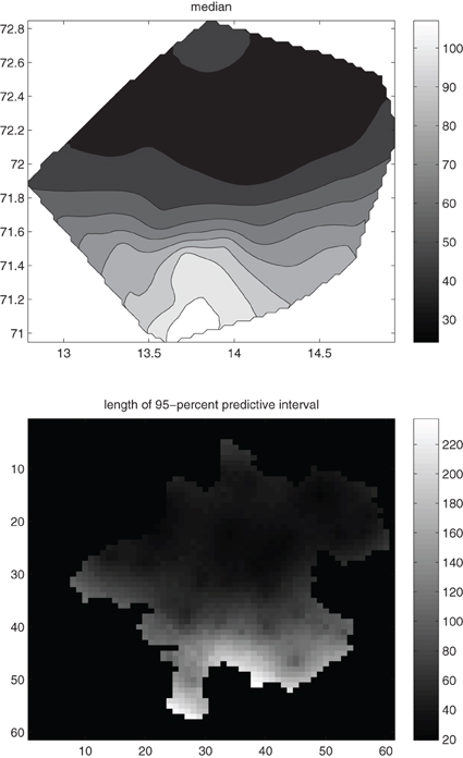
Figure 13. Above: The predictive median of the mean residual rainfall field+53 calculated from the predictive distributions of trans-Gaussian kriging applied to the 36 means of rainfall residuals+53. Below: Lengths of estimated 95% predictive intervals corresponding to the trans-Gaussian kriging from the upper figure.

Predictive maps for the original rainfall field at each month can be obtained by means of applying (trans-) Gaussian kriging also to the means of original rainfall values visible in Figure 2 and then adding these predictive maps for the mean rainfall to appropriately scaled, cp. Equation (36), predictions for the mean rainfall residuals.

According to Equation (37), we have

$\begin{array}{ll}\begin{array}{l}{g}_{{\lambda }_0}^{-1}(M(x))\approx \\ \approx d\frac{1}{12}{\displaystyle \sum _{i=1}^{12}R}(x,i)=\\ =d\frac{\frac{1}{12}{\displaystyle {\sum }_{i=1}^{12}R(x,i)}}{R(x,j)}R(x,j).\end{array}\hfill & (38)\hfill \end{array}$

By means of simulations we could once again show that for our λ₀ = −0.25 the variance of the quotient in Equation (38) is quite small. Thus, the trans-Gaussian random variables g⁻¹_λ0(M(x)), R(x, j), j = 1, 2, …, 12 and the approximately trans-Gaussian random variable $\frac{1}{12}{\displaystyle {\sum }_{i=1}^{12}}$ R(x, i) are approximately proportional to each other, with proportionality factors unique for all x ∈ X because of stationarity of the considered random fields. Moreover, we note that the above approximations are quite good because all random fields corresponding to above approximations have correct Gaussian correlation functions. Bias is introduced in the above approximations mainly in the mean of the corresponding Gaussian variables. Because the unscaled rain residuals R(x, j) are approximately proportional to $\frac{1}{12}{\displaystyle {\sum }_{i=1}^{12}}$ R(x, i) and g⁻¹_λ0(M(x)) and because the estimated predictive quantiles for random variables cZ: = c(Z(x₁), Z(x₂), …, Z(x_n))^T are c times the estimated predictive quantiles for the random variables Z: = (Z(x₁), Z(x₂), …, Z(x_n))^T, our approximately optimal designs calculated for the random variables $\frac{1}{12}{\displaystyle {\sum }_{i=1}^{12}}$ R(x, i) are approximately optimal also for the raw rain residuals R(x, j) at all months j = 1, 2, …, 12. This can be seen easily from the fact that when using the trans-Gaussian random variables cZ in Equation (35) the proportionality constant for the covariance function c^2λ₀ cancels to c^λ₀ and that the new kriging predictor is c^λ₀ times the one based on Z plus the constant $\frac{c^{{\lambda }_0}-1}{{\lambda }_0}$, observing that kriging weights sum-up to 1. Applying the inverse Box-Cox transformation to the estimated quantile given in Equation (35)

${\widehat{y}}_{1-\alpha /2,cZ}=c^{{\lambda }_0}{Y}_{OK,Z}+\frac{c^{{\lambda }_0}-1}{{\lambda }_0}+c^{{\lambda }_0}{z}_{1-\alpha /2}{\sigma }_{est,Z}$, we get

$\begin{array}{l}{({\widehat{y}}_{1-\alpha /2,cZ}{\lambda }_0+1)}^{1/{\lambda }_0}=\\ ={(c^{{\lambda }_0}(Y_{OK,Z}+z_{1-\alpha /2}{\sigma }_{est,Z}){\lambda }_0+c^{{\lambda }_0})}^{1/{\lambda }_0}\\ =c{({\widehat{y}}_{1-\alpha /2,Z}{\lambda }_0+1)}^{1/{\lambda }_0}.\end{array}$

Therefore, the 12 different design functionals are just rescaled by different proportionality factors and are otherwise approximately equivalent, with the exception that they are based on different data. Clearly, data at different times are not truly proportional, only approximately so (in distributional law). True equivalence holds if the unstandardized residuals are truly proportional to each other and to an unique trans-Gaussian variable V(x), with the same Gaussian correlation function.

One could calculate also estimated expected lengths of estimated predictive intervals by means of taking either the expectations of the ordinary kriging predictors in Equation (35), which are all unique because of stationarity, ± the expectation (or not) of the additional Gaussian-quantile times the standard deviation term, and then applying the inverse Box-Cox transformation on the expected Gaussian quantiles (Equation 35), or by means of taking expectations of the inverse Box-Cox transformed Gaussian quantiles. Then we get design criteria that are independent of the actual data values, at least with the exception that the true mean and true covariance function of the corresponding Gaussian random field must be estimated somehow. Up to date, we could not show that these two proposed approaches are equivalent, although we know that the first one is maybe more practical and mathematically easier, whereas the second one would be statistically and mathematically correct. We will follow up these approaches in a future paper. These approaches would be especially useful and necessary, when one has no data available and one desires to plan a design for a trans-Gaussian random field without having data from the scratch.

8. Discussion

8.1. Space-Time Trans-Gaussian Random Fields

A similar approach as in Section 7.3 also applies to stationary random fields Z(x, i) that are correlated in space and time and whose Gaussian correlation function can be assumed to be separable, i.e., C(Δx, Δi) = C_X(Δx) C_T(Δi), if we assume the Gaussian time-correlation function to be fixed and not estimated, and only the Gaussian spatial covariance function to be estimated by REML. As before, the trans-Gaussian R(x, i) are assumed to have the same Gaussian correlation functions, but possibly different trans-Gaussian variances $\widehat{\sigma }$²_i. Then the same standardization may be applied as above in Equation (36), and the trans-Gaussian Z(x, i) are again assumed to have the same Gaussian covariance function. The only difference to the time-uncorrelated case is that now $\frac{1}{d}$$\frac{1}{12}{\displaystyle {\sum }_{i=1}^{12}}$ R(x, i) and $\frac{1}{d}$$\frac{1}{12}{\displaystyle {\sum }_{i=1}^{12}}$ Z(x, i) do not have the same variance. We thus calculate our designs for $\frac{1}{d}$$\frac{1}{12}{\displaystyle {\sum }_{i=1}^{12}}$ Z(x, i). Let σ² be the variance of the Gaussian variables Y(x, i) = g_λ0(Z(x, i)). From the separability of the random field {Y(x, i), x ∈ X, i = 1, 2, …, 12} we conclude that the average M(x) = $\frac{1}{12}{\displaystyle {\sum }_{i=1}^{12}}$ Y(x, i) has covariance $cov(M(x_1),M(x_2))==\{\frac{1}{12}{\displaystyle {\sum }_{i,j=1}^{12}{C}_T}(|i-j|)\}\frac{{\sigma }^2}{12}{C}_X(x_1-x_2)$. This is the multiple of 1/12 times the spatial covariance function of the Y(x, i) times the constant, {$\frac{1}{12}{\displaystyle {\sum }_{i,j=1}^{12}}$ C_T(|i − j|)}. Thus, the same approach to optimal design may be applied as already discussed before. In Equation (35) the ordinary kriging predictor based on the data M(x) does not change in comparison to the uncorrelated case, because it is dependent only on the spatial correlation function, but what changes is the right-hand side of Equation (35); the original estimated standard deviation term from the time-uncorrelated case is now multiplied by $\sqrt{\frac{1}{12}{\displaystyle {\sum }_{i,j=1}^{12}{C}_T}(|i-j|)}$, due to time-correlation.

Another approach to design would be to time-decorrelate the Y(x, i) by means of multiplying for each location x ∈ X the vector [Y(x, 1), …,, Y(x, 12)] with the matrix-root of the inverse Gaussian time-correlation matrix, to average the resulting vector and to base the sampling design on these time-averages of decorrelated Gaussian standardized rain residuals. Because this time-decorrelation does not change the Gaussian spatial covariance function of the time-decorrelated Gaussian standardized residuals in comparison to the uncorrelated case, an approach similar to before results for design, with the exception that now the ordinary kriging predictor in Equation (35) is different from the original one in the uncorrelated case. However, the estimated standard deviation term in the right-hand side of Equation (35) remains the same as in the uncorrelated case, because the time-decorrelation has not changed the spatial covariance function.

It is an open question whether both proposed approaches are equivalent. We will follow-up both of the above approaches and investigate this question in one of our next papers.

Actually, in our example, trans-Gaussian kriging and optimal design could have been performed also on the original, raw data, instead of the residual rainfall data. But then, as we have found out, the Box-Cox transformation parameters for each month would not have been the same and our approach of calculating a unique design for all months would not have been possible. Instead it would have been necessary to calculate individual designs for each of the 12 months and then combine them in some way to form a single usable design.

As one reviewer proposed, the approach in this article could be generalized also to multivariate trans-Gaussian random fields. The simplest possibility would be to weight the estimated predictive lengths of the individual random fields by means of some positive weighting factors, add the weighted lengths and minimize their average over the design area. The determination of weighting factors needs some more research and will be the topic of a future paper.

8.2. Computation

Whereas the computations of the designs for the I-optimality criterion in Spöck and Pilz (2010) took only 6 h on a 3.06 Ghz CPU in MATLAB, the computations with the (Smith and Zhu, 2004) design criterion and trans-Gaussian kriging took 7 days on the same CPU and a NVIDIA GTX 580 graphics card acting as multi-coprocessor with CUDA support

http://www.nvidia.de/page/tesla/_computing/_solutions.html

The reason for this long computation time is that the averaging over the design area X must be done for the I-optimality criterion only once by means of calculating the matrix U in Equation (7) before the actual design algorithm starts. On the other hand, when using the trans-Gaussian Smith-Zhu design criterion, it is clear from the derivations in Section 6 that the averaging over the design region X must take place in every step when a new design location is tested for being added or being removed from the design.

Experimentally and theoretically it may be concluded that the computation time for trans-Gaussian Smith-Zhu design scales linearly with the number of sampling locations to be added and scales approximately with n(2M + 1) to power 75 (25 matrix multiplications), where n is the number of frequencies ω_i in the polar spectral approximation and M is the number of circular frequencies in Equation (2). In the rainfall example from Section 7 there was n = 34 and M = 45. Although we made use of the freely available GPUmat toolbox (http://gp-you.org) to parallelize matrix multiplications on the GTX 580 GPU, the computations took so much time. As we have tested, without this implementation on the GPU the computations would take 110 times longer. One disadvantage of the GPUmat toolbox is that it can work only with one single GPU but our mainboard can deal with up to 6 GPUs. In future we will investigate whether the MATLAB parallelization toolbox and JACKET (http://www.accelereyes.com) can further speed up the computations on multi-GPUs.

8.3. Conclusions and Future Developments

The preceding sections demonstrate that design functionals have a convenient and mathematically tractable structure and there is no need for stochastic search algorithms like simulated annealing in order to optimize them. The trace functional criterion is shown to be a convex functional similar to design functionals from the theory of optimal experimental design for linear regression models. Powerful tools from this theory can be used to get this criterion optimized by means of steepest descent algorithms and to show optimality of spatial sampling designs by means of equivalence theorems. The Smith and Zhu design functional, too, is shown to be continuously extendable to the compact set of continuous information matrices. To show convexity properties of this design functional remains a topic for future research. Designs with the Smith and Zhu criterion differ from designs with the trace functional: Because the Smith and Zhu design criterion takes the uncertainty and estimation of the covariance function into account, resulting designs with this criterion must have sampling locations very close to each other as well as space-filling locations. Designs resulting from optimization of the trace functional only show quite regular space filling locations. Designs for trans-Gaussian kriging on the other hand via minimizing the average of the lengths of estimated predictive intervals also are strongly dependent on the data values themselves, in sharp contrast to designs for Gaussian kriging without REML correction, which, if the covariance function can be assumed to be certain, are completely independent of the data. Furthermore, we remark that a similar approach for spatial sampling design of non-stationary random fields is under development (cp. also Spöck and Pilz, 2008) and will soon become freely available in the spatDesign toolbox of the first author, see (Spöck, 2011). Because this toolbox is freely available, researchers may use it for their own problems in spatial sampling design. It is easy to use, demonstrations are included as in Spöck (2012). Really useful is the toolbox mainly for data that have, like in our data example skew marginal distributions so that the advantages of trans-Gaussian kriging and sampling design come to bear. Such skew data may be found all over our environment: Rainfall, radioactivity, air-, surface-, and groundwater pollutants are only some examples. Similar methods for “spatial” sampling design may be used also in the response surface design of computer simulation experiments, where “spatial” coordinates correspond here to the values of certain parameters at which the computer simulations should be run.

Currently we work on an extension of the trans-Gaussian sampling design approach to stochastic partial differential equations guiding, for example, the dispersion of pollutants in space and time. This approach will consider also mobile sensors.

The main reason that lead us to the polar spectral approximation is that by means of this approximation we are actually in the context of Bayesian regression models whose additional linearity makes many things much easier.

Conflict of Interest Statement

The authors declare that the research was conducted in the absence of any commercial or financial relationships that could be construed as a potential conflict of interest.

References

Abt, M. (1999). Estimating the prediction mean squared error in Gaussian stochastic processes with exponential correlation structure. Scand. J. Stat. 26, 563–578.

Google Scholar

Aarts, E. H., and Korst, J. (1989). Simulated Annealing and Boltzman Machines. New York, NY: Wiley.

Baume, O. P., Gebhardt, A., Gebhardt, C., Heuvelink, G. B. M., and Pilz, J. (2011). Network optimization algorithms and scenarios in the context of automatic mapping. Comput. Geosci. 37, 289–294. doi: 10.1016/j.cageo.2010.04.014

CrossRef Full Text | Google Scholar

Brown, P. J., Le, N. D., and Zidek, J. V. (1994). Multivariate spatial interpolation and exposure to air pollutants. Can. J. Stat. 2, 489–509.

Google Scholar

Brus, D. J., and de Gruijter, J. J. (1997). Random sampling or geostatistical modeling? Choosing between design-based and model-based sampling strategies for soil (with discussion). Geoderma 80, 1–44.

Google Scholar

Brus, D. J., and Heuvelink, G. B. M. (2007). Optimization of sample patterns for universal kriging of environmental variables. Geoderma 138, 86–95. doi: 10.1016/j.geoderma.2006.10.016

CrossRef Full Text | Google Scholar

Chen, V. C. P., Tsui, K. L., Barton, R. R., and Meckesheimer, M. (2006). A review on design, modeling and applications of computer experiments. IIE Trans. 38, 273–291. doi: 10.1080/07408170500232495

CrossRef Full Text | Google Scholar

Diggle, P., and Lophaven, S. (2006). Bayesian Geostatistical Design. Scand. J. Stat. 33, 53–64. doi: 10.1111/j.1467-9469.2005.00469.x

CrossRef Full Text | Google Scholar

Fedorov, V. V. (1972). “Theory of optimal experiments,” in Russian Original: Nauka, Moscow 1971, transl. and eds W. J. Studden and E. M. Klimko (New York, NY: Academic Press), 306.

Fedorov, V. (1996). “Design of spatial experiments: model fitting and prediction,” in Handbook of Statistics, Vol. 13, eds S. Ghosh and C. R. Rao (Amsterdam: Elsevier), 515–553.

Fedorov, V. V., and Flanagan, D. (1997). Optimal monitoring network design based on Mercer's expansion of the covariance kernel. J. Combinat. Inf. Syst. Sci. 23, 237–250.

Fuentes, M., Chaudhuri, A., and Holland, D. M. (2007). Bayesian entropy for spatial sampling design of environmental data. J. Environ. Ecol. Stat. 14, 323–340. doi: 10.1007/s10651-007-0017-0

CrossRef Full Text | Google Scholar

Gebhardt, C. (2003). Bayesian Methods for Geostatistical Design. Ph.D. Thesis, University of Klagenfurt, Austria.

Gramacy, R. B., and Lee, H. K. H. (2008). Bayesian treed Gaussian process models with an application to computer modeling. J. Am. Stat. Ass. 103, 1119–1130. doi: 10.1198/016214508000000689

CrossRef Full Text | Google Scholar

Gramacy, R. B., and Lee, H. K. H. (2011). “Optimization under unknown constraints,” in Bayesian Statistics 9, ed. J. M. Bernardo, M. J. Bayarri, J. O. Berger, A. P. Dawid, D. Heckerman, A. F. M. Smith, and M. West (New York, NY: Oxford University Press), 19.

Groenigen, J. W., van Siderius, W., and Stein, A. (1999). Constrained optimisation of soil sampling for minimisation of the kriging variance. Geoderma 87, 239–259.

Google Scholar

Harville, D. A., and Jeske, D. R. (1992). Mean squared error of estimation or prediction under a general linear model. J. Am. Stat. Assoc. 87, 724–731.

Google Scholar

Hu, M. G., and Wang, J. F. (2011). A spatial sampling optimization package using MSN theory. Environ. Model. Softw. 26, 546–548. doi: 10.1016/j.envsoft.2010.10.006

CrossRef Full Text | Google Scholar

Kiefer, J. (1959). Optimum experimental design. J. R. Stat. Soc. Ser. B Stat. Soc. 21, 272–319.

PubMed Abstract | Google Scholar

Kleijnen, J. P. C., and van Beers, W. C. M. (2004). Application driven sequential design for simulation experiments: kriging metamodeling. J. Oper. Res. Soc. 55, 876–893. doi: 10.1057/palgrave.jors.2601747

CrossRef Full Text | Google Scholar

Le, N. D., and Zidek, J. V. (2009). Statistical Analysis of Environmental Space-Time Processes. New York, NY: Springer.

Google Scholar

Li, J., and Bardossy, A. (2011). A Copula based observation network design approach. Environ. Model. Softw. 26, 1349–1357. doi: 10.1016/j.envsoft.2011.05.001

CrossRef Full Text | Google Scholar

Lim, Y. B., Sacks, J., and Studden, W. J. (2002). Design and analysis of computer experiments when the output is highly correlated over the input space. Can. J. Stat. 30, 109–126. doi: 10.2307/3315868

CrossRef Full Text | Google Scholar

Mateu, J., and Müller, W. G. (2012). Spatio-Temporal Design: Advances in Efficient Data Acquisition. New York, NY: Wiley.

Google Scholar

Mitchell, T. J., and Morris, M. D. (1992). Bayesian design and analysis of computer experiments: two examples. Stat. Sin. 2, 359–379.

Google Scholar

Morris, M. D., Mitchell, T. J., and Ylvisaker, D. (1993). Bayesian design and analysis of computer experiments: use of derivatives in surface prediction. Technometrics 35, 243–255.

Google Scholar

Müller, P., Sanso, B., and De Iorio, M. (2004). Optimal bayesian design by inhomogeneous Markov chain simulation. J. Am. Stat. Assoc. 99, 788–798. doi: 10.1198/016214504000001123

CrossRef Full Text | Google Scholar

Müller, W. G., and Pazman, A. (1998). Design measures and approximate information matrices for experiments without replications. J. Stat. Plann. Inference 71, 349–362.

Google Scholar

Müller, W. G., and Pazman, A. (1999). An algorithm for the computation of optimum designs under a given covariance structure. J. Comput. Stat. 14, 197–211.

Google Scholar

Müller, W. G., Pronzato, L., Rendas, J., and Waldl, H. (2015). Efficient prediction designs for random fields. Appl. Stochast. Models Bus. Ind 31, 178–194. doi: 10.1002/asmb.2084

CrossRef Full Text | Google Scholar

Müller, W. G. (2005). A comparison of spatial design methods for correlated observations. Environmetrics 16, 495–505. doi: 10.1002/env.717

CrossRef Full Text | Google Scholar

Müller, W. G., and Zimmerman, D. L. (1999). Optimal designs for variogram estimation. Environmetrics 10, 23–37.

Google Scholar

Omre, H., and Halvorsen, K. (1989). The Bayesian bridge between simple and universal kriging. Math. Geol. 21, 767–786.

Google Scholar

Pazman, A., and Müller, W. G. (2001). Optimal design of experiments subject to correlated errors. Stat. Probab. Lett. 52, 29–34. doi: 10.1016/S0167-7152(00)00201-7

PubMed Abstract | CrossRef Full Text | Google Scholar

Pilz, J. (1991). Bayesian Estimation and Experimental Design in Linear Regression Models. New York, NY: Wiley.

Schonlau, M. (1997). Computer Experiments and Global Optimization. Ph.D. dissertation, University of Waterloo, Canada.

Smith, R. L., and Zhu, Z. (2004). Asymptotic Theory for Kriging with Estimated Parameters and its Application to Network Design. Technical Report, University of North Carolina.

Spöck, G., and Pilz, J. (2010). Spatial sampling design and covariance-robust minimax prediction based on convex design ideas. Stochast. Environ. Res. Risk Assess. 24, 463–482. doi: 10.1007/s00477-009-0334-y

CrossRef Full Text | Google Scholar

Spöck, G., and Pilz, J. (2008). “Non-stationary spatial modeling using harmonic analysis,” in Proceedings of the Eight International Geostatistics Congress, eds J. M. Ortiz and X. Emery (Santiago: Gecamin), 389–398.

Spöck, G. (2011). spatDesign V.2.1.0: Matlab/Octave Spatial Sampling Design Toolbox. Available online at: http://wwwu.uni-klu.ac.at/guspoeck/spatDesignMatlab.zip; http://wwwu.uni-klu.ac.at/guspoeck/spatDesignOctave.zip

Spöck, G. (2012). Spatial sampling design based on spectral approximations to the random field Environ. Model. Softw. 33, 48–60. doi: 10.1016/j.envsoft.2012.01.004

CrossRef Full Text | Google Scholar

Whittle, P. (1973). Some general points in the theory and construction of D-optimum experimental designs. J. R. Stat. Soc. Ser. B Stat. Soc. 35, 123–130.

Trujillo-Ventura, A., and Ellis, J. H. (1991). Multiobjective air pollution monitoring network design. Atmos. Environ. 25, 469–479.

Google Scholar

Yaglom, A. M. (1987). Correlation Theory of Stationary and Related Random Functions. New York, NY: Springer-Verlag.

Zhu, Z., and Stein, M. L. (2006). Spatial sampling design for prediction with estimated parameters. J. Agric. Biol. Environ. Stat. 11, 24–44. doi: 10.1198/108571106X99751

CrossRef Full Text | Google Scholar

Zimmerman, D. L., and Lie, J. (2013). “Model-based frequentist design for univariate and multivariate geostatistics,” in Spatio-Temporal Design: Advances in Efficient Data Acquisition, eds J. Mateu and W. Müller (Chichester, UK: Wiley), 37–53.

Zimmerman, D. L. (2006). Optimal network design for spatial prediction, covariance parameter estimation, and empirical prediction. Environmetrics 17, 635–652. doi: 10.1002/env.769

CrossRef Full Text | Google Scholar

A1. Appendix

A1.1. Iteration Procedures for Determining Exact Designs

We are now going to formulate iteration procedures for the construction of approximately optimal exact designs. Contrary to the construction of optimal discrete designs, here we cannot prove convergence of the exact designs to the functional value Ψ(d*) of an optimal exact design d*; we can only guarantee stepwise improvement of a given exact starting design, i.e., the sequence of functional values Ψ(d_{n, s}) decreases monotonically with increasing iteration index s. The algorithm is an exchange algorithm improving n-point designs and starts with a given initial design.

A1.1.1. Exchange algorithm:

Step 1. Use some initial design d_{n, 1} = {x_{1, 1}, …, x_{n, 1}} ∈ Xⁿ of size n.

Step 2. Beginning with s = 1, form the design d_{n+1, s} = d_{n, s} + (x_{n+1, s}) by adding the point

$x_{n+1,s}=\text{arg}\underset{x\in X}{\min }\Psi (M_B(d_{n,s}+(x)))$

to d_{n, s}.

Then form d^j_{n, s} = d_{n+1, s} − (x_{j, s}), j = 1, 2, …, n + 1 and delete that point x_j*, _s from d_{n+1, s} for which

$\Psi (M_B(d_{n,s}^{j^{*}}))=\underset{{}_{j\in \{1,\dots ,n+1\}}}{\min }\Psi (M_B(d_{n,s}^j))).$

Step 3. Repeat Step 2 until the point to be deleted is equivalent to the point to be added.

For the design functional (Equation 8), Step 2 is determined as follows:

x_{n + 1, s} maximizes (over X)

$\frac{h{(x)}^T{M}_B{(d_{n,s})}^{-1}U{M}_B{(d_{n,s})}^{-1}h(x)}{n+h{(x)}^T{M}_B{(d_{n,s})}^{-1}h(x)}.$

j* is the index which minimizes

$\frac{h{(x_{j,s})}^T{Q}_B(d_{n+1,s})h(x_{j,s})}{n+1-h{(x_{j,s})}^T{M}_B{(d_{n+1,s})}^{-1}h(x_{j,s})},$

where

$Q_B(d_{n+1,s})=M_B{(d_{n+1,s})}^{-1}U{M}_B{(d_{n+1,s})}^{-1}.$

For the Smith and Zhu design criterion no such simplification exists and the complete design functional (Equations 9, 35) must be recalculated in every step.

A1.1.2. Generation of an initial design

The starting design is taken as a one-point design which minimizes the design functional among all designs of size n = 1. Note that such a design exists since the Bayesian information matrix is positive definite even for designs of size n = 1.

Step 1. Choose x₁ ∈ X such that

x₁ = arg min_x∈XΨ(M_B((x))), and set d₁ = (x₁).

Step 2. Beginning with i = 1, find x_i+1 such that x_i+1 = arg min_x∈XΨ(M_B(d_i + (x))) and form d_i+1 = d_i + (x_i+1). Continue with i replaced by i + 1 until i + 1 = n.

Step 3. If i + 1 = n then stop and take

d_{n, 1} = {x₁, …, x_n} as an initial design.

It is a good idea to combine the initial design algorithm Section A1.1.2 and the exchange algorithm Section A1.1.1.

A1.1.3. Reduction of experimental designs

Often it is desired to reduce a given experimental design d = {x₁, x₂, …, x_n} to one including only m < n design points from d:

Step 1. Delete that design point x_j* from d for which

x_j* = arg min_xj∈vΨ(M_B(d − (x_j))), and set

d: = d − (x_j⁻).

Step 2. Iterate Step 1 until the design d contains only m design points.

Also, this algorithm may be combined with an improvement step similar to the exchange algorithm Section A1.1.1. In algorithm Section A1.1.1 the calculation of x_{n + 1, s} has merely to be replaced by

$x_{n+1,s}=\text{arg}\underset{x\in d-d_{n,s}}{\min }\Psi (M_B(d_{n,s}+(x))),$

where d is the initial design that has to be reduced. This improved algorithm has the advantage that design points, once deleted, can reenter the design in the exchange step.

A1.1.4. Determining the inverse of the information matrix

Obviously, the calculation of exact designs requires in every step the calculation of the inverses of the information matrices M_B(d_{n, s}) and M_B(d_{n + 1, s}). We saw that these information matrices can have a quite high dimension of about 4000 × 4000. So, how can one invert such large matrices in affordable time? A first artificial, inverse information matrix in spatial sampling design can always be one with block-diagonal structure corresponding to 0 selected design points, having one very small block, being the a priori covariance matrix for deterministic trend functions, and having one further block, being just a diagonal matrix of very high dimension (about 4000 diagonal elements, being the variances of the stochastic amplitudes resulting from a harmonic decomposition of the random field into sine-cosine-Bessel surface harmonics). So, no inversion is needed at a first step. The inversion of all other information matrices becomes easy, and there is computationally no need to make explicit use of numerical matrix inversion algorithms, when one considers Equations (13.26, 13.28) in Pilz (1991):

$\begin{array}{l}{M}_B{(d_{n,s}+(x))}^{-1}=\frac{n+1}{n}\{M_B{(d_{n,s})}^{-1}\\ -\frac{M_B{(d_{n,s})}^{-1}h(x)h{(x)}^T{M}_B{(d_{n,s})}^{-1}}{n+h{(x)}^T{M}_B{(d_{n,s})}^{-1}h(x)}\},\\ M_B{(d_{n,s}^j)}^{-1}=\frac{n}{n+1}\{M_B{(d_{n+1,s})}^{-1}\\ +\frac{M_B{(d_{n+1,s})}^{-1}h(x_{j,s})h{(x_{j,s})}^T{M}_B{(d_{n+1,s})}^{-1}}{n+1-h{(x_{j,s})}^T{M}_B{(d_{n+1,s})}^{-1}h(x_{j,s})}\}\end{array}$

Obviously, only matrix- and vector multiplications are needed in these update formulae.