Graph neural network-based water contamination detection from community housing information

Introduction: Detecting water contamination in community housing is crucial for protecting public health. Early detection enables timely action to prevent waterborne diseases and ensures equitable access to safe drinking water. Traditional methods recommended by the Environmental Protection Agency (EPA) rely on collecting water samples and conducting lab tests, which can be both time-consuming and costly.

Methods: To address these limitations, this study introduces a Graph Attention Network (GAT) to predict lead contamination in drinking water. The GAT model leverages publicly available municipal records and housing information to model interactions between homes and identify contamination patterns. Each house is represented as a node, and relationships between nodes are analyzed to provide a clearer understanding of contamination risks within the community.

Results: Using data from Flint, Michigan, the model demonstrated higher performance compared to traditional methods. Specifically, the GAT achieved an accuracy of 0.80, precision of 0.71, and recall of 0.93, outperforming XGBoost, a classical machine learning algorithm, which had an accuracy of 0.70, precision of 0.66, and recall of 0.67.

Discussion: In addition to its predictive capabilities, the GAT model identifies key factors contributing to lead contamination, enabling more precise targeting of at-risk areas. This approach offers a practical tool for policymakers and public health officials to assess and mitigate contamination risks, ultimately improving community health and safety.

1 Introduction

Detecting contamination in drinking water is critical for safeguarding public health, as it prevents exposure to harmful pollutants and ensures access to safe drinking water. In the United States, nearly one-fifth of the population, approximately 63 million people, have been exposed to potentially unsafe water multiple times over the past decade (News21, 2023). An investigation by the Environmental Protection Agency (EPA) reported over 680,000 water quality violations, affecting communities ranging from rural Central California to urban New York City. This widespread issue underscores the need for effective detection methods that address both the severity and scale of contamination. Health risks associated with lead in drinking water are well-documented, with even minimal concentrations posing significant concerns. Although the EPA has established an action level of 15 ppb for lead (Pb), no concentration is considered entirely safe because lead is non-biodegradable and can accumulate in the food chain (Doré et al., 2020; Han et al., 2020; Sawan et al., 2020). Prolonged exposure can harm the brain, kidneys, and other organs (Vlachou et al., 2020; Martin and Griswold, 2009; Trueman et al., 2016).

Lead service lines (LSLs) are a primary source of contamination, contributing 50%–75% of the lead mass in drinking water, followed by premise piping (20%–35%) and faucets (1%–3%) (Sandvig et al., 2008). In the U.S., an estimated 6.1 to 10.2 million LSLs supply water to approximately 15–22 million people, accounting for about 7% of community water system consumers (Cornwell et al., 2016; Hensley et al., 2021). Addressing LSLs is critical for reducing lead exposure risks and safeguarding public health.

Various methods exist for detecting LSLs, including record screening, visual inspections, water quality testing (e.g., EPA methods 200.8 and 200.9), excavation, and advanced techniques like cumulative lead sampling devices and acoustic wave technology (Hensley et al., 2021). More recently, predictive data analysis, particularly machine learning, has emerged as a cost-effective alternative. Machine learning enables researchers to analyze patterns in existing data, identifying high-risk areas without relying on expensive sampling or specialized equipment. By focusing on areas most at risk, these models support more efficient mitigation efforts and help reduce lead exposure in drinking water.

The extent of lead release from LSLs depends on a combination of factors, including water chemistry, pipe scale composition, and environmental conditions (Pasteris et al., 2021; García-Timermans et al., 2023). Tools such as Raman spectroscopy have been used to analyze the stability of lead-pipe scales under changing treatment conditions, providing insights into how factors like pH adjustments, disinfectants, and orthophosphate dosing affect lead release (Pasteris et al., 2021). Similarly, pilot-scale water distribution studies have shown that biofilm formation, pipe aging, and transport conditions also influence water quality (García-Timermans et al., 2023). To mitigate these factors and manage lead release, effective corrosion control strategies are essential.

Corrosion control strategies play an important role in managing lead release from service lines. Zinc orthophosphate has been effective in reducing nitrate-induced lead corrosion, particularly in systems with high nitrate levels (Lopez et al., 2024). However, challenges such as aluminum accumulation in pipe scales can delay the performance of phosphate inhibitors, indicating the need for adaptive strategies (Li et al., 2020). The composition of pipe scales influences lead dynamics: iron-rich scales accelerate the oxidation of Pb(II) to Bae et al. (2020b), while manganese facilitates the oxidation of lead carbonate, stabilizing PbO formation in chlorinated systems (Pan et al., 2019). Interactions with other metals, such as chromium, add further complexity. Chromium release from pipe scales is influenced by anion concentrations; sulfate and chloride promote release under certain conditions (Devine et al., 2024; Ni et al., 2024; Bae et al., 2020a). Orthophosphate can stabilize lead release by forming calcium–lead–phosphorus solids, but trade-offs like calcium phosphate precipitation illustrate the complexities of balancing corrosion control and water quality (Bae et al., 2020c; Devine et al., 2024). These findings highlight the intricate interplay among water chemistry, pipe materials, and environmental factors in determining lead behavior in drinking water systems. Understanding these dynamics emphasizes the need for predictive tools to effectively address lead contamination.

Machine learning offers an approach to complement traditional water quality assessments by modeling interactions between water chemistry, pipe scales, and environmental factors. These models provide insights that help identify areas of elevated contamination risk and guide targeted mitigation strategies. Unlike traditional methods that often require extensive infrastructure interventions, machine learning leverages spatial and temporal data to improve the accuracy of risk predictions. This approach addresses challenges such as variable lead levels and incomplete service line data, enabling more efficient resource allocation and decision-making.

Recent studies have applied machine learning models to address lead contamination. Random Forest models achieved cross-validation scores of 0.88 for Massachusetts and 0.78 for California (Lobo et al., 2022). In Pittsburgh, precise predictions (over 90%) were made for only 13% of customers, suggesting that unnecessary excavations could be reduced by improving short-term replacement decisions (Hajiseyedjavadi et al., 2022). Incorporating field observations of tap water materials further improved prediction accuracy to 94% when integrated into models (Blackhurst, 2021). Gradient Boosting models predicted high lead levels (over 15 ppb) in tap water for the Pittsburgh Water and Sewer Authority, achieving an AUC score of 71.6% (Hajiseyedjavadi et al., 2022). Similarly, Support Vector Machines identified lead service lines with an average accuracy of 90% (Gurewitsch, 2019). In Flint, Michigan, an XGBoost model identified 1,000 homes most likely to exceed the EPA’s action level of 15 ppb, even without direct test results (Chojnacki et al., 2017).

Despite these advancements, challenges remain. Imbalanced datasets can bias model training, and incomplete or inaccurate service line data compromise prediction reliability. The variability of lead levels adds complexity, and many models focus exclusively on lead results without incorporating spatial factors such as proximity to contamination sources. Addressing these limitations is crucial for improving the accuracy and broader applicability of machine learning models.

Machine learning applications for lead contamination have been explored across diverse regions. In Flint, Michigan, researchers developed predictive models combining residential water test data with infrastructure information, though these efforts faced computational and data limitations (Abernethy et al., 2016). In Saudi Arabia, techniques like Nonlinear Autoregressive Neural Networks and Long Short-Term Memory networks were used to predict the Water Quality Index, but the findings were specific to that region (Aldhyani et al., 2020). In Chicago, Illinois, models such as Random Forest, logistic regression, and support vector machines assessed lead poisoning risks in children, often focusing on lead paint rather than waterborne contamination (Potash et al., 2015). In Pittsburgh, Pennsylvania, Support Vector Machine and Random Forest models assessed lead service line risks in residential areas, but their performance was limited by incomplete data and a narrow focus on factors like housing age and spatial characteristics (Hajiseyedjavadi et al., 2020; Gurewitsch, 2019). Similarly, in California and Massachusetts, Random Forest models identified high-risk areas for lead in school drinking water, relying heavily on publicly available data without establishing causality (Lobo et al., 2022).

Given the complexity of environmental data and the limitations of existing models, advanced methods are required to address these challenges. This study applies GATs to lead contamination risk assessment, leveraging their ability to capture geographic relationships and complex interactions. Previous research on Graph Neural Networks (GNN) has shown their effectiveness in environmental and water management tasks. For example, Graph Convolutional Recurrent Neural Networks (GCRNN) have been applied to water demand forecasting, capturing spatial and temporal dependencies (Zanfei et al., 2022). Similarly, GNN have been used in groundwater level prediction in British Columbia, Canada, by representing wells as graph nodes and learning spatial relationships through a self-adaptive adjacency matrix (Bai and Tahmasebi, 2023). In river networks, GATs combined with spatiotemporal fusion have modeled spatial dependencies among nodes and temporal dynamics (Lin et al., 2022). These applications suggest that GATs have the potential to improve predictions of lead contamination in drinking water.

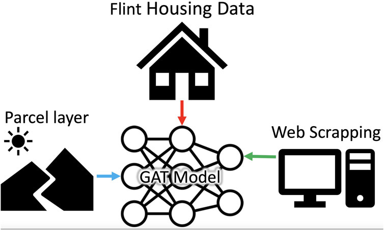
While lead service lines remain a primary source of contamination, this study focuses on developing predictive tools to assess contamination risks rather than conducting direct experimentation on service lines. By utilizing GATs, this research aims to address the limitations of existing machine learning models and enhance risk assessment accuracy. The study contributes to the field by providing a robust framework for contamination prediction, integrating spatial dependencies and environmental factors. To provide a structured view of the implemented approach, Figure 1 summarizes the key steps involved in the water contamination detection framework.

Figure 1

Figure 1. Gnn development with multiple data sources.

2 Materials and methods

2.1 Data collection

Our study is centered on the city of Flint, Michigan, which has been facing a significant crisis due to lead contamination in its water supply (Michigan.gov, 2023). Our initial dataset was derived from the water testing services in Flint, in collaboration with the Michigan Department of Environmental Quality (Michigan.gov, 2023). This dataset spans January through December 2016, capturing household-level water sampling efforts undertaken after the Flint water crisis. The time frame is critical, as it reflects lead contamination trends during early remediation measures, including the introduction of corrosion control. This dataset comprised approximately 14,000 records, predominantly from the year 2016 as mentioned earlier. However, the limited diversity of features within this dataset rendered it inadequate for machine learning analysis.

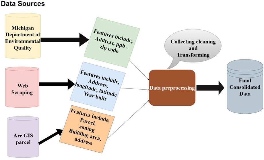
To address this limitation, we utilized web scraping techniques to augment our dataset with additional property information from the Zillow online real estate database (www.zillow.com) (Sarr and Diallo, 2018; Zillow, 2023). The web scraping process was implemented using Python, which provided flexibility for data retrieval and processing. The approach used libraries like googlesearch-python to programmatically retrieve URLs via Google searches, requests and json for HTTP requests and API responses, and pandas for handling and storing the data. Additional utilities, such as io and time, supported auxiliary tasks. The scraping process began by identifying relevant links using googlesearch-python, followed by parsing HTML content and integrating with RapidAPI to extract structured data about properties. Key attributes, such as longitude and latitude, building size, year built, and condition, were systematically stored in Comma-Separated Values (CSV) format for downstream analysis. To ensure the validity and accuracy of the web-scraped data, we cross-referenced residential addresses and features (e.g., year built) with the Michigan Department of Environmental dataset and Arc GIS parcel records. This validation step confirmed the consistency of the scraped data and ensured its reliability for further analysis. The web scraping process retrieved approximately 1,070 property records. Following the cleaning and validation steps described, 154 records were excluded due to missing over 80% of key features, such as longitude and latitude, building size, year built, and condition or due to a lack of alignment with other sources. This left 916 records that met the inclusion criteria. These excluded records were largely incomplete and unlikely to impact the findings or the model’s ability to generalize contamination patterns. This cleaning and validation process was applied uniformly across the dataset to maintain integrity and avoid systematic bias. Figure 2 illustrates our entire data source.

Figure 2

Figure 2. Workflow for data consolidation from multiple sources for lead contamination analysis.

Furthermore, we enriched our dataset with Arc GIS parcel record data from the City of Flint office, incorporating critical property details such as location and valuation to enhance the depth of our analysis. Any inconsistencies or unmatched data were omitted to maintain data integrity. Additionally, we examined seasonal variations in lead concentrations to determine whether temperature fluctuations or changes in water usage patterns influenced contamination levels. A seasonal breakdown of lead levels showed minor variations, with slightly higher concentrations in summer and fall and lower levels in winter. These trends suggest that increased corrosion in warmer months and shifts in water demand may have contributed to fluctuations. However, the differences were not large enough to indicate strong seasonal dependence.

2.2 Geographic information system mapping in flint

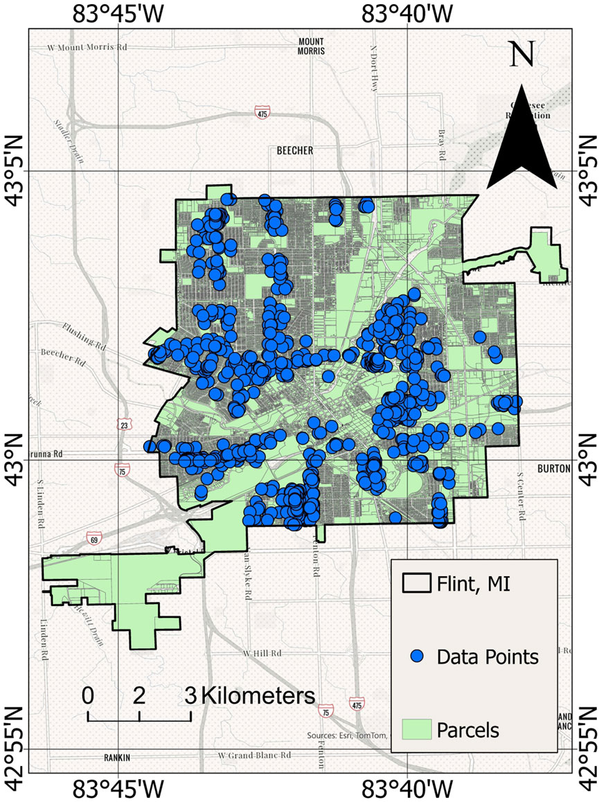
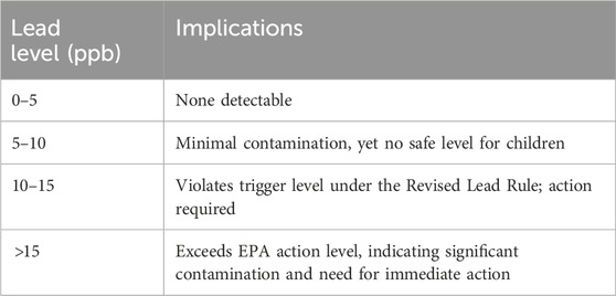
To provide a visual representation of our study area, Figure 3 presents a GIS map indicating the houses in Flint that were sampled for these prediction studies. Such a map offers a spatial understanding of the scope of our research and the distribution of samples across the city. The data for our study was carefully sampled homes from the initial dataset of 14,000 records. Homes with higher lead concentrations were prioritized to train the model effectively in identifying contamination patterns. This approach ensured that the dataset was representative of homes across various lead contamination levels, as categorized in Table 1.

Figure 3

Figure 3. GIS map showing sampled houses in Flint for prediction studies.

Table 1

Table 1. Lead contamination range (ppb) and categorization.

2.3 Data curation

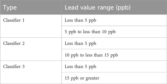
To focus on houses affected by varying lead levels, we adopted a labeling scheme aligned with EPA standards (Agency, 2023). Houses with lead levels below 5 ppb were categorized as Level 0; those with levels from five to less than 10 ppb as Level 1; from 10 to less than 15 ppb as Level 2; and houses with lead levels of 15 ppb or higher as Level 3 Table 2. These classification thresholds reflect real-world standards, enabling the model to detect and differentiate multiple levels of lead contamination severity. Recognizing that no level of lead is entirely safe, this scheme emphasizes early detection and intervention. By identifying contamination even at minimal levels, the model aims to provide actionable insights to mitigate risks and facilitate timely responses.

Table 2

Table 2. Lead contamination range and implications.

Out of the initial 14,000 records, only 916 homes met the inclusion criteria for our analysis. Specifically, each included home had consistent and verified data across all sources (Michigan Department of Environmental dataset, Zillow, and Arc GIS records). Samples that lacked corresponding information or exhibited more than 80% missing data were excluded. This stringent cleaning process ensured a quality dataset for modeling. Each lead sample was also matched to a specific parcel of land in Flint, and one-hot encoding and normalization techniques were applied to the final dataset, following best practices outlined in Kuhn and Johnson (2013).

Each dataset was categorized based on lead contamination levels according to the EPA standards Table 2. The lead levels are divided into four categories:

Proportions and Counts.

• Level 0: 59.5% of the homes (545 homes) are categorized as Level 0, indicating minimal lead contamination. Lead levels less than 5 ppb

• Level 0: 59.5% of the homes (545 homes) are categorized as Level 0, indicating minimal lead ad levels between 5 and 10 ppb

• Level 0: 59.5% of the homes (545 homes) are categorized as Level 0, indicating minimal lead Level 2: 8.2% of the homes (75 homes) are in Level 2, with moderate lead contamination. Lead levels between 10 and 15 ppb

• Level 0: 59.5% of the homes (545 homes) are categorized as Level 0, indicating minimal lead Level 3: 15.6% of the homes (143 homes) are classified as Level 3, showing the highest levels of lead contamination. Lead levels 15 ppb or greater

The dataset is predominantly composed of homes with very low or no lead contamination (Level 0). However, a significant portion of the dataset (approximately 40.5%) consists of homes with varying degrees of lead contamination (Levels 1, 2, and 3). This stratification was crucial for ensuring the model could learn to identify both contaminated and homes at very low risk of contamination effectively. While minor seasonal variations in lead levels were observed, they do not significantly impact the overall assessment of contamination risk. The seasonal trends suggest that lead levels remain relatively stable throughout the year, with slight increases in warmer months. This reinforces the importance of long-term monitoring beyond seasonal patterns, as lead contamination is influenced by multiple factors beyond temperature fluctuations. Although this dataset does not represent the entire population of Flint homes, it provides a robust sample for testing and refining the model. The inclusion criteria ensured data quality and reliability, while the prioritization of contaminated homes allowed the model to focus on identifying risk patterns. This study lays the foundation for future work with larger, more representative datasets.

In summary, we utilize data from Flint, Michigan’s lead contamination crisis to develop a machine-learning model for the detection of lead in drinking water.

2.4 Machine learning models

We employed GAT for our primary model, developed using libraries including PyTorch, PyTorch Geometric, NetworkX, and GeoPy (Veličković et al., 2018). For ensemble modeling, we used classical machine learning algorithms such as RandomForestClassifier, SVC, and XGBoost (Abernethy et al., 2016). The models’ performance was assessed using metrics like the Receiver Operating Characteristic (ROC) curve, ROC, and the AUC score. Throughout this process, we adhered to ethical guidelines, particularly ensuring that data was not publicly accessible online, to safeguard our dataset’s privacy and ethical integrity (Floridi and Taddeo, 2016).

2.5 Graph attention network

The Graph Attention Network (GAT), a specialized variant of Graph Neural Networks (GNNs), incorporates an attention mechanism to emphasize the influence of specific neighboring nodes. This approach was introduced in the study by Veličković et al. (2018). The attention mechanism, originally developed for sequence-based tasks, has been applied in areas such as machine translation (Bahdanau and Bengio, 2015; Vaswani et al., 2017). More recently, this concept has been adapted for graph-based applications, resulting in various models that integrate the attention operator into graph neural networks. The work by Veličković et al. (2018) represents an important step in extending attention-based methods to graph-structured data.

In this study, we utilize the GAT model to generate higher-level feature representations. The model applies self-attention mechanisms to an input graph composed of $N$ nodes, each with $F$. Our implementation diverges from the original architecture by employing a single attention head, simplifying computations without significantly compromising performance (Veličković et al., 2018). The input to the GAT layer is a set of node features, represented as shown in Equations 1–4:

$h=\left\{{\vec{h}}_1,{\vec{h}}_1,\dots ,{\vec{h}}_N,\right\}(1)$

Here ${\vec{h}}_i\in {\mathbb{R}}^F$. The layer produces a new set of node features, potentially with different cardinality ${\mathbf{F}}^{\prime }$, denoted by ${\mathbf{h}}^{\prime }=\{{\mathbf{h}}_1^{\prime },{\mathbf{h}}_2^{\prime },\dots ,{\mathbf{h}}_{{}^{\prime }\widehat{N}}\}$, ${\mathbf{h}}_i^{\prime }\in {\mathbb{R}}^{\widehat{F}}$ as output. A shared linear transformation, parametrized by a weight matrix $\mathbf{W}\in {\mathbb{R}}^{\widehat{F}}\times F$, is applied to every node. This transformation allows the network to express higher-level features. The self-attention mechanism computes attention coefficients $e_{ij}=a(W{\vec{h}}_i,W{\vec{h}}_j)$, reflecting the importance of node $j$’s features to node $i$. The model includes masked attention, considering only nodes $j\in N_i$, where $N_i$ refers to the first-order neighbors of $i$ (including $i$). Attention coefficients are normalized across nodes using the softmax function:

${\alpha }_{ij}={\text{softmax}}_j\left(e_{ij}\right)=\frac{\exp \left(e_{ij}\right)}{{\sum }_{k\in N_i}\exp \left(e_{ik}\right)}.(2)$

The attention mechanism $a$ is modeled as a single-layer feedforward neural network, parametrized by a weight vector $\vec{a}\in {\mathbb{R}}^{2F^{\prime }}$, using a LeakyReLU nonlinearity with negative input slope $\alpha =0.2$. The coefficients are computed as:

${\alpha }_{ij}=\frac{\exp \left(\text{LeakyReLU}\left({\vec{a}}^T\left[W{\vec{h}}_i\Vert W{\vec{h}}_j\right]\right)\right)}{{\sum }_{k\in N_i}\exp \left(\text{LeakyReLU}\left({\vec{a}}^T\left[W{\vec{h}}_i\Vert W{\vec{h}}_k\right]\right)\right)}.(3)$

Here ${\cdot }^T$ represents transposition and $\Vert$ is the concatenation operation. After the normalized attention coefficients are calculated, they are used to form a linear combination of the features that correspond to them, generating the final output features for every node:

${\vec{h}}_i^{\prime }=\sigma \left({\displaystyle \sum _{j\in N_i}}{\alpha }_{ij}W{\vec{h}}_j\right),(4)$

where $\sigma$ is the activation function (e.g., ReLU or softmax).

2.6 Advantages and challenges of graph attention networks

GATs have emerged as an effective tool for handling graph-structured data, offering numerous benefits that are particularly relevant to tasks requiring nuanced relational modeling. At the heart of GATs lies their attention mechanisms, which selectively prioritize important nodes and edges within a graph. This selective focus enhances computational efficiency through parallel processing while simultaneously boosting the model’s ability to extract and emphasize critical relationships. Moreover, the inductive learning capabilities of GATs, enabled by their shared attention mechanisms, extend their versatility to a wide range of scenario. The interpretability of GATs is another significant advantage; by providing insights into the decision making process through learned attention weights. Additionally, their inherent flexibility in accommodating dynamic structures has made them good choice for graph-based data analysis (Zhou et al., 2020). Nevertheless, despite these strengths, GATs are not without challenges. They are often hindered by scalability issues, computational intensity, and a susceptibility to overfitting (Vrahatis et al., 2024). Recognizing these limitations, we adopted several measures to address these concerns and optimize the performance of GATs in our study. To manage computational demands, we simplified the architecture by employing a single attention head instead of multiple, thereby streamlining computations while maintaining effective performance. Furthermore, the stability of the model was enhanced through the use of LeakyReLU activations, which mitigated the risk of gradient vanishing during softmax normalization and ensured reliable convergence throughout the training process. In addition, to address the challenges posed by graph density, we optimized graph construction by connecting nodes based on meaningful geodesic distance thresholds. This approach not only reduced the overall sparsity of the graph but also preserved essential spatial relationships, thereby improving computational efficiency without compromising the quality of the relational data captured. By implementing these targeted strategies, we tailored the GAT model to align with the specific requirements of our dataset and problem context. Ultimately, while GATs excel in capturing the complexities of graph-structured data, these adjustments underscore the importance of acknowledging their limitations. Our approach strikes a balance between leveraging their inherent strengths and mitigating their constraints, ensuring that GATs remain a practical and effective choice for our study without overstating their universal applicability.

2.7 Evaluation metrics

In the field of machine learning, evaluation metrics play a pivotal role in assessing the performance and reliability of the models. The Receiver Operating Characteristic (ROC) curve serves as a critical tool for evaluating classification performance across various decision thresholds of the model (Fawcett, 2006). It represents the trade-off between the True Positive Rate (TPR), or sensitivity, and the False Positive Rate (FPR), defined as shown in Equation 5:

$\text{TPR}=\frac{\text{TP}}{\text{TP}+\text{FN}},\text{FPR}=\frac{\text{FP}}{\text{FP}+\text{TN}},(5)$

where TP, FN, FP, and TN correspond to true positives, false negatives, false positives, and true negatives, respectively. The ROC curve is instrumental in evaluating a model’s ability to balance sensitivity and specificity. Additionally, the Area Under the Curve (AUC) quantifies the model’s overall discriminatory power and is calculated using Equation 6:

$\text{AUC}={\int }_0^1\text{TPR}\left(\text{FPR}\right)d\left(\text{FPR}\right),(6)$

where an AUC of 0.5 indicates random chance, while a value closer to 1.0 signifies exemplary classification performance.

2.7.1 Cross-validation and stability

To ensure the robustness of the proposed model, we employed 10 independent runs with cross-validation, calculating the mean accuracy and standard deviation as measures of prediction consistency. These metrics were computed as shown in Equation 7:

$\text{Mean\hspace{0.17em}Accuracy}=\frac{1}{n}{\displaystyle \sum _{i=1}^n}{\text{Accuracy}}_i,\text{Standard\hspace{0.17em}Deviation}=\sqrt{\frac{1}{n}{\displaystyle \sum _{i=1}^n}{\left({\text{Accuracy}}_i-\text{Mean\hspace{0.17em}Accuracy}\right)}^2},(7)$

where $n=10$ denotes the number of runs. This approach highlighted the model’s stability and minimized concerns regarding overfitting or variability across training sessions. By including standard deviation as a performance measure, we ensured reliable predictions under varying conditions.

2.7.1.1 Probability distribution

A softmax function was applied to the output layer of the model to normalize raw scores into interpretable probabilities as defined in Equation 8:

$P\left(y=c|x\right)=\frac{\exp \left(z_c\right)}{{\sum }_{k=1}^C\exp \left(z_k\right)},(8)$

where $z_c$ represents the logit score for class $c$, and $C$ denotes the total number of classes.

2.7.1.2 Feature normalization

Input features were scaled to comparable ranges, promoting numerical stability and preventing biases from dominating training. This scaling was achieved using Equation 9:

$x_{\text{norm}}=\frac{x-\mu }{\sigma },(9)$

where $\mu$ is the mean, and $\sigma$ is the standard deviation of the feature.

2.8 Addressing overfitting and computational considerations

In our model we mitigated Overfitting through the integration of dropout and weight decay. Dropout was applied at a rate of $p=0.6$, reducing the risk of overfitting by randomly excluding neurons during training. Additionally, weight decay $(\lambda =0.001)$ provided L2 regularization, further enhancing the model’s generalization capabilities.

Numerical stability, particularly in the self-attention mechanisms of the Graph Attention Network (GAT), was maintained through the use of LeakyReLU activations, as shown in Equation 10:

$\text{LeakyReLU}\left(x\right)=\left\{\begin{array}{cc}x\hfill & \text{if\hspace{0.17em}}x\ge 0,\hfill \\ \alpha x\hfill & \text{if\hspace{0.17em}}x<0,\hfill \end{array}\right.(10)$

with $\alpha =0.2$. This ensured non-zero gradients, preserving learning dynamics even during softmax normalization. Careful parameter initialization further stabilized training, particularly in the early stages, reducing the risk of vanishing or exploding gradients.

2.9 Baseline ensemble approach

Ensemble learning is a principled approach in machine learning that combines predictions from multiple models to achieve improved predictive accuracy. This model implementation closely follows the approach of Abernethy et al. (2016), as we aim to compare their XGBoost approach to our GAT-based methodology. Figure 4 shows the flow chart of the XGBoost method. This section delves into the techniques and mathematical formulations used in the ensemble learning methodology, particularly focusing on the stacking technique, models employed, evaluation metrics, and calibration measures. The ensemble learning method used constructs a predictive model by aggregating predictions from a collection of individual models. The combined prediction can be expressed mathematically in Equation 11:

$f\left(x\right)={\displaystyle \sum _{i=1}^M}{w}_i\cdot f_i\left(x\right)(11)$

Figure 4

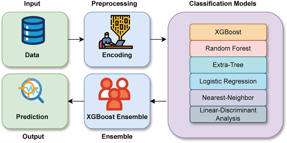
Figure 4. Flowchart of Ensemble-based Method used in the XGBoost algorithm Method WebHarvy (2022).

Here, $f(x)$ denotes the ensemble prediction, $M$ is the number of models, $w_i$ are the weights, and $f_i(x)$ are the individual model predictions. The given model adopts stacking, a popular ensemble technique that uses predictions from various models (first layer) which includes (Chen and Guestrin, 2016), random forest (Breiman, 2001), extremely randomized trees(Geurts et al., 2006), logistic regression (Fisher, 1936), nearest neighbor (Cover and Hart, 1967), and linear discriminant analysis (LDA) (Guisan et al., 2002) as input and a second layer of a single XGBoost classifier for ensembling.

The first layer trains multiple classifiers on the dataset. Each model, $f_i(x)$, produces a prediction, and these predictions are then stacked together as shown in Equations 12–13:

$P=\left[p_1,p_2,\dots ,p_M\right](12)$

here $p_i$ is the prediction of the $i$-th model.

The second layer is responsible for training the final model (e.g., XGBoost) on the stacked predictions $P$ to form the final prediction:

$f\left(x\right)=g\left(P\right)(13)$

here $g$ is the second-layer model.

The ensemble’s performance is assessed using the ROC-AUC and a confusion matrix. It measures the area under the Receiver Operating Characteristic curve, representing the model’s ability to discriminate between positive and negative classes.

3 Results and discussion

3.1 Overview of results

This study used a Graph Attention Network (GAT) to predict lead contamination levels in Flint, Michigan, focusing on contamination thresholds between 5 and 15 ppb. Our model performed well, with an Area Under the Curve (AUC) of 0.93, precision of 71.55%, and recall of 93.77%. In contrast, the XGBoost implementation had an AUC of 0.66, indicating its limitations in capturing complex spatial and relational data patterns.

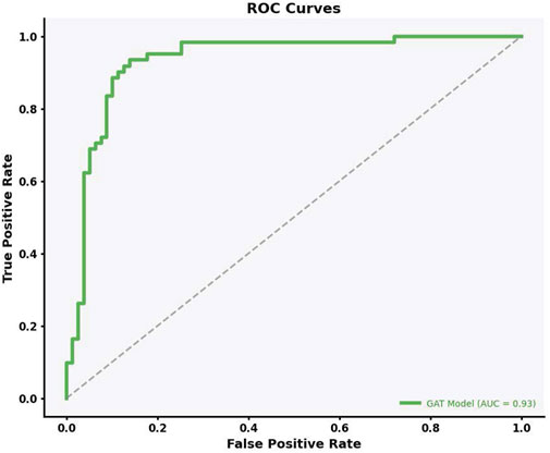
These results highlight the effectiveness of GAT in modeling lead contamination, especially in incorporating spatial features like parcel adjacency and housing proximity. Figure 5 illustrates the ROC curve for our model tested on the test dataset. The model, incorporates data from both the parcel layer and the Zillow data, achieving an impressive Area Under the Curve (AUC) of 0.93. This AUC value, combined with its proximity to the top-left corner of the graph, demonstrates the model’s efficiency in classification, indicated by a high TPR and a low FPR.

Figure 5

Figure 5. True positive vs. False positive rates ROC curve for GAT Model.

3.2 Comparative analysis with existing literature

We conducted a comparative analysis with key studies in the field to contextualize our findings within broader lead contamination research. This comparison underscores the progress achieved by our GAT model and its strengths in using spatial and relational data for better predictive performance. Abernethy et al. (2016) used an ensemble method to identify lead service lines in Flint, achieving an accuracy of 0.677. Although their approach demonstrated the potential of ensemble methods helping to identify lead, our GAT model’s AUC of 0.93 indicates a significant improvement. This suggests the importance of incorporating spatial and relational features, which are key strengths of GAT. Similarly, Goovaerts (2019) used a multivariate geostatistical approach (cokriging) to predict water lead levels, achieving an AUC of 0.76. Cokriging effectively captures spatial variability by integrating multiple data sources. Despite this, our GAT model achieved a higher AUC. While Goovaerts’ work offers very valuable insights into data integration, our results show that graph based modeling might provide a robust framework for predicting lead contamination. Mulhern et al. (2023) applied Bayesian Networks (BN) to predict lead risk, achieving an AUC of 0.74. Their method was particularly good at identifying high-risk facilities with clustered contamination. However, our GAT model showed higher AUC and recall, reflecting its ability to identify contaminated parcels more effectively. GAT’s capacity to model complex spatial relationships gives it broader applicability, particularly in urban areas where contamination is influenced by neighboring properties. In the study by Early Warning Systems (Khaksar Fasaee et al., 2022), Bayesian classifiers and Ensemble Decision Trees (EDT) were used to predict lead contamination in private water systems, achieving an AUC of 0.77 and recall of 75%. Although these models were effective, especially when incorporating household-level features, our GAT model achieved a higher AUC and recall. Overall, these comparisons show that our GAT model not only achieves high performance but also addresses some of the limitations in previous methods. By effectively integrating spatial and relational data, our approach improves predictive accuracy of the previous studies. This methodology offers a tool for lead contamination mitigation, ensuring resources are efficiently allocated to at risk households. The information presented in this study contribute to the ongoing research on lead contamination prediction and highlight the potential of using graph based methods in environmental health.

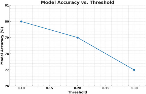
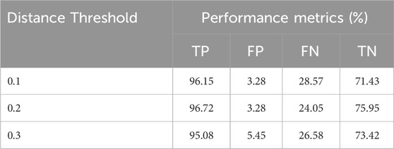
In Figure 6, the graph shows how the accuracy of the model changes as the distance threshold for connecting houses in the graph increases. Here, the threshold is the maximum distance between houses, in miles, that defines whether they are considered connected in the Graph Attention Network (GAT). At a 0.1-mile threshold, houses are connected only to their closest neighbors, and this setting yields the highest model accuracy (ACC), slightly above 80%. As the distance threshold increases to 0.3 miles, the model accuracy gradually decreases to just above 77%. This indicates that the model benefits from focusing on more local relationships. The trade off seen in the graph highlights the importance of selecting an appropriate threshold to find the right balance between connectivity and prediction quality. The confusion matrix results for the different thresholds are summarized in Table 3.

Figure 6

Figure 6. GAT model accuracy across different threshold.

Table 3

Table 3. Performance metrics based on distance threshold GAT model.

3.3 Ensemble learning with XGBoost

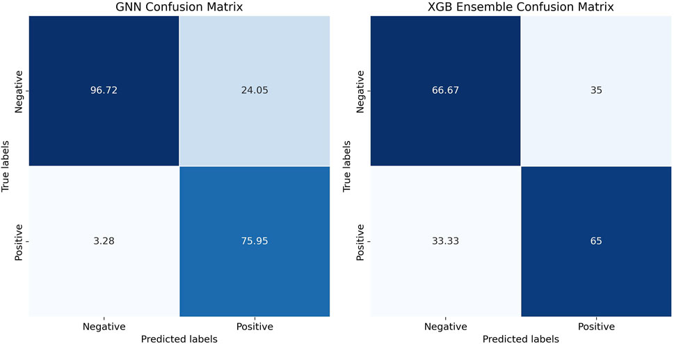
In addition to our evaluation of the GAT model, we compared the performance with an ensemble learning approach using the XGBoost method, a gradient-boosted decision tree algorithm, which was previously used by Abernethy et al. (2016). Ensemble models like XGBoost combine multiple individual models to achieve better predictive performance compared to individual models. XGBoost, in particular, has gained recognition for its ability to handle large and unbalanced datasets effectively. Abernethy et al. (2016) employed a model to identify lead service lines in Flint, reporting an accuracy of 67.7% and a log loss of 0.054. In our study, the XGBoost model achieved an accuracy of 70.0%, a precision of 65.57%, and a recall of 66.67%. While these results were comparable to those reported by Abernethy and Yang, the GAT model performed better across all key metrics. Specifically, the GAT model achieved an AUC of 0.93, a precision of 71.55%, and a recall of 93.77% Table 4. This demonstrates that the GAT model was better in identifying and correctly labeling homes that might have lead contamination. The confusion matrix in Figure 7 further illustrates the classification performance of the GAT model, showing the distribution of correct and misclassified predictions for both models. The main reason for this difference is that GAT can better leverage relationships between neighboring houses, which appears to be crucial for predicting lead contamination accurately. XGBoost, in contrast, focuses more on the volume and diversity of data without directly incorporating spatial relationships, which could explain why the GAT model proved to be effective.

Table 4

Table 4. Performance Metrics for Lead Contamination Prediction Models.

Figure 7

Figure 7. Confusion matrix comparison for model performance.

Although the GAT model had higher accuracies than XGBoost, XGBoost model still has strengths, such as its resistance to overfitting and scalability, which is a common advantage of gradient-boosted models. This was particularly useful in our case, where the dataset contained a lot of features. Moreover, the XGBoost model offered insights into which features were important, such as Housing Age and Property Address Street, which were also identified as significant by the GAT model. While GAT uses the spatial relationships between houses, XGBoost did well with the volume and variety of data. This difference explains their varying performance. In situations where spatial relationships are not the most critical aspect, XGBoost might still be a good alternative or complement to GAT. Future research could also explore combining both models to see if that improves its accuracy.

3.4 Performance comparison of GAT and XGBoost across different contamination thresholds

To show the performance difference between GAT and XGBoost, we turned the classification into a binary problem, using different lead contamination thresholds (5 ppb, 10 ppb, and 15 ppb). The GAT model consistently had higher accuracies compared to the XGBoost across all thresholds.

3.5 Sensitivity analysis

To further evaluate (GAT) model, we conducted sensitivity analyses, including an assessment of the ROC curve across contamination thresholds and an examination of different spatial distance thresholds.

3.6 ROC curve analysis

The ROC curve was used to assess how well the GAT model balances sensitivity and specificity across different thresholds. The model achieved an AUC of 0.93, showing its ability to distinguish between contaminated and non-contaminated parcels. This performance was better than that of XGBoost (AUC: 0.66) and Bayesian Networks (AUC: 0.74), highlighting GAT’s effectiveness in handling imbalanced datasets and capturing spatial relationships. Figure 5 shows the ROC curve for the GAT model across multiple thresholds, while Figure 8 focuses specifically on classifier performance at the EPA action level of 15 ppb. The model’s proximity to the left-top corner in these curves indicates strong predictive accuracy. In practical terms, this means that the GAT model can identify contaminated households effectively while reducing misclassification, which is important for managing limited resources in lead mitigation efforts.

Figure 8

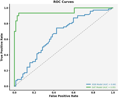
Figure 8. ROC Curve for Classifier 3 (15 ppb): Evaluating Model Performance at the EPA Action Level. This curve demonstrates the model’s ability to distinguish between houses with lead contamination levels above and below the EPA action threshold of 15 ppb.

3.7 Spatial distance threshold analysis

To complement the ROC curve analysis, we also evaluated how different spatial distance thresholds affected recall and precision. The GAT model was tested with thresholds ranging from 0.1 to 0.3 miles, which represented different levels of connectivity within the graph. At a 0.1-mile threshold, the model achieved the highest recall (93.77%), ensuring that most contaminated parcels were identified. Increasing the threshold to 0.3 miles slightly reduced recall but improved precision. This trade off highlights the spatial sensitivity of the model and the importance of selecting appropriate thresholds for specific public health goals. While spatial threshold analysis offers useful insights for optimizing the graph structure, the ROC curve analysis remains the primary metric for evaluating overall model performance. The ROC curve effectively summarizes the trade off between sensitivity and specificity across different decision thresholds.

3.8 Practical applications and implications

In public health contexts, such as the Flint water crisis, accurate predictive models are crucial for safety. A model that can predict lead levels in residential water helps guide interventions, ensuring that resources are directed to the areas that need them most. The aim is not just to achieve good accuracy but to reduce health risks for residents. Traditional methods often struggle to capture the spatial dependencies in lead contamination data. The GAT model effectively uses these spatial relationships, which allows for a better understanding of how contamination spreads. Future work could explore hybrid models that combine GAT with statistical approaches, like cokriging, for more predictive accuracy. Additionally, the model’s predictions can be used to help strategize local interventions, ensuring efficient use of resources.

3.9 Relative variable influence

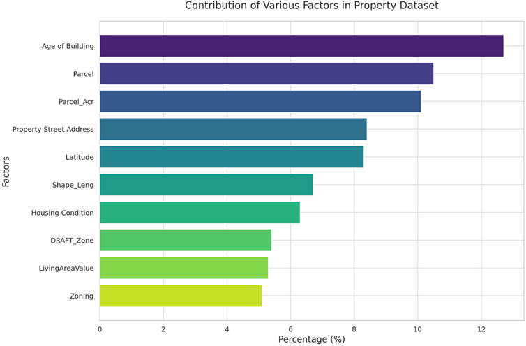
In our research utilizing the GAT framework, we aimed to pinpoint key node features crucial for predicting homes at risk for lead contamination in water. It is important to note that the identified risk factors do not directly imply causation of lead contamination but are useful in differentiating parcels with a higher likelihood of unsafe lead levels. By applying the GAT framework, which is effective in handling relational data, we identified features such as the Age of Building, Property Address, Zoning, and Parcel as significant predictors. For instance, older buildings may have outdated plumbing that increases lead risk. These findings could lead to more targeted inspections and informed policy-making aimed at reducing lead contamination.

To explain the importance of each feature, we used GraphLIME, a local interpretable model-agnostic explanation method tailored to Graph Neural Networks. This method approximates the complex GNN model with a simpler, interpretable model for a specific node’s neighborhood. By perturbing the node features and observing the changes in the model’s output, we determined the importance score of each feature:

$I\left(f_i\right)=P\left(F\right)-P\left(F\backslash f_i\right)$

Where.

• $I(f_i)$ represents the importance score of feature $f_i$.

• $F$ is the complete set of features.

• $F\backslash f_i$ denotes the feature set excluding feature $f_i$.

Figure 9 shows the top important features as determined by our model’s output.

Figure 9

Figure 9. Top-predicting features.

Interestingly, our model revealed that some features traditionally considered important in lead contamination studies, such as Longitude Elevation, were less influential. This suggests a more complex role for geographic factors in lead contamination risk. Features like DraftZone and Housing Condition (HCond 2012) were more influential, emphasizing the importance of housing-related factors in lead risk. Even features that might seem less critical, such as Living Area Value and Parcel Acres, provide valuable context for understanding potential lead contamination sources. These insights can help guide targeted and effective interventions, shaping policies to prioritize resources for mitigating lead contamination.

3.10 Practical applications and broader context

The accuracy of predictive models in public health, particularly in scenarios like Flint’s lead crisis, has real implications for community safety. Correctly predicting lead levels in residential water allows authorities to plan interventions and allocate resources efficiently, focusing on the most vulnerable areas first.

The ROC curves in Figure 10 provide additional insight into the model’s classification performance at these thresholds. Our model consistently performed better than traditional methods in identifying contaminated homes, particularly across different lead thresholds ($>5$, $>10$, $>15$ ppb), as shown in Figure 11. The use of GAT captures spatial dependencies and relationships effectively, something that traditional methods, including Flint’s ensemble models, struggled to do. The attention mechanism of GAT allows it to weigh neighboring nodes differently, which leads to a better understanding of how lead contamination spreads or clusters.

Figure 10

Figure 10. ROC curves of true positive rates vs. false positive rates for the models with different thresholds. The first figure represents a threshold of >5 ppb, the second figure represents a threshold of >10 ppb, and the third figure represents a threshold of >15 ppb. These figures illustrate the model's ability to distinguish between contaminated and non-contaminated houses at different levels of lead concentration.

Figure 11

Figure 11. Our algorithm’s binary classification performance comparisons for different thresholds with different baseline algorithms. The left figure shows overall performance, while the middle and right figures show performance for each class (contaminated vs. non-contaminated) for thresholds ($>5,>10,>15$ ppb).

The success of integrating alternative data sources, such as Zillow information, highlights the potential for unconventional but relevant data to provide additional context in a crisis. It also shows the importance of collaboration between public entities and private data holders to enrich available data and improve model accuracy. Future research could explore how other data sources might be leveraged in similar contexts, whether for pollution monitoring, understanding disease spread, or urban planning.

3.11 Applicability beyond the USA

Although this model was developed using U.S. data, applying it elsewhere requires adjusting for local regulations, infrastructure, and data availability. Different regions may have stricter or more lenient lead thresholds, unique sources of contamination (e.g., industrial pollution or agricultural runoff), and varying monitoring practices. Retraining or recalibrating the model with local data is often necessary to capture these differences accurately. In areas lacking centralized water quality records, community-driven sampling or municipal reports might be required. The lessons from Flint demonstrate how data-driven approaches can support public health interventions, reinforcing the importance of predictive models that integrate machine learning with real-world applications.

4 Conclusion

The Flint water crisis is a clear reminder of the serious consequences that happen when environmental and public health problems collide. This study shows that Graph Attention Networks (GAT) can be a valuable tool to help predict lead contamination more accurately, thanks to its ability to capture complex spatial relationships. However, it’s important to note that the GAT model is just one part of the solution it complements other efforts and supports better decision making.

One of the key findings of this study is the identification of features that are strong predictors of high lead levels in homes, even without knowing the exact composition of Lead Service Lines (LSLs). This is crucial information that can help policymakers and community members target high-risk areas, allocate resources more efficiently, and take action to protect public health.

Technical Implications: The GAT model has shown strong potential in improving how we assess water quality risks, helping us identify high-risk areas more effectively. Municipalities could use similar models to focus their efforts on the neighborhoods most vulnerable to lead contamination. Future monitoring systems should look to integrate such graph-based tools to get ahead of issues before they escalate.

Policy Implications: The findings suggest that incorporating predictive models like GAT can help public health authorities make better use of limited resources. By pinpointing areas most likely to face lead contamination, actions can be prioritized to prevent health risks before they become widespread. Additionally, this research highlights the value of using diverse data sources—like real estate information—to enrich monitoring efforts. Collaborations between public and private entities can make datasets more robust and improve the ability to address contamination proactively.

Limitations: While the GAT model offers many benefits, it’s not without its limitations. The model relies heavily on the quality and availability of data as well as scalability. Users of this model should be mindful of these constraints and recognize that the model should be seen as a guiding tool rather than a definitive solution. Continuous data collection, validation, and refinement of the model are needed to improve accuracy and reduce uncertainties.

The findings from this research are not just relevant to Flint. The approach used in this study can be applied in other areas, like urban planning, pollution monitoring, and public health research. By bringing together public health agencies, local governments, and private data providers, we can create more effective datasets that ultimately lead to safer communities.

In conclusion, addressing public health issues like lead contamination requires a combination of advanced technology and practical policy changes. By using tools like GAT alongside careful policymaking and resource allocation, we can tackle challenges like the Flint water crisis more effectively. The future focus should be on refining these models, improving data quality, and extending these approaches to other communities to better manage lead contamination risks on a broader scale.

Data availability statement

Publicly available datasets were analyzed in this study. This data can be found here: https://www.michigan.gov/flintwater/water-infrastructure-projects/monitoring/wqa-flint-dist/city-of-flint-distribution-system-monitoring-data-expanded-data-set.

Author contributions

RA: Conceptualization, Data curation, Formal Analysis, Funding acquisition, Investigation, Methodology, Project administration, Resources, Software, Supervision, Validation, Visualization, Writing–original draft, Writing–review and editing. YB: Conceptualization, Data curation, Investigation, Visualization, Writing–review and editing. CS: Visualization, Writing–review and editing. MP: Data curation, Writing–review and editing. PK: Formal Analysis, Funding acquisition, Project administration, Resources, Writing–review and editing. BL: Funding acquisition, Writing–review and editing, Project administration. MA: Conceptualization, Data curation, Formal Analysis, Funding acquisition, Investigation, Methodology, Project administration, Resources, Software, Supervision, Validation, Visualization, Writing–original draft, Writing–review and editing.

Funding

The author(s) declare that financial support was received for the research and/or publication of this article. This research was supported by a grant from the National Science Foundation (NSF) under the Smart and Connected Community (SCC) program. The grant, approximately valued at $2.5 million USD, is titled “SCC-IRG Track 1: Community Based Approach to Address Contaminants in Drinking Water using Smart Cloud-Connected Electrochemical Sensors,” with the award number 2230180.

Conflict of interest

The authors declare that the research was conducted in the absence of any commercial or financial relationships that could be construed as a potential conflict of interest.

Publisher’s note

All claims expressed in this article are solely those of the authors and do not necessarily represent those of their affiliated organizations, or those of the publisher, the editors and the reviewers. Any product that may be evaluated in this article, or claim that may be made by its manufacturer, is not guaranteed or endorsed by the publisher.

Supplementary material

The Supplementary Material for this article can be found online at: https://www.frontiersin.org/articles/10.3389/fenve.2025.1488965/full#supplementary-material

References

Abernethy, J., Anderson, C., Dai, C., Farahi, A., Nguyen, L., Rauh, A., et al. (2016). Flint water crisis: data-driven risk assessment via residential water testing. doi:10.48550/arXiv.1610.00580

CrossRef Full Text | Google Scholar

Agency, U. E. P. (2023). Lead regulations.

Google Scholar

Aldhyani, T. H. H., Al-Yaari, M., Alkahtani, H., and Maashi, M. (2020). Water quality prediction using artificial intelligence algorithms. Appl. Bionics Biomechanics 2020, 1–12. doi:10.1155/2020/6659314

PubMed Abstract | CrossRef Full Text | Google Scholar

Bae, Y., Pasteris, J. D., and Giammar, D. E. (2020a). The ability of phosphate to prevent lead release from pipe scale when switching from free chlorine to monochloramine. Environ. Sci. and Technol. 54, 879–888. doi:10.1021/acs.est.9b06019

PubMed Abstract | CrossRef Full Text | Google Scholar

Bae, Y., Pasteris, J. D., and Giammar, D. E. (2020b). Impact of iron-rich scale in service lines on lead release to water. AWWA Water Sci. 2, e1188. doi:10.1002/aws2.1188

CrossRef Full Text | Google Scholar

Bae, Y., Pasteris, J. D., and Giammar, D. E. (2020c). Impact of orthophosphate on lead release from pipe scale in high ph, low alkalinity water. Water Res. 177, 115764. doi:10.1016/j.watres.2020.115764

PubMed Abstract | CrossRef Full Text | Google Scholar

Bahdanau, C. K. D., and Bengio, Y. (2015). Neural machine translation by jointly learning to align and translate. doi:10.48550/arXiv.1409.0473

CrossRef Full Text | Google Scholar

Bai, T., and Tahmasebi, P. (2023). Graph neural network for groundwater level forecasting. J. Hydrology 616, 128792. doi:10.1016/j.jhydrol.2022.128792

CrossRef Full Text | Google Scholar

Blackhurst, M. (2021). Identifying lead service lines with field tap water sampling. ACS ES&T Water 1, 1983–1991. doi:10.1021/acsestwater.1c00227

CrossRef Full Text | Google Scholar

Breiman, L. (2001). Random forests. Mach. Learn. 45, 5–32. doi:10.1023/A:1010933404324

CrossRef Full Text | Google Scholar

Chen, T., and Guestrin, C. (2016). Xgboost: a scalable tree boosting system. CoRR. doi:10.48550/arXiv.1603.02754

CrossRef Full Text | Google Scholar

Chojnacki, A., Dai, C., Farahi, A., Shi, G., Webb, J., Zhang, D. T., et al. (2017). “A data science approach to understanding residential water contamination in flint,” in Proceedings of the 23rd ACM SIGKDD international Conference on knowledge Discovery and data mining (ACM). doi:10.1145/3097983.3098078

CrossRef Full Text | Google Scholar

Cornwell, D. A., Brown, R. A., and Via, S. H. (2016). National survey of lead service line occurrence. J. AWWA 108, E182–E191. doi:10.5942/jawwa.2016.108.0086

CrossRef Full Text | Google Scholar

Cover, T., and Hart, P. (1967). Nearest neighbor pattern classification. IEEE Trans. Inf. Theory 13, 21–27. doi:10.1109/tit.1967.1053964

CrossRef Full Text | Google Scholar

Devine, C., Mello, K., DeSantis, M., Schock, M., Tully, J., and Edwards, M. (2024). Calcium phosphate precipitation as an unintended consequence of phosphate dosing to high-ph water. Environ. Eng. Sci. 41, 171–179. doi:10.1089/ees.2023.0190

CrossRef Full Text | Google Scholar

Doré, E., Lytle, D. A., Wasserstrom, L., Swertfeger, J., and Triantafyllidou, S. (2020). Field analyzers for lead quantification in drinking water samples. Crit. Rev. Environ. Sci. Technol. 51, 2357–2388. doi:10.1080/10643389.2020.1782654

PubMed Abstract | CrossRef Full Text | Google Scholar

Fawcett, T. (2006). An introduction to roc analysis. Pattern Recognit. Lett. 27, 861–874. doi:10.1016/j.patrec.2005.10.010

CrossRef Full Text | Google Scholar

Fisher, R. A. (1936). The use of multiple measurements in taxonomic problems. Ann. Eugen. 7, 179–188. doi:10.1111/j.1469-1809.1936.tb02137.x

CrossRef Full Text | Google Scholar

Floridi, L., and Taddeo, M. (2016). What is data ethics? Philosophical Trans. R. Soc. A Math. Phys. Eng. Sci. 374, 20160360. doi:10.1098/rsta.2016.0360

PubMed Abstract | CrossRef Full Text | Google Scholar

García-Timermans, C., Malfroot, B., Dierendonck, C., Mol, Z., Pluym, T., Waegenaar, F., et al. (2023). Pilot-scale drinking water distribution system to study water quality changes during transport. npj Clean. Water 6, 52. doi:10.1038/s41545-023-00264-8

CrossRef Full Text | Google Scholar

Geurts, P., Ernst, D., and Wehenkel, L. (2006). Extremely randomized trees. Mach. Learn. 63, 3–42. doi:10.1007/s10994-006-6226-1

CrossRef Full Text | Google Scholar

Goovaerts, P. (2019). Geostatistical prediction of water lead levels in flint, Michigan: a multivariate approach. Sci. Total Environ. 647, 1294–1304. doi:10.1016/j.scitotenv.2018.07.459

PubMed Abstract | CrossRef Full Text | Google Scholar

Guisan, A., Edwards, T. C., and Hastie, T. (2002). Generalized linear and generalized additive models in studies of species distributions: setting the scene. Ecol. Model. 157, 89–100. doi:10.1016/s0304-3800(02)00204-1

CrossRef Full Text | Google Scholar

Gurewitsch, R. (2019). Pb-predict: using machine learning to locate lead plumbing in a large public water system

Google Scholar

Hajiseyedjavadi, S., Blackhurst, M., and Karimi, H. A. (2020). A machine learning approach to identify houses with high lead tap water concentrations. Proc. AAAI Conf. Artif. Intell. 34, 13300–13305. doi:10.1609/aaai.v34i08.7040

CrossRef Full Text | Google Scholar

Hajiseyedjavadi, S., Karimi, H. A., and Blackhurst, M. (2022). Predicting lead water service lateral locations: geospatial data science in support of municipal programming. Socio-Economic Plan. Sci. 82, 101277. doi:10.1016/j.seps.2022.101277

CrossRef Full Text | Google Scholar

Han, H., Pan, D., Li, Y., Wang, J., and Wang, C. (2020). Stripping voltammetric determination of lead in coastal waters with a functional micro-needle electrode. Front. Mar. Sci. 7. doi:10.3389/fmars.2020.00196

CrossRef Full Text | Google Scholar

Hensley, K., Bosscher, V., Triantafyllidou, S., and Lytle, D. A. (2021). Lead service line identification: a review of strategies and approaches. AWWA Water Sci. 3, 1–19. doi:10.1002/aws2.1226

PubMed Abstract | CrossRef Full Text | Google Scholar

Khaksar Fasaee, M. A., Pesantez, J., Pieper, K. J., Ling, E., Benham, B., Edwards, M., et al. (2022). Developing early warning systems to predict water lead levels in tap water for private systems. Water Res. 221, 118787. doi:10.1016/j.watres.2022.118787

PubMed Abstract | CrossRef Full Text | Google Scholar

Kuhn, M., and Johnson, K. (2013). Applied predictive modeling. Springer. doi:10.1007/978-1-4614-6849-3

CrossRef Full Text | Google Scholar

Li, G., Bae, Y., Mishrra, A., Shi, B., and Giammar, D. E. (2020). Effect of aluminum on lead release to drinking water from scales of corrosion products. Environ. Sci. and Technol. 54, 6142–6151. doi:10.1021/acs.est.0c00738

PubMed Abstract | CrossRef Full Text | Google Scholar

Lin, Y., Qiao, J., Bi, J., Yuan, H., Gao, H., and Zhou, M. (2022). “Hybrid water quality prediction with graph attention and spatio-temporal fusion,” in 2022 IEEE international conference on systems, man, and cybernetics (SMC), 1419–1424. doi:10.1109/SMC53654.2022.9945293

CrossRef Full Text | Google Scholar

Lobo, G., Laraway, J., and Gadgil, A. (2022). Identifying schools at high-risk for elevated lead in drinking water using only publicly available data. Sci. Total Environ. 803, 150046. doi:10.1016/j.scitotenv.2021.150046

PubMed Abstract | CrossRef Full Text | Google Scholar

Lopez, K. G., Xiao, J., Crockett, C., Lytle, C., Grubbs, H., and Edwards, M. (2024). Zinc orthophosphate can reduce nitrate-induced corrosion of lead solder. ACS ES&T Water 4, 3153–3162. doi:10.1021/acsestwater.3c00786

PubMed Abstract | CrossRef Full Text | Google Scholar

Martin, S., and Griswold, W. (2009). Human health effects of heavy metals. Environ. Sci. Technol. Briefs Citizens, 1–6. doi:10.4236/jep.2017.811077

CrossRef Full Text | Google Scholar

Michigan.gov (2023). Michigan lead safe home program.

Google Scholar

Mulhern, R. E., Kondash, A., Norman, E., Johnson, J., Levine, K., McWilliams, A., et al. (2023). Improved decision making for water lead testing in u.s. child care facilities using machine-learned bayesian networks. Environ. Sci. and Technol. 57, 17959–17970. doi:10.1021/acs.est.2c07477

PubMed Abstract | CrossRef Full Text | Google Scholar

News21 (2023). Millions consumed potentially unsafe water in the last 10 years.

Google Scholar

Ni, R., Chu, X., Liu, R., Shan, J., Tian, Y., and Zhao, W. (2024). Chromium immobilization and release by pipe scales in drinking water distribution systems: the impact of anions. Sci. Total Environ. 906, 167600. doi:10.1016/j.scitotenv.2023.167600

PubMed Abstract | CrossRef Full Text | Google Scholar

Pan, W., Pan, C., Bae, Y., and Giammar, D. (2019). Role of manganese in accelerating the oxidation of pb(ii) carbonate solids to pb(iv) oxide at drinking water conditions. Environ. Sci. and Technol. 53, 6699–6707. doi:10.1021/acs.est.8b07356

PubMed Abstract | CrossRef Full Text | Google Scholar

Pasteris, J., Bae, Y., Giammar, D., Dybing, S., Yoder, C., Zhao, J., et al. (2021). Worth a closer look: Raman spectra of lead-pipe scale. Minerals 11, 1047. doi:10.3390/min11101047

CrossRef Full Text | Google Scholar

Potash, B., Brew, J., Loewi, A., Majumdar, S., Reece, A., Walsh, J., et al. (2015). “Predictive modeling for public health,” in Proceedings of the 21th ACM SIGKDD international conference on knowledge discovery and data mining. doi:10.1145/2783258.2788629

CrossRef Full Text | Google Scholar

Sandvig, A., Kwan, P., Kirrmeyer, G., Maynard, B., Mast, D., Trussell, R., et al. (2008). Contribution of service line and plumbing fixtures to lead and copper rule compliance issues. Denver, CO: Water Research Foundation.

Google Scholar

Sarr, S. O. E. N., and Diallo, A. (2018). “Factextract: automatic collection and aggregation of articles and journalistic factual claims from online newspaper,” in 2018 fifth international conference on social networks analysis, management and security (SNAMS) IEEE, 336–341.

Google Scholar

Sawan, S., Maalouf, R., Errachid, A., and Jaffrezic-Renault, N. (2020). Metal and metal oxide nanoparticles in the voltammetric detection of heavy metals: a review. TrAC Trends Anal. Chem. 131, 116014. doi:10.1016/j.trac.2020.116014

CrossRef Full Text | Google Scholar

Trueman, B. F., Camara, E., and Gagnon, G. A. (2016). Evaluating the effects of full and partial lead service line replacement on lead levels in drinking water. Environ. Sci. and Technol. 50, 7389–7396. doi:10.1021/acs.est.6b01912

PubMed Abstract | CrossRef Full Text | Google Scholar

Vaswani, A., Shazeer, N., Parmar, N., Uszkoreit, J., Jones, L., Gomez, A. N., et al. (2017). Attention is all you need. Adv. Neural Inf. Process. Syst. doi:10.48550/arXiv.1706.03762

CrossRef Full Text | Google Scholar

Veličković, P., Cucurull, G., Casanova, A., Romero, A., Liò, P., and Bengio, Y. (2018). “Graph attention networks,” in International conference on learning representations (ICLR).

Google Scholar

Vlachou, E., Margariti, A., Papaefstathiou, G. S., and Kokkinos, C. (2020). Voltammetric determination of pb(ii) by a ca-mof-modified carbon paste electrode integrated in a 3d-printed device. Sensors 20, 4442. doi:10.3390/s20164442

PubMed Abstract | CrossRef Full Text | Google Scholar

Vrahatis, A. G., Lazaros, K., and Kotsiantis, S. (2024). Graph attention networks: a comprehensive review of methods and applications. Future Internet 16, 318. doi:10.3390/fi16090318

CrossRef Full Text | Google Scholar

WebHarvy (2022). What is web scraping.

Google Scholar

Zanfei, A., Brentan, B. M., Menapace, A., Righetti, M., and Herrera, M. (2022). Graph convolutional recurrent neural networks for water demand forecasting. Water Resour. Res. 58, e2022WR032299. doi:10.1029/2022WR032299

CrossRef Full Text | Google Scholar

Zhou, J., Cui, G., Hu, S., Zhang, Z., Yang, C., Liu, Z., et al. (2020). Graph neural networks: a review of methods and applications. AI Open 1, 57–81. doi:10.1016/j.aiopen.2021.01.001

CrossRef Full Text | Google Scholar

Zillow (2023). Zillow: real estate, apartments, mortgages and home values.

Google Scholar