Electricity markets price projection: an innovative approach for risk assessment based on a convolution algorithm. ERCOT case study

In electricity markets, the determination of future energy prices is relevant for risk assessment associated with investment projects in new generation capacity and in the evaluation of risks associated with the operation of the market whose mitigation requires increasing the operating reserves in the electrical system. Traditional methods for estimating energy prices in electricity markets are based on using simulation models that represent the expected future operation of the electricity market. These models fail to estimate market prices when the greatest uncertainty that affects the system reserve is due to the unavailability of the generation fleet and the volatility of the production of renewable wind and solar generation. This document presents a new methodology that allows determining energy prices in electricity markets that is considered superior to traditional methods. It is an innovative approach for risk assessment in power markets with high participation of renewable generation (wind, solar) and thermal generation. The model determines market prices considering the randomness in the typical production of renewable generation and the randomness in the availability of thermal power plants due to forced failures. Market prices are determined through a convolution algorithm applied to the probability functions that characterize energy demand, the randomness in the production of renewable generation, and the availability of thermal generation units. The calculation methodology is considered superior to Monte Carlo-type methodologies used by other simulation programs. A case study is included where the electricity market of Texas USA (ERCOT) is simulated and comparing the market prices resulting from the new simulation model with the real market prices recorded in the year 2022. The market prices determined by the proposed new methodology provide relevant information for consumers to evaluate energy purchase alternatives correctly and for investors in new generation capacity to determine the profitability of their projects. In particular, it allows the correct determination of energy prices in periods of scarcity allowing storage media (BESS) to be correctly sized so that they can provide a quickly managed reserve and thus improve the reliability of the electrical system.

1 Introduction

In many countries around the world, the production and consumption of electrical energy are organized through Wholesale Electricity Markets (WEM). Market rules establish the mechanisms based on which generation dispatch is determined each hour. The hourly generation dispatch seeks to supply the demand of each hour with an adequate quality of service at the lowest possible cost.

To meet the aforementioned objectives, the operation of the market is carried out by Independent System Operators (ISO).

One of the most relevant activities of the ISO is to schedule the production of all generators in advance so that they know (for the next hours) the expected operation of their units. This will allow them to carry out the required actions so that the generation units are available to produce energy according to the operation programming carried out by the ISO.

The programming of the operation carried out by the ISO typically covers one week (168 h), and is also carried out one day before (Day Ahead) and during the actual operation (real-time). In systems with a high hydraulic generation component, long-term operation programming is also carried out (typically for the next 2 years), which aims to program the operation of hydro plants and the use of their reservoirs with high regulation capacity. that exist in the electrical system.

To carry out the programming of the operation, the ISOs use computer programs as tools that solve the optimization problem (minimum cost) with the technical restrictions that exist in the electrical system (transmission limits, start and stop times of generators, the safety conditions of the system, etc.) (Roald et al., 2023; Allan et al., 1981; Pereira and Pinto, 1985).

To determine the operation schedule, the simulation models use information from the electrical system: forecast hourly demand, available power from the generators, intermittent renewable generation (ERV-Wind/Solar), transmission system configuration, and the transmission capacity limits of each circuit. It is also necessary to know the production costs of the generators (fuel and O&M costs). In some markets, generators offer a price at which they are willing to produce electrical energy. It is also required to know the shortage price that is activated when the existing reserve in the system is reduced below the minimum required to guarantee the normal supply of demand. It is highlighted that the scarcity price is usually much higher than the variable production cost of thermal generators.

The programming of the operation is carried out under conditions of uncertainty. The main variables that affect the operation programming are (i) evolution of hourly demand, (ii) availability of the generation units, (iii) hourly production of the ERV generators, and in systems with high participation of hydro generation, the inflows to hydro plants reservoirs, activation of restrictions imposed by the transmission system.

As a result, Day-Ahead dispatch scheduling generally differs from Real-Time operation.

1.1 Market prices

At the end of each day, the ISO determines the energy prices in the market for each hour of the day. The price of energy (Market Price) is equal to the price offered by the generator that was dispatched at the time and whose price offered is the maximum. When the hourly generation reserve is lower than the minimum required, the energy price reflects the scarcity price.

The ISO does not have, as part of its obligations, to make projections of future market prices. This implies that market agents (generators, consumers) do not have information about expected future market prices that allow them to make decisions about investments, energy purchases/sales, risk assessments, etc.

To solve this problem, market agents usually use the same computer programs (simulation model) that the ISO uses to program the market operation or other software with similar characteristics (Jedrzejewski et al., 2022).

These programs determine the expected operation of the generation fleet in the future (within a defined time horizon) and the expected marginal cost of generation in each hour [Lagrange multiplier for the (Generation = Demand) constraint]. To take into account the existing uncertainty regarding the variables that affect economic dispatch and energy prices, random draws (Monte Carlo algorithm) are usually used to determine the availability of generating units. In the case of electrical systems with high participation of hydraulic generation, the simulation programs consider different hydraulic contributions to the hydro plants, and calculation algorithms are used that allow optimizing the use of water within the calculation horizon.

In electricity markets with reduced participation of hydro generation (such as the ERCOT of Texas-USA) (Hegar, n.d.), the greatest source of uncertainty that affects the projection of market prices are (i) the availability of thermal generation units, (ii) the production of the generators ERV, and (iii) the occurrence of operating conditions with low generation reserves that activate scarcity prices. It is noted that since the scarcity price is much higher than the production cost of the generators, the activation of low reserve conditions has the effect of significant increases in market prices.

Figure 1 presents the hourly variations [Demand (h) – Demand (h-1)] of the demand in the ERCOT (red curve), for the year 2023. It is observed demand variations are limited to ±5,000 MW.

Figure 1

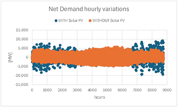
Figure 1. Hourly variations of Net Demand, with and without Solar PV generation. Source: data from ERCOT.

The hourly variations in demand that are supplied by thermal generation (net demand) show a greater variation (greater volatility) with maximums of ±10,000 MW, which is directly associated with the volatility in solar production.

The energy transition expected in the future will increase the share of renewable generation in the electricity markets. As an example, at the ERCOT it is projected to increase the installed solar PV capacity by 200% (+30 GW; source: Potomac Economics) in the next 5 years. This will increase the volatility in demand that is supplied by thermal generation (Net Demand), resulting in significant variations in market prices, putting the normal supply of demand at risk, and increasing the need for adequate forecasts of the expected future evolution of market prices (Llarens et al., 2022).

This document proposes a new methodology to determine market prices under the aforementioned conditions which is considered superior to Monte Carlo-type methods. The proposed methodology is based on using a convolution algorithm of independent statistical functions to determine the expected production of the generating units and the energy market prices. The convolution algorithm allows consideration in the calculation of all possible operating states resulting from contingencies in the generation fleet, resulting in a better quantification of the effect of scarcity prices on market prices.

A case study is included where the proposed new methodology is applied to determine market prices in ERCOT of TX, and results are compared with the real prices of the year 2022.

2 Market prices considering uncertainty in generators' availability

In a thermal generation fleet, the availability of the generation units determines the power available in the market to supply the demand. A conventional generator has two possible operation states (Available and unavailable). A Combined Cycle type generator composed of three generation units (2xTG+ST) has three operating states. A thermal generation fleet composed of N conventional generators has 2^N possible operating states.

As an example, Figure 2 show the possible operating states corresponding to a generation fleet composed of three conventional generation units. The operating states are 2³ = 8. A “0” is indicated when the operating unit is unavailable and a (1) when the generating unit is available. For each state, the total power results from the sum of the power of the available units. Each state has a probability of occurrence (pT) determined by the Failure Rate (q) of each generating unit.

$\begin{array}{r}ifg(i)=0,p(i)=q(i),p(i)=(1-q(i))\\ pT=p(1)\times p(2)\times p(3)\end{array}$

Figure 2

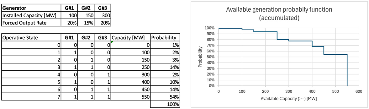
Figure 2. Available generation probability function.

i: each generator

g(i) = (0, 1): operative state of the generator (i)

q(i): generator failure rate (i)

Figure 2 shows the resulting probability function. The example considers three conventional generators (G#1, G#2, G#3). There are therefore 8 (=23) possible operating states for the three generators. In the table, the operating state of each generator is indicated by 0 or 1 (0; unavailable; 1: available). The total available capacity is the sum of the available capacities of each generator in each state. The probability of each state results from the product of the probability that each generator is available or unavailable. The cumulative probability function (Figure 2 right) shows the probability of having a total power greater than the value of the abscissa.

It is observed that the probability of having the total power of the generation fleet available is 54% and that there is a probability (>0) that the generation fleet has an available power equal to zero.

The production of each generator that supplies a certain demand at minimum cost results from the economic dispatch of generation. For this purpose, the price at which the generators produce energy (VPC), the demand to be supplied and the cost of insufficient reserve (NSEC) must be defined.

Figure 3 shows an example of calculation considering all the operating states of the three generators.

Figure 3

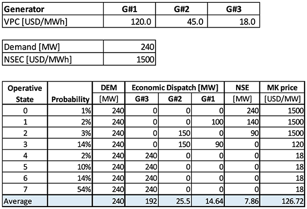
Figure 3. Operative states probability function. In this example, the market price of each state corresponds to the marginal cost of generation, including the cost of not having enough reserve to supply all demand.

To carry out the economic dispatch of generation, the demand to be supplied (240 MW) and the generation available in each operating state is considered. The available generation is ordered by their increasing variable production costs (VPC; fuel cost+O&M). The cheapest generators are dispatched first until the demand is met. When the available generation capacity is insufficient to supply the demand, the residual demand determines the unsupplied demand (NSE). The market price for each operating state is equal to the VPC of the unit with the highest VPC dispatched; when there is NSE, the market price is equal to the NSEC.

It is observed:

• For the same demand (240 MW), there are different dispatches of the generating units and correspondingly different values of the Market Price.

• Even though the total installed power of the generation fleet (550 MW) is much higher than the demand to be supplied there is a probability (>0) of not being able to supply all of the demand.

• Events with a very low probability of occurrence (low reserve) determine high market prices.

• The market price probability function has very different P50 (18 USD/MWh) and Paverage (126.72 USD/MWh) values.

2.1 Conclusion

For a conventional generation fleet (with G generators) in which the availability of the generators is dependent on fortuitous events (failures), there are N = 2^G possible operating states. Therefore, the market prices will have associated an probability function (p(i)) that depends on the failure rate of the generating units. In the example before the Market Prices probability function is shown in the Figure 4. The average market price is 126.72 [USD/MW].

Figure 4

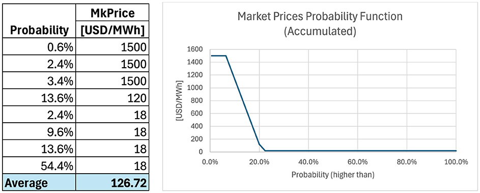
Figure 4. Market prices probability function.

In Electricity Markets, with high participation of thermal generators, typically the average market price resulting from all possible operative states is considered to be representative of the most probable projected value of market prices. In the following, the projected average market price will be referred to as the “expected market price – MkPe.”

Therefore, for a given demand to be supplied (240 MW in the example before) the expected market price (MkPe) resulting from the probability function (p(i)) is equal to 126.72 USD/MWh.

$\begin{array}{l}MkPe={\displaystyle \sum _{i=1}^N}p(i)\times MkPrice(i)\end{array}$

where,

i: each possible operating state

N: total number of possible operating states

p(i): Probability of state (i)

MkPrice (i): Market Price determined for the state (i)

MkPe: Expected Market Price.

The total operating cost ($TC) is also a probability function since it depends on the production (EG) and operative costs (VPC = fuel cost + O&M costs) of each generator and the cost of insufficient operating reserve (NSEC).

The NSEC represents the cost incurred by consumers when their demand cannot be met due to insufficient generation capacity. In electricity markets, the NSEC is established as part of the grid code nd is a key value for generation fleet expansion studies and reliability studies.

The expected total supply cost ($TCe) for consumers results from the product of the average production of the generators valued at their respective production cost (VPC) plus the cost of insufficient reserve.

$\begin{array}{l}\$TCe={\displaystyle \sum _{j=1}^G}EG{e}_j\times VP{C}_j+NSEe\times NSEC\\ EG{e}_j={\displaystyle \sum _{i=1}^N}p(i)\times E{G}_j(i)\\ NSEe={\displaystyle \sum _{i=1}^N}p(i)\times NSE(i)\end{array}$

Where

$TCe [USD]: total expected supply cost

j: each generator

i: each operating state

G: number of generators

N: number of operating states

p(i): Probability of state (i)

EGj(i) [MWh]: energy generated by the generator (j), in the operating state (i)

NSE (i) [MWh]: energy not supplied in the operational state (i)

VPCj [USD/MWh]: variable production cost of the generator (j)

NSEC [USD/MWh]: cost of energy not served due to insufficient reserve

The expected total supply cost ($TCe) is an increasing function with the demand to be supplied, as seen in the Figure 5 for the example previously analyzed. The function is increasing because the greater the demand to be supplied, the more expensive generation units will be required to be dispatched, which increases the total supply cost.

Figure 5

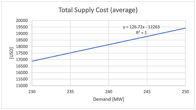
Figure 5. Total supply cost (average) function.

The expected Market Price (MkPe; 126.72), for a given demand (D0), is equal to the derivative of the expected total supply cost function (slope of the regression line) for D = D0. We can therefore determine market prices with the following expression:

$\begin{array}{l}MkPe\left(D0\right)=\frac{d}{dD}\$TCe\left(D\right)]forD=D0\end{array}$

This property allows us to determine market prices by evaluating total expected supply costs.

In the next point, a methodology is developed to determine the total expected supply cost using a convolution algorithm from which market prices will be determined.

3 Market's prices—convolution algorithm

In the electricity market, the demand and the available capacity of each generator at each moment can be considered as independent probability functions (f1, f2).

The demand for each hour (h) of the period (T) can be represented as a probability density function f1, where the probability of each demand value is equal to (1/T).

Figure 6 show an example of the calculation procedure for the f1 function considering T = 168 h (1 week). The hourly demand (Figure 6 left) is ordered from highest to lowest values, resulting in what is called a monotonic demand curve (Figure 6 right). Each demand value on the monotonic demand curve is assigned a probability (1/T = 1/168), resulting in the curve in the Figure 6 represents the cumulative probability function (F1) of the demand. The sum of all demand values times (1/T) equals the average demand for period T.

$\begin{array}{l}Dem(ave)={\displaystyle \sum _{i=1}^{i=T}}Dem(i)\times f1(i)=\frac{1}{T}\times {\displaystyle \sum _{h=1}^T}Dem(h)\end{array}$

Figure 6

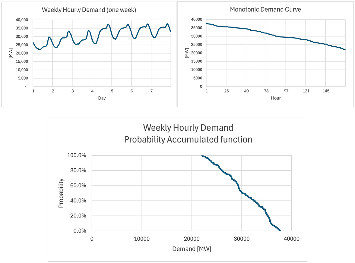
Figure 6. Hourly demand accumulated probability function.

The accumulated probability function F1 shows that the demand has a 0% probability of being greater than the maximum value (37,750 MW), it has a 100% probability (the 168 h of the week) of being greater than the minimum value (22,091 MW) and during the 50% of the time (84 h) the demand is <30,101 MW.

The probability function corresponding to a generator (f2) takes into account the possible operating states of the generator with their corresponding probabilities of occurrence. A conventional thermal generator has two possible operating states: (1) Available to produce energy with a power equal to its installed power, and (2) Unavailable. If the generator has a failure rate (q) the probability of being unavailable will be (q) and the probability of being available will be (1 – q). A Combined Cycle (CC) type thermal generator composed of three generating units (2xTG+1xST) will have 8 possible operating states (2^G where G = number of generating units).

Figure 7 show typical accumulated probability functions (F2) for a conventional thermal power plant and a Combined Cycle (CC) type thermal power plant. Figure 7 (left) corresponds to a conventional generator with an installed capacity of 200 MW and an Availability Rate of 85%. Figure 7 (right) corresponds to a CC generator composed of three units (2xTG+1xTV) where each unit has a capacity of 200 MW, a total capacity equal to 600 MW, and an availability rate of 85%.

Figure 7

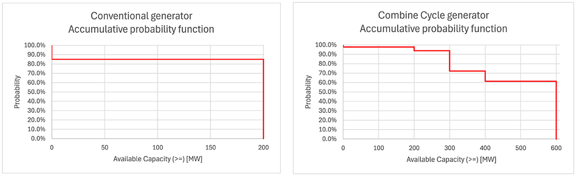
Figure 7. Thermal generators accumulated probability function (Conventional, Combine Cycle).

In both cases, an available power greater than the total installed capacity (200 MW, 600 MW) has a probability equal to zero, and there is a 100% probability that the available capacity is (≥0). A conventional generator has two operating states (available, and unavailable), correspondingly, The probability of having an available power (>0) is equal to the generator availability rate (85%). A CC-type generator has 8 (=23) possible operating states, the curve shows the probability considering all operating states.

3.1 Convolution algorithm

The convolution of discrete probabilistic functions is a mathematical operation used to find the probability distribution of the sum of two independent random variables (f1, f2). Convolution of discrete statistical functions is a fundamental operation in the analysis of discrete signals and systems. It is used to combine two discrete probability sequences to produce a third sequence that represents how one of the sequences superimposes on the other. It is widely used in various areas such as signal processing, statistics, optics, acoustics, engineering, and physics (Xu et al., 2023; Tsun, 2020).

The convolution procedure used to determine the production of each generator is shown in Figure 8. The demand to be supplied (monotonic curve) is shown in ❶. The evaluation period (T) is normalized to 1.0. To supply this demand, a conventional generator G1 is available, which has an unavailability rate (q1). The generator has two possible operating states: 1: Available, with probability (1 – q1), and 2: Unavailable, with probability q1.

Figure 8

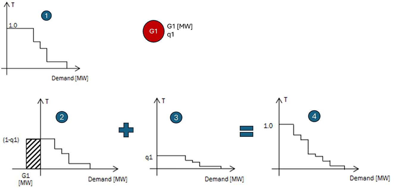
Figure 8. Procedure for determining the generation dispatch by convolution.

When G1 is available, part of the demand will be supplied by the generator. In ❷ the residual demand is indicated. The curve is equal to ❶ multiplied by (1 – q1) and shifted to the left G1[MW].

When G1 is unavailable the residual demand is ❸. The curve is equal to ❶ multiplied by (1 – q1).

The residual demand considering the two possible operating states of the generator is indicated in ❹. It is obtained by adding both curves ❷ and ❸.

The energy generated by G1 is the shaded portion of ❷ multiplied by T.

If other generators are available to supply the demand (G2, G3, GN), the procedure indicated above is repeated until all the generators have been considered. In each recursion, the initial demand ❶ is equal to the residual demand of the previous recursion ❹. In each recursion, the energy production of each of the generators is obtained as a result.

In the electrical systems, in each hour (h), the “net demand (ND)” is equal to the difference between the demand and the production of the generators.

$\begin{array}{l}\text{Net Demand }(\text{h})=\text{ Demand }(\text{h})+(-\text{ generation }(\text{h}))\end{array}$

The probability functions of demand (f1) and generator (f2) determine the Net Demand (ND), therefore ND is also a probability function (f3). Since f1 and f2 are independent probabilistic functions, the probability function f3 can be obtained by convolution of the functions f1 and f2.

$\begin{array}{r}{f}_3=f_1*f_2\\ f_3(z)={\displaystyle \sum _x}{f}_1(x)·f_2(z-x)\end{array}$

Where:

f1: probability density function of hourly demand, F1; accumulated distribution function

f2: probability density function of (− generation (h)), F2; accumulated distribution function

f3: probability density function of net demand, F1; accumulated distribution function

* is the convolution operator:

The concepts indicated above can be used to determine the production of the generators under conditions of uncertainty in the availability of the generating units and the average market prices of a period of interest (1 h, 1 day, a week, etc.).

The convolution algorithm allows determining the production of each generator (i). The resulting production will be the average power for the evaluated period. The calculation procedure is recursive as shown in Figure 9 considering that the system has “i” generators. In each recursion, the net demand probability function (f3) resulting from the convolution of the functions f1 and f2 is determined. Net Demand (ND(i)) is the residual demand after the generator (i) is dispatched. The net demand is determined for each recursion, which allows the production of each generator to be determined (by difference), and the energy that could not be supplied by the generators (NSE).

$\begin{array}{l}ND(0)={\displaystyle \sum _{j=1}^{DMax}}j\times f_{10}(j)\\ ND(i)={\displaystyle \sum _{j=1}^{DMax}}j\times f_{1i}(j)\\ G(i)=ND(i-1)-ND(i)\\ NSE={\displaystyle \sum _{j=1}^{DMax}}j\times f_{1NG}(j)\end{array}$

Figure 9

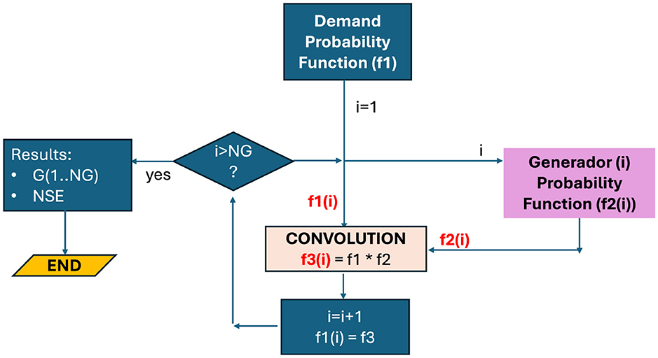
Figure 9. Block diagram of generation dispatch based on convolution algorithm applied to the demand and generation probability functions.

Below is the source code of a FORTRAN 77 program that allows carrying out the calculation indicated above for the following example where the production of three generators and the NSE are determined by convolution. The demand to be supplied has a maximum power of 15 MW (Figure 10).

Figure 10

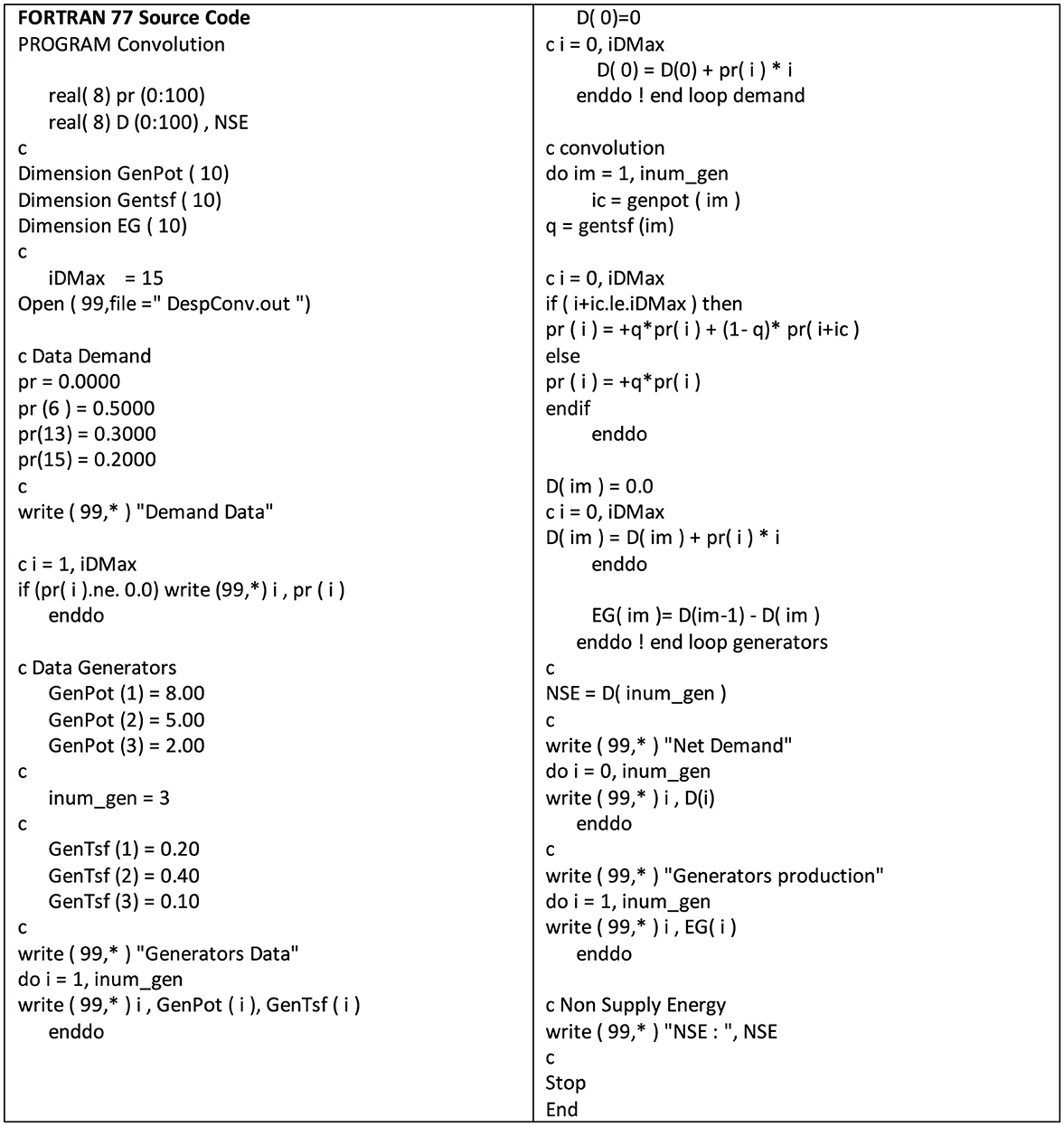
Figure 10. Fortran code for generation dispatch based on the convolution algorithm applied to the demand and generation probability functions.

Figure 11 show the results of the generation dispatch obtained by applying the convolution algorithm above described and the probability density functions corresponding to the demand [f1(0)] and the net demand probability functions after the dispatch of each generator [f1(1), f1(2), f1(3) respectively].

Figure 11

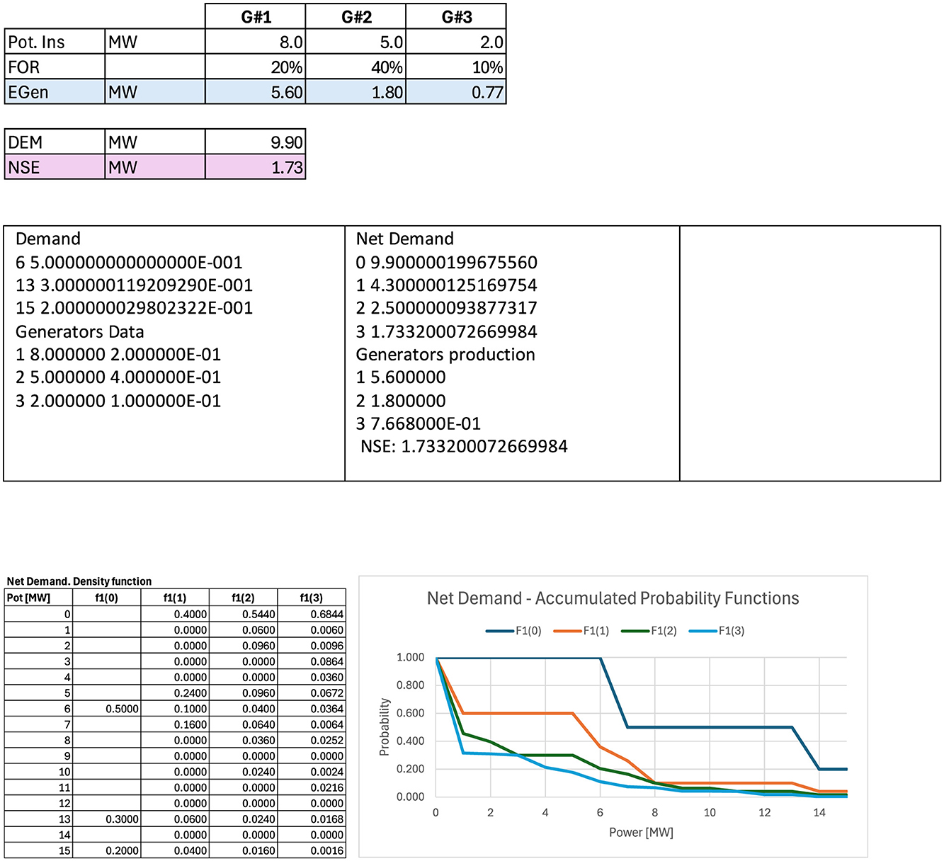
Figure 11. Example of generation dispatch based on convolution algorithm.

3.2 Determination of market prices

Once the average production of each generator and the average NSE are calculated, using the convolution algorithm described in the previous point, it is possible to determine the production cost of each generator ($G(i)), the cost of the NSE ($NSE) and the total cost ($TC) resulting from the sum of the costs indicated above considering all generators (NG).

$\begin{array}{l}\$G(i)=VPC(i)\times EG(i)\\ \$NSE=NSEC\times NSE\\ \$TC={\displaystyle \sum _{i=1}^{NG}}\$G(i)+\$NSE\end{array}$

If the order in which the convolution is performed considers the generators ordered according to their variable production costs (VPC; first the cheapest generator, followed by the highest cost generators – MERIT LIST), the total cost determined will be the MINIMUM average operating cost for the evaluated period.

By repeating the procedure indicated above, increasing the demand (ΔD = 1MW), a new total cost corresponding to the increased demand ($TCI) will be obtained.

The expected market price (MkPe) of the evaluated period results from the difference of both total costs indicated above.

$\begin{array}{l}MkPe=\$TCI-\$TC\end{array}$

4 EMPP simulation model

Based on the theoretical concepts described in the previous points, the Electricity Markets Price Projection Software (EMPP) simulation model was developed, whose functional diagram is shown in Figure 12. The model allows determining market prices in electricity markets with a high participation of thermal and renewable wind/solar generation such as ERCOT in Texas—USA. Prices are determined by the periods required by the user.

Figure 12

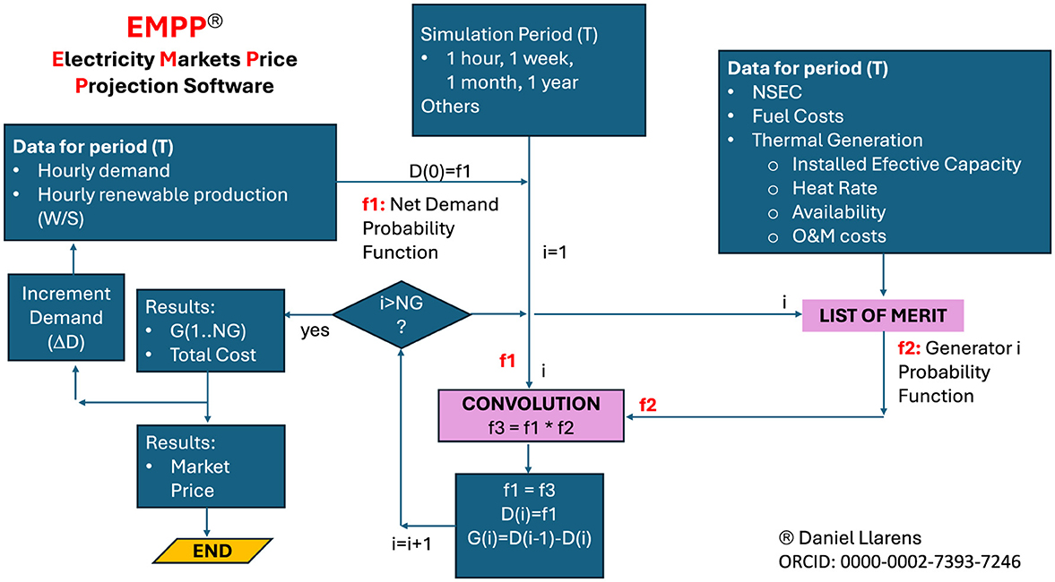
Figure 12. EMPP Software block functional diagram.

The model considers as data the total hourly demand of the market, the hourly production of the wind and solar renewable generators, the characteristics of the thermal generation fleet (installed capacity, availability of the generating units, production costs), and the NSEC of the market. An example of using the software is presented in this document.

The model determines the following results for the evaluated period:

• Production of each generating unit (renewable, thermal)

• NSE

• Total supply cost

• Average market prices.

The data required by the EMPP model are the following:

1. Simulation period (T): corresponds to the period for which the expected market price is required to be determined. It can be 1 h, 168 h of a week, all hours of the month, a particular hour of each month, or any other period.

2. Hourly demand [MW]: demand of the electricity market for each hour of the period T

3. Renewable generation [MW]: total renewable generation (wind, solar, others) of the electricity market for each hour of the period T

4. Thermal generators data: Type (TG, CC), Effective Installed Power at the plant location site, Availability, Thermal Efficiency, Fuel Cost, O&M Costs

The calculation process is recursive.

Step 1: The net hourly demand is determined [Net Demand (h) = Demand (h) – Renewable Generation (h)]. The probability function corresponding to Net Demand is f1(0).

Step 2: The (N) existing thermal generators are ordered in ascending order of their VPC, the cheapest first (MERIT LIST)

Step 3: The counter (i) that identifies each generator in the MERIT LIST is initialized. (I = 1) corresponds to the cheapest generator.

Step 4: The probability function f2 corresponding to the generator (i) is determined.

Step 5: The convolution between the probability functions (f1, f2) is performed. As a result, the probability function f3 corresponding to the residual demand resulting from the dispatch of generator i is obtained, f1(i) = f3

Step 6: Generator recursion: Steps 4 and 5 are repeated until I = N, in each recursion the function f1(i) will be obtained as a result

Step 7: With the functions f1(0), f1(1), f1(2), …, f1(N) the residual demand as a result of the dispatch of each generator is determined

$\begin{array}{l}D(0)={\displaystyle \sum _{j=1}^{DMax}}j\times f_1(0)(j)\end{array}$

$\begin{array}{l}D(1)={\displaystyle \sum _{j=1}^{DMax}}j\times f_1(1)(j)\end{array}$

$\begin{array}{l}D(N)={\displaystyle \sum _{j=1}^{DMax}}j\times f_1(N)(j)\end{array}$

Step 8: The expected production of each generator (i) and the NSE are determined by difference

$\begin{array}{r}G1=D(0)-D(1)\\ G2=D(1)-D(2)\\ Gi=D(i-1)-D(i)\\ NSE=D(N)\end{array}$

Step 9: With the production of each generator, its corresponding VPC, and the NSEC, the Reference total cost of supply ($TCR) is determined.

$\begin{array}{l}\$TCR={\displaystyle \sum _{i=1}^{NG}}G(i)\times VPC(i)+NSE\times NSEC\end{array}$

Step 10: Demand Recursion. System Demand is increased by ΔD = 1 MW and steps 1 to 8 are repeated. The result is the total supply cost corresponding to the increased demand ($TCI)

Step 11: The expected market price in period T (MkPe) is:

$\begin{array}{l}\text{MkPe}=(\$TCI)-(\$TCR)\end{array}$

4.1 Limitations of the EMPP model

1. The EMPP model does not allow for optimizing the generation of hydro-power plants. This is the reason why it cannot be used directly to determine market prices in hydrothermal systems where the hydro generation component is important (e.g. Colombia, Brazil). In electrical systems, such as PJM-USA, Mexico, where the hydro generation component is <20%, it is possible to use EMPP in combination with traditional simulation models to determine market prices. The calculation is done in two steps: Step 1: using traditional models the hydro generation is determined. Step 2: with EMPP, market prices are determined considering, as data, the hydro production pattern (hourly production) determined in Step 1.

2. The EMPP model considers generation and demand located in the same node of the transmission system. Therefore, the EMPP model does not include the restrictions imposed by the transmission network on the economic dispatch of generation. As a result, market prices must be considered as representative of the market without considering possible effects (losses, congestion) on the prices of each node.

4.2 Comparison with Monte Carlo methodology

Next, the market prices determined using EMPP are compared with prices determined using the Monte Carlo methodology (random draws).¹

Figure 13 present the data considered for the simulation. In this example, the demand to be supplied is 7,000 MW, the same throughout the simulation period. The generation fleet includes 100 generating units with a total installed capacity of 12,560 MW. The NSEC is equal to 4,000 USD/MWh.

Figure 13

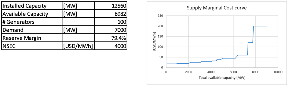
Figure 13. Demand and generation data used for the comparison.

Using EMPP the result average market price is

$\begin{array}{l}\text{MkPe}=93.28USD/\text{M}\text{W}\text{h}\end{array}$

Using the Monte Carlo methodology, the average market price is very dependent on the number of draws and the seed used to initialize the random draw. Figure 14 presents the average price determined for 10 different seeds considering 1,000 draws. Significant differences are observed between the results (up to 15.9 USD/MW) even for a significant number of draws.

Figure 14

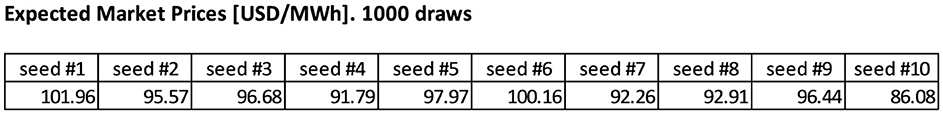
Figure 14. Monte Carlo methodology. Expected market prices [USD/MWh]. 1,000 draws.

Figure 15 presents the average market price determined for 3 different seeds as a function of the number of random draws. For a reasonable number of draws (200), a high dispersion in average prices is observed. For a large number of draws (1,000), the average prices determined by Monte Carlo methods converge to the value determined by convolution using EMPP model.

Figure 15

Figure 15. Monte Carlo methodology. Average market prices function of # of draws.

The aforementioned results show that it is not convenient to use a methodology based on Monte Carlo to estimate market prices in systems with a high participation of thermal generation considering a reasonable number of draws to limit the simulation times.

It is highlighted that the simulation carried out using EMPP produces exact results since it considers all possible operating states (associated with the availability of the generation units) and that the computing time required to perform the simulation is not significant.

5 ERCOT case study

The Electric Reliability Council of Texas (ERCOT) provides electricity service in Texas (USA) to more than 90% of the state's consumers. The demand in 2022 was 525.6 TWh with a maximum demand of 78,325 MW.

To supply the demand, ERCOT has an installed generation capacity (Dec-2022) made up of 120,570 MW of independent power producers (IPP) plus 28,329 MW owned by distribution companies (Utilities). The generation capacity is mainly thermal plus renewable generation. The main fuel used for thermal generation is Natural Gas, abundant in the state of TX. Figure 16 show the generation capacity by type.

Figure 16

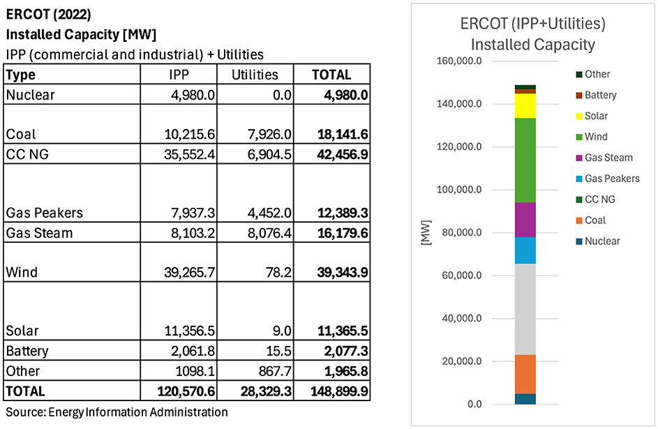
Figure 16. ERCOT. Generation installed capacity by type.

ERCOT determines generation dispatch using offers of available capacity and prices done by generators. Every hour, the generators that offer the lowest prices are dispatched until the hourly demand is met, complying with operational safety criteria and systems constraints.

As a result of the operation, ERCOT determines the market prices for the Day Ahead Market (DAM) and the Real Time Market (RTM). The prices in each hour are equal to the price offered by the generator with the highest price offered that was dispatched in the hour (marginal offer). Typically, Market Prices show seasonal variations associated with variations in demand; they are maximum in the summer months when system demand is maximum. Also, variations are observed between MDA and MTR prices mainly due to random effects of variations in demand and availability of generation units.

When the electrical system operates in conditions of low generation reserve, market prices are determined by the curve in Figure 17, reaching 5,000 USD/MWh when the reserve is <3,000 MW (scarcity prices).

Figure 17

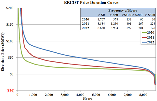
Figure 17. ERCOT. Energy prices duration curves. Source: Potomac Economics.

The Figure 17 shows the duration curves of market prices for the years 2020–2022. Very high prices are observed in at least 1,000 h/year, which are associated with low generation reserves that force the dispatch of high-cost generation units and eventually the activation of scarcity prices. This demonstrates that the effects of generation availability are relevant in ERCOT in recent years, affecting the risks faced by investments in new generation capacity and the operational security of the electric system.

In 2023, the problems of low reserve reserves continued

ERCOT said in May it has enough power to meet peak demand through the summer, unless an unlikely confluence of events happens. If a big coal or natural gas power plant goes offline, there's less wind and solar energy available than forecast and there's intense heat, ERCOT may have to implement rolling blackouts for a couple hours to stabilize the grid.

Source: Houston Chronicle, June 22, 2023.

Unlike many other electricity markets, in ERCOT there is no Capacity Balancing Market. Therefore, the generators that operate in the market do not have a remuneration associated with their Installed/Firm Capacity. This makes the market energy price the only economic signal to promote efficient investments in new generation capacity, making the correct estimation of market prices very important.

In the future, it is expected that the operational problems of low reserves will increase due to the combined effect of the unavailability of generation units and the expected increase in wind/solar generation which are characterized by a high volatility of its production.

Under the operating conditions mentioned above, the risk assessment analysis associated with market prices will be a relevant aspect in the economic evaluation of new generation projects and for the purchase of energy through long-term contracts.

5.1 ERCOT's market prices: case study

The future operating conditions at ERCOT are expected to result in very high volatility of Market Prices due to the activation of scarcity prices in low reserve hours.

As mentioned in the previous points, traditional simulation models fail in determining market prices when scarcity prices are frequently activated since they cannot correctly simulate all the expected operating states of the generation fleet. To obtain approximate results, thousands of draws are required, which makes the simulation unfeasible due to the times required to do the simulations and subsequent processing of the information that arises from the model.

Using traditional simulation models, the only viable alternative is to project market prices, in markets such as ERCOT, using the available capacity of the generation units and their respective variable production costs (not a Monte Carlo methodology). This methodology produces good results when the generation reserve is adequate.

The simulation model described in this document based on the use of a convolution algorithm (EMPP model) takes into account all operating states which allows us to determine market prices considering the generation reserve that exists at each moment due to the random effects associated with demand variations, availability of generation units, intermittency of wind/solar generation.

As an example, Figures 18, 19 compares, for year 2022, the ERCOT prices, year 2022 (source: Potomac Economics; black dash line) with the prices resulting from:

• A traditional simulation model based on the available capacity of the generation units (red line).

• EMPP model based on a convolution algorithm (blue line).

Figure 18

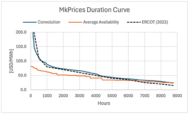
Figure 18. Energy prices duration curves comparison.

Figure 19

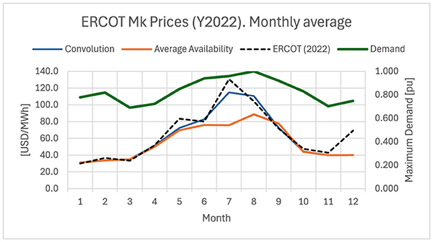
Figure 19. Energy prices monthly average comparison.

It is highlighted

• EMPP model produces market prices similar to the real ones, resulting in a price duration curve and monthly average prices similar to the real one.

• The price duration curve based on the traditional model has significant differences with the real curve for prices with a duration of <3,000 h (prices during scarcity hours).

• In the summer months (Jun–Aug), when demand is maximum and generation reserves are minimum, the average prices projected by EMPP are similar to the real ones, while those projected with traditional models are less showing significant differences.

It is noted that due to the structural characteristics of ERCOT, energy prices in the summer months are always high as a way of producing economic signals for the expansion of the generation fleet. Since traditional models cannot adequately represent the economic signals associated with scarcity, they will always produce results that do not allow the identification of the need for expansion of the generation fleet. On the other hand, EMPP evaluates all the operating conditions resulting from the unavailability of the generation units, resulting in the correct projection of energy prices mainly under conditions of scarcity.

6 Conclusions

The determination of future market prices is relevant to the functioning of electricity markets since it allows generators and consumers to define their strategies regarding energy purchases and investments in new generation capacity. It is also relevant to guarantee the operational security of the electrical system through investments in storage media (BESS) that allow for mitigating the adverse effects of intermittency in the production of wind/solar generators. The energy transition planned in the future, which will lead to an increase in renewable generation, will increase the need for adequate forecasts of the expected future evolution of market prices.

The operation simulation models that are used by system operators (ISO) and market agents allow for estimating the expected future production of each generator. They are also suitable for estimating market prices in electrical systems with high participation of hydraulic generation (e.g. Brazil, Colombia), where the main uncertainty is the water inflows to the system reservoirs.

These models generally fail to determine market prices in electricity markets where the main uncertainty is the availability of the generation units. This is the case of electrical systems with a high participation of renewable wind, solar, and thermal generation. An example of this type of system is ERCOT market (Texas, USA).

Traditional models use Monte Carlo-type techniques to perform a statistical analysis of market prices by making random draws to determine the availability of generation units. The results obtained with this methodology demonstrate that the determined prices are highly variable depending on (i) the seed used by the random number generator, and (ii) the number of draws carried out. Thousands of draws are typically required for the prices to tend to the expected average value, which increases the computing time without guaranteeing that the result obtained is correct.

A new simulation model called EMPP is presented in this document, which allows for determining the minimum cost generation dispatch and the average market prices expected in a time interval. To this end, the model uses a convolution algorithm to evaluate all possible operating states in electrical systems with a high participation of renewable generation and thermal generation.

Test simulations carried out with the EMPP show that the prices determined are similar to those obtained with Monte Carlo techniques only when conventional models a large number of draws are carried out (>>10,000). Therefore, using the EMPP correct results can be obtained with minimal computer system requirements and at reasonable computer time.

Test simulations of the ERCOT (Texas-USA electricity market) show that the prices obtained with EMPP are close to the real ones, while the prices determined with traditional models show a significant difference during the hours in which the electrical system has low generation reserves, where Market prices are affected by scarcity prices.

Based on the aforementioned, EMPP model is considered superior to traditional simulation models for risk assessment analysis in electricity markets where the main source of uncertainty is the availability of the generator units due to combined effects of contingencies in the generation fleet and variations in the primary resource of wind/solar generation.

The use of EMPP provides significant information for the development of renewable generation projects, mainly Solar-PV generation. EMPP allows determining the expansion of thermal generation and storage media (BESS) required to ensure safe and low-cost operation of the electrical system. So, the possibility of developing Solar-PV generation is conditioned by thermal expansion since the total cost must be minimized. Therefore, EMPP also allows sizing the existing market space for the development of Solar-PV generation.

6.1 Potential improvements for the EMPP model

The provision of ancillary services (operating reserves) is required in electricity markets as a way of ensuring the safe operation of the electrical system. The determination of operating reserves is the result of an optimization process where the cost of the reserve is compared with the cost of supplying the demand plus the NSE avoided by having the operating reserve.

The EMPP model can be improved to determine optimum operative reserves using the results of NSE and the market prices for different values of the operating reserve, which allows the supply of the demand safely and at minimum total cost (co-optimization).

Data availability statement

The datasets presented in this article are not readily available because confidentiality. Requests to access the datasets should be directed to ZGFuaWVsLmxsYXJlbnNAZ3J1cG9tZS5jb20=.

Author contributions

DL: Conceptualization, Data curation, Formal analysis, Investigation, Methodology, Project administration, Software, Validation, Writing – original draft, Writing – review & editing.

Funding

The author(s) declare that no financial support was received for the research, authorship, and/or publication of this article.

Acknowledgments

The author thanks Eng Jose Luis Cabello and Eng. Matias Fluxa for the support received in developing the calculation tool included in the EMPP model. The author also thanks the National University of La Plata, Argentina, a free public institution, for having trained them in the field of engineering and mathematics.

Conflict of interest

The author declares that the research was conducted in the absence of any commercial or financial relationships that could be construed as a potential conflict of interest.

Publisher's note

All claims expressed in this article are solely those of the authors and do not necessarily represent those of their affiliated organizations, or those of the publisher, the editors and the reviewers. Any product that may be evaluated in this article, or claim that may be made by its manufacturer, is not guaranteed or endorsed by the publisher.

Footnotes

1. ^Monte Carlo analysis is a method that uses random numbers to simulate a phenomenon or process that has uncertainty or variability. The seed is a number that determines the starting point of the random number generator, which produces the random numbers used in the simulation. The seed is important for the reproducibility and validity of the Monte Carlo analysis, as different seeds can produce different results.

References

Allan, R. N., Leite da Silva, A. M., Abu-Nasser, A. A., and Burchett, R. C. (1981). Discrete convolution in power system reliability. IEEE Trans. Reliab. R-30, 452–456. doi: 10.1109/TR.1981.5221166

Crossref Full Text | Google Scholar

Hegar, G. (n.d.). Texas Controller of Public Accounts. Available at: COMPTROLLER.TEXAS.GOV.

Google Scholar

Jedrzejewski, A., Lago, J., Marcjasz, G., and Weron, R. (2022). Electricity price forecasting: the dawn of machine learning. IEEE Power Energy Mag. 20, 24–31. doi: 10.1109/MPE.2022.3150809

Crossref Full Text | Google Scholar

Llarens, D., Souilla, L., Masiriz, S. A., and Lestard, G. R. (2022). Variable Renewable Energy. How the Energy Markets Rules Could Improve Electrical System Reliability. London: IntechOpen. doi: 10.5772/intechopen.107062

Crossref Full Text | Google Scholar

Pereira, M. V. F., and Pinto, L. M. V. G. (1985). Stochastic optimization of a multireservoir hydroelectric system: a decomposition approach. Water Resour. Res. 21, 779–792. doi: 10.1029/WR021i006p00779

Crossref Full Text | Google Scholar

Roald, A., Pozo, D., Papavasiliou, A., Molzahn, D. K., Kazempour, J., and Conejo, A. (2023). Power systems optimization under uncertainty: A review of methods and applications. Electr. Power Syst. Res. 214(Part A):108725. doi: 10.1016/j.epsr.2022.108725

Crossref Full Text | Google Scholar

Tsun, A. (2020). “Chapter 5. Multiple random variables,” in Probability & Statistics with Applications to Computing 5.5. (Paul G. Allen School of Computer Science & Engineering, University of Washington), 158–228. Available at: https://courses.cs.washington.edu/courses/cse312/20su/files/student_drive/5.5.pdf

Google Scholar

Xu, J., Hu, B., Zhang, P., Zhou, X., Xing, Z., and Hu, Z. (2023). Regional electricity market price forecasting based on an adaptive spatial–temporal convolutional network. Front. Energy Res. 11:1168944. doi: 10.3389/fenrg.2023.1168944

Crossref Full Text | Google Scholar