A configuration and scheduling optimization method for integrated energy systems considering massive flexible load resources

Introduction: With the increasing demand for energy utilization efficiency and minimization of environmental carbon emissions in industrial parks, optimizing the configuration and scheduling of integrated energy systems has become crucial. This study focuses on integrated energy systems with massive flexible load resources, aiming to maximize energy utilization efficiency while reducing environmental impact.

Methods: To model the uncertainties in wind and solar power outputs, we employed three-parameter Weibull distribution models and Beta distribution models. Flexible loads were categorized into three types to match different electricity consumption patterns. Additionally, an enhanced Kepler Optimization Algorithm (EKOA) was proposed, incorporating chaos mapping and adaptive learning rate strategies to improve search scope, convergence speed, and solution efficiency. The effectiveness of the proposed optimization scheduling and configuration methods was validated through a case study of an industrial park located in a coastal area of southeastern China.

Results: The results show that using three-parameter Weibull distribution models and Beta distribution models more accurately reflects the variations in actual wind speeds and solar irradiance levels, achieving peak shaving and valley filling effects and enhancing renewable energy utilization. The EKOA algorithm significantly reduced curtailment rates of wind and solar power generation while achieving substantial economic benefits. Compared with other operation modes of hydrogen, the daily average cost is reduced by 12.92%, and external electricity purchases are reduced by an average of 20.2 MW h/day.

Discussion: Although our approach shows potential in improving energy utilization efficiency and economic gains, this paper only considered hydrogen energy for single-use pathways and did not account for the economic benefits from selling hydrogen in the market. Future research will further incorporate hydrogen demand response mechanisms and optimize the output of integrated energy systems from the perspective of spot markets. These findings provide valuable references for relevant engineering applications.

1 Introduction

Globally, the escalating ecological environmental degradation and climate change issues have prompted countries to accelerate the transformation of their energy structures. Faced with the dual challenges of increasing energy demand and mounting pressure to reduce carbon emissions, traditional single-energy systems can no longer meet the modern society’s needs for low-carbon, environmentally friendly, and secure energy supply. As a result, the development of integrated energy systems with multi-energy coupling has become a key path for achieving energy transition (Peng et al., 2024). By integrating various forms of energy, such as electricity, heat, cooling, and gas, and optimizing resource allocation, integrated energy systems enhance energy utilization efficiency and offer significant economic and environmental benefits. These systems are gradually becoming a research focus in the energy field.

With the rise of integrated energy systems, the optimization of configuration and scheduling has become one of the key research areas in energy studies. This issue involves how to reasonably allocate various energy facilities within integrated energy systems and achieve efficient energy management through intelligent scheduling algorithms (Yang et al., 2023). Given the intermittency and uncertainty of renewable energy power generation, as well as multi-energy flow coupling issues, optimization of configuration and scheduling has become crucial for improving environmental friendliness and energy systems’ economic efficiency. Therefore, exploring optimization algorithms and scheduling strategies suitable for different scenarios to achieve optimal performance of integrated energy systems has become an urgent research need.

Several methods have been proposed in the literature for optimizing scheduling in multi-energy complementary systems. For instance, regarding wind-solar coupling systems, Xue et al. (2019) used the two-parameter Weibull distribution and Beta distribution for wind and solar uncertainty modeling. However, the simulation results were unsatisfactory, with a significant gap between actual and simulated wind power output. Akgül et al. (2016) proposed a system optimization model with the goal of minimizing investment and operational costs, and used Particle Swarm Optimization (PSO) to solve the model. However, the solution’s accuracy was insufficient, and the algorithm was prone to falling into local optima. Jiang et al. (2024) considered climate uncertainty factors and constructed a regional integrated energy system scheduling model with the goal of minimizing daily operational costs. Yang et al. (2022) proposed a dynamic economic scheduling model that took into account the depth of charge and discharge and battery life of energy storage systems. Using a genetic algorithm, they optimized the output of various power sources. Experimental results showed that the method could help integrated energy systems better adapt to complex real-world situations, improving energy utilization efficiency while extending the lifespan of energy storage systems. However, the algorithm had slow optimization speed and struggled to handle high-dimensional optimization problems. Therefore, to improve the solution efficiency of scheduling optimization problems of integrated energy systems, there is an urgent need to research more effective solution methods.

The Kepler Optimization Algorithm (KOA) (Von Loeper et al., 2020) is a novel and reliable metaheuristic algorithm (Yuan et al., 2024) based on Kepler’s laws of planetary motion, which treats the position, mass, gravity, and orbital velocity of the planets as four basic operators. In this algorithm, each planet and its position represent a candidate solution, which is randomly updated relative to the current best solution during the optimization process, thereby enabling a more effective exploration and utilization of the search space. Although KOA has demonstrated good performance in solving continuous optimization problems, it still faces challenges in handling high-dimensional optimization problems and achieving rapid convergence. To further improve the algorithm’s convergence speed and accuracy, it is crucial to make enhancements to the algorithm. Therefore, this paper focuses on how to strengthen the Kepler Optimization Algorithm to better adapt to more complex and large-scale optimization problems, thus better meeting the needs of practical applications.

This paper mainly studies the configuration and scheduling optimization problem of integrated energy systems. Firstly, a mathematical model of the integrated energy system is established, and a wind-solar uncertainty model is introduced to better represent the fluctuations in wind and solar output. Secondly, considering the volatility of renewable energy output, hydrogen storage is introduced to enhance the stability of the regional integrated energy system. Furthermore, a low-carbon flexible planning and scheduling model is established based on the multi-energy combined supply benefits and the costs of curtailed wind and solar energy to improve the absorption level of renewable energy and maximize the economic benefits of the integrated energy system. An enhanced Kepler Optimization Algorithm is introduced to improve the model’s solution efficiency. Finally, the effectiveness of the proposed planning and scheduling method is verified through an example of an industrial park in the southeastern coastal region of China.

Based on the above research the innovations of this paper are as follows:

(1) Firstly, in terms of flexible model modeling, the existing studies usually focus on a single type of flexible loads (transferrable loads or dispatchable loads), whereas in this paper, we have comprehensively included non-interruptible loads for the first time, transferrable loads and dispatchable loads into the unified framework and precisely described their characteristics by means of a mathematical modeling to accurately characterize them. This multidimensional modeling approach can more realistically reflect the complex operating environment of the actual system. Meanwhile, this paper also adds uncertainty variables to characterize the impact of customer behavior and tariff fluctuations on load demand, which further improves the adaptability and robustness of the model.

(2) Secondly, in terms of algorithms, traditional meta-heuristic algorithms (Particle Swarm Optimization PSO) usually use random initialization, which may lead to low initial solution quality. The improved KOA proposed in this paper generates the initial population through the Latin hypercube sampling technique, which ensures the uniform coverage of the solution space, thus dramatically improving the convergence speed and global search capability of the algorithm. Meanwhile, it avoids falling into local optimality by introducing adaptive inertia weights and dynamically adjusted local search mechanism.

(3) Thirdly, in terms of uncertainty modeling, the uncertainty of wind speed and photovoltaic radiation is usually modeled by simple probability distributions (two-parameter Weibull distribution) in existing studies, with limited prediction accuracy. In this paper, three-parameter Weibull and Beta distributions are introduced for the first time to model wind speed and photovoltaic radiation, respectively, which significantly improves the prediction accuracy. The combination of Monte Carlo method and K-means clustering algorithm to generate typical scenarios further enhances the computational efficiency and applicability of the model.

2 System modeling

2.1 Structure diagram of the integrated energy system

An integrated energy system is a system that makes comprehensive use of various energy resources to improve energy utilization efficiency, reduce environmental impact, and ensure the sustainability of energy supply (Yimen et al., 2022; Han et al., 2024). The system combines renewable energy sources such as solar, wind, and hydro energy with traditional energy sources such as oil and natural gas, and through energy conversion, storage, and transmission technologies, it achieves coordinated production, conversion, storage, and utilization of energy. This study focuses on the scheduling optimization of a park-level integrated energy system, and its system structure is shown in Figure 1.

Figure 1

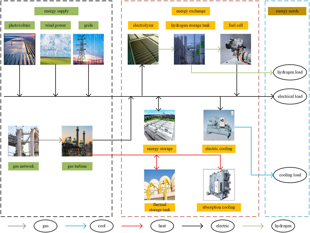
Figure 1. Structure diagram of the integrated energy system of the industrial park.

2.2 Flexible load modeling

2.2.1 Flexible load modeling

Non-interruptible loads (Song et al., 2020) refer to loads that do not respond to real-time prices. Common non-interruptible loads in integrated parks include lighting facilities, heating systems, etc. The mathematical model is as shown in Equations 1, 2 below:

$P^{\text{ul}}\left(t\right)={\gamma }_{\mathrm{e}}^{\text{ul}}\left(t\right)P_0^{\text{de}}\left(t\right)(1)$

$H^{\text{ul}}\left(t\right)={\gamma }_{\mathrm{h}}^{\text{ul}}\left(t\right)H_0^{\text{de}}\left(t\right)(2)$

Where, $P^{\text{ul}}\left(t\right)$、 $H^{\text{ul}}\left(t\right)$ represent the electrical and thermal power demand of non-interruptible loads. ${\gamma }_{\mathrm{e}}^{\text{ul}}\left(t\right)$ and ${\gamma }_{\mathrm{h}}^{\text{ul}}\left(t\right)$ represent the proportion of non-interruptible loads in the total electrical and thermal load demand of the energy hub, and $P_0^{\text{de}}\left(t\right)$ and $H_0^{\text{de}}\left(t\right)$ represent the system’s electrical and thermal load values under the benchmark electricity price.

2.2.2 Transferable load modeling

Transferable loads refer to loads with fixed energy usage time but flexible energy form selection based on needs. Typical transferable loads include air conditioning systems and kitchen equipment based on electrically-driven hybrid cooling. As shown in Equations 3, 4 below:

${\stackrel{\sim }{P}}^{\text{el}}\left(t\right)={\gamma }_{\mathrm{e}}^{\text{el}}\left(t\right)P_0^{\text{de}}\left(t\right)\left[1+\frac{{\stackrel{\sim }{\epsilon }}^{\text{el}}\left(t\right)\left({\rho }^{\mathrm{e}}\left(t\right)-{\rho }^{\mathrm{h}}\left(t\right)\right)}{{\rho }^{\mathrm{h}}\left(t\right)}\right](3)$

${\stackrel{\sim }{H}}^{\text{el}}\left(t\right)={\gamma }_{\mathrm{h}}^{\text{el}}\left(t\right)H_0^{\text{de}}\left(t\right)-{\delta }^{\text{el}}\left[{\stackrel{\sim }{P}}^{\text{el}}\left(t\right)-{\gamma }_{\mathrm{e}}^{\text{el}}\left(t\right)P_0^{\text{de}}\left(t\right)\right](4)$

Where, ${\stackrel{\sim }{P}}^{\text{ts}}\left(t\right)$ represents the electrical load demand of transferable loads under real-time electricity prices, ${\gamma }^{\text{ts}}\left(t\right)$ represents the proportion of transferable loads in the total electrical load demand of the energy hub, ${\rho }^{\mathrm{e}}\left(t\right)$ and ${\rho }_0^{\mathrm{e}}\left(t\right)$ represent the real-time electricity price and the benchmark electricity price, and ${\stackrel{\sim }{\epsilon }}^{\text{ts}}\left(t\right)$, ${\stackrel{\sim }{\epsilon }}^{\text{ts}}\left(t^{\prime }\right)$ represent uncertain variables.

2.2.3 Shiftable load modeling

Shiftable loads refer to loads with a fixed total energy consumption within a certain time period, but with flexible adjustment of the energy usage time. Common shiftable loads in energy systems include water heaters and electric vehicles. In demand response based on real-time electricity prices, users adjust their electricity usage time flexibly according to dynamic changes in electricity prices, which can be expressed by the following price elasticity model as shown in Equation 5 below:

$\begin{array}{l}{\stackrel{\sim }{P}}^{\text{ts}}\left(t\right)={\gamma }^{\text{ts}}\left(t\right)P_0^{de}\left(t\right)\left[1+\frac{{\stackrel{\sim }{\epsilon }}^{\text{ts}}\left(t\right)\left({\rho }^{\mathrm{e}}\left(t\right)-{\rho }_0^{\mathrm{e}}\left(t\right)\right)}{{\rho }_0^{\mathrm{e}}\left(t\right)}\right]+\\ {\displaystyle \sum _{t^{\prime }\in T,t^{\prime }\ne t}} \frac{{\gamma }^{\text{ts}}\left(t^{\prime }\right)P_0^{\text{de}}\left(t^{\prime }\right){\stackrel{\sim }{\epsilon }}^{\text{ts}}\left(t^{\prime }\right)\left({\rho }^{\mathrm{e}}\left(t^{\prime }\right)-{\rho }_0^{\mathrm{e}}\left(t^{\prime }\right)\right)}{{\rho }_0^{\mathrm{e}}\left(t^{\prime }\right)}\end{array}(5)$

Where, ${\stackrel{\sim }{P}}^{\text{ts}}\left(t\right)$ represents the electrical load demand of transferable loads under real-time electricity prices, ${\gamma }^{\text{ts}}\left(t\right)$ represents the proportion of transferable loads in the total electrical load demand of the energy hub, ${\rho }^{\mathrm{e}}\left(t\right)$ and ${\rho }_0^{\mathrm{e}}\left(t\right)$ represent the real-time electricity price and the benchmark electricity price, and ${\stackrel{\sim }{\epsilon }}^{\text{ts}}\left(t\right)$ and ${\stackrel{\sim }{\epsilon }}^{\text{ts}}\left(t^{\prime }\right)$ represent uncertain variables.

2.3 Energy storage system modeling

2.3.1 Electric energy storage modeling

In microgrids that include renewable energy, using batteries to compensate for the differences between energy production and energy demand is one of the most common solutions. The available energy of a battery is typically measured by the “State of Charge” (SOC), and it can be calculated by monitoring the changes in charging power ($P_{\mathrm{B},\text{CH}}$) and discharging power ($P_{\mathrm{B},\text{DIS}}$) over time as shown in Equation 6 below:

$SOC\left(t\right)=SOC\left(t-1\right)+\frac{\left(P_{\mathrm{B},\text{CH}}\cdot {\eta }_{\mathrm{B},\text{CH}}-P_{\mathrm{B},\text{DIS}}/{\eta }_{\mathrm{B},\text{DIS}}\right)\Delta t}{N_{\mathrm{B}}{U}_{\mathrm{B}}{Q}_{\mathrm{B}}}(6)$

2.3.2 Flywheel energy storage modeling

Flywheel energy storage (Ali et al., 2023) is a type of energy storage that converts electrical energy into mechanical energy and vice versa. It uses a rotor to store electrical energy as mechanical energy. During charging, a permanent magnet synchronous motor drives the rotor to rotate and store energy, while during discharging, the flywheel rotor drives the permanent magnet synchronous motor to generate electrical energy. The parameters of a typical flywheel unit are shown in Table 1.

Table 1

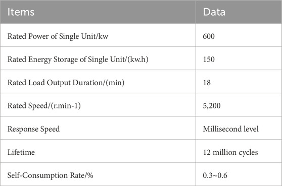
Table 1. Parameters of a flywheel unit.

The amount of energy stored in the flywheel is proportional to the square of its rotational speed, and the energy expression is as shown in Equation 7 below:

$E=\frac{1}{2}J{\omega }^2=\frac{1}{2}J{\left(\frac{2\pi n}{60}\right)}^2=\frac{{\pi }^{2}J}{1800}\times n^2(7)$

Where, $J$ is the polar moment of inertia of the flywheel rotor, measured in $kg·m^2$; $\omega$ is the angular velocity of the flywheel rotor, measured in $rad/s$; and $n$ is the rotational speed of the flywheel rotor, measured in $r/\mathit{min}$.

2.3.3 Thermal energy storage modeling

In integrated energy systems, the thermal energy storage system is often a thermal storage tank. Its mathematical model is as shown in Equation 8 below:

$E_{\mathrm{e}}\left(t\right)=\left(1-{\tau }_{\mathrm{e}}\right)E_{\mathrm{e}}\left(t-1\right)+\left(q_{\text{es}}\left(t\right){\eta }_{\text{es}}+\frac{q_{\text{ed}}\left(t\right)}{{\eta }_{\text{ed}}}\right)\Delta t(8)$

Where, ${\eta }_{\text{es}}$ and ${\eta }_{\text{ed}}$ are the charging and discharging rates of the thermal storage system respectively; $q_{\text{es}}\left(t\right)$ and $q_{\text{ed}}\left(t\right)$ are the charging power and discharging power of the thermal storage system respectively; ${\tau }_{\mathrm{e}}$ is the decay rate; $E_{\mathrm{e}}\left(t\right)$ and $E_{\mathrm{e}}\left(t-1\right)$ are the energy stored at time $t$ and $t-1$ respectively; $\Delta t$ is the unit scheduling time interval.

2.3.4 Cooling energy storage modeling

The general mathematical model for cooling energy storage in the integrated energy system is As shown in Equations 9–13 below:

$S_{\mathrm{s}}^{\text{ch}}\left(t\right)\cdot P_{\mathrm{s},\min }^{\text{ch}}\le P_{\mathrm{s}}^{\text{ch}}\left(t\right)\le S_{\mathrm{s}}^{\text{ch}}\left(t\right)\cdot P_{\mathrm{s},\max }^{\text{ch}}(9)$

$S_{\mathrm{s}}^{\text{dis}}\left(t\right)\cdot P_{\mathrm{s},\min }^{\text{dis}}\le P_{\mathrm{s}}^{\text{dis}}\left(t\right)\le S_{\mathrm{s}}^{\text{dis}}\left(t\right)\cdot P_{\mathrm{s},\min }^{\text{dis}}(10)$

$E_{\mathrm{s}}\left(t\right)=\left(1-{\delta }_{\mathrm{s}}\right)E_{\mathrm{s}}\left(t-1\right)+{\eta }_{\mathrm{s}}^{\text{ch}}{P}_{\mathrm{s}}^{\text{ch}}\left(t-1\right)-\frac{P_{\mathrm{s}}^{\text{dis}}\left(t-1\right)}{{\eta }_{\mathrm{s}}^{\text{dis}}}(11)$

$E_{\mathrm{s},T}=E_{\mathrm{s},0}(12)$

$E_{\mathrm{s},\min }\le E_{\mathrm{s}}\left(t\right)\le E_{\mathrm{s},\max }(13)$

Where, $P_{\mathrm{s}}^{\text{ch}}\left(t\right)$ and $P_{\mathrm{s}}^{\text{dis}}\left(t\right)$ are the generalized expressions for the charging power and discharging power of the cooling energy storage in the integrated energy system; $S_{\mathrm{s}}^{\text{ch}}\left(t\right)$ and $S_{\mathrm{s}}^{\text{dis}}\left(t\right)$ are the charging and discharging states of the cooling energy storage; $P_{\mathrm{s},\min }^{\text{ch}}$, $P_{\mathrm{s},\max }^{\text{ch}}$, $P_{\mathrm{s},\min }^{\text{dis}}$, and $P_{\mathrm{s},\max }^{\text{dis}}$ are the upper and lower limits of the charging power and discharging power of the cooling energy storage in the system; $E_{\mathrm{s}}\left(t\right)$ is the cooling energy storage capacity; ${\delta }_{\mathrm{s}}$ is the self-discharge rate coefficient of the energy storage; ${\eta }_{\mathrm{s}}^{\text{ch}}$ and ${\eta }_{\mathrm{s}}^{\text{dis}}$ are the charging and discharging efficiency coefficients of the cooling energy storage; $E_{\mathrm{s},0}$ and $E_{\mathrm{s},\mathrm{T}}$ are the capacities of the energy storage device at the beginning and end times respectively; $E_{\mathrm{s},\max }$ and $E_{\mathrm{s},\min }$ are the upper and lower limits of the cooling energy storage capacity.

2.4 Hydrogen storage system modeling

2.4.1 Electrolyzer

The electrolyzer (Wang et al., 2023; Dong et al., 2024) is an essential facility for hydrogen production through water electrolysis. In an electrolyzer, water reacts with electricity, producing hydrogen at the cathode and oxygen at the anode. The hydrogen production rate is expressed as shown in Equations 14, 15 below:

${\mathrm{q}}_{\mathrm{H}2}={\eta }_{\mathrm{f}}\frac{{\mathrm{n}}_{\mathrm{c}}{\mathrm{I}}_{\mathrm{E}}}{2\mathrm{F}}(14)$

${\eta }_{\mathrm{f}}=96\mathit{exp}\left(\frac{0.09}{{\mathrm{I}}_{\text{El}}}-\frac{75.5}{{\mathrm{I}}^2\text{El}}\right)(15)$

Where, ${\mathrm{q}}_{\mathrm{H}2}$ is the hydrogen production rate of the electrolyzer; ${\mathrm{n}}_{\mathrm{c}}$ is the number of cells in series; $\mathrm{F}$ is the Faraday constant; ${\mathrm{I}}_{\mathrm{E}}$ is the current; ${\eta }_{\mathrm{f}}$ is the Faraday efficiency. The electricity consumption of the electrolyzer is defined as shown in Equation 16 below:

$P_{\mathrm{E}}=B_{\mathrm{E}}\times H_{\mathrm{N}}+A_{\mathrm{E}}\times H(16)$

Where, $P_{\mathrm{E}}$ is the electricity consumption of the electrolyzer; $H_{\mathrm{N}}$ is the nominal hydrogen production rate of the electrolyzer; $H$ is the actual hydrogen production rate; $A_{\mathrm{E}}$ and $B_{\mathrm{E}}$ are consumption curve coefficients $\left(kWh/kg\right)$.

2.4.2 Fuel cell

Fuel cells (Zheng et al., 2023; Yang et al., 2014) are composed of multiple single cells connected in series. The voltage and power of the fuel cell are calculated using the following equations 17, 18:

$P_{\text{stack}}=n_{\text{cell}}{V}_{\text{cell}}\times Ai(17)$

$V_{\text{stack}}=n_{\text{cell}}{V}_{\text{cell}}(18)$

Where, $V_{\text{cell}}$ is the voltage of a single cell. Due to unavoidable energy losses, the actual operating voltage of the cell is lower than the theoretical voltage. Common losses include activation loss ${\eta }_{\mathrm{a}}$, ohmic loss ${\eta }_{\mathrm{o}}$, and concentration loss ${\eta }_{\mathrm{c}}$. Therefore, the operating voltage is calculated as shown in Equations 19–23 below.

$V_{\text{cell}}=E_{\text{Ne}}-{\eta }_{\mathrm{a}}-{\eta }_{\mathrm{o}}-{\eta }_{\mathrm{c}}(19)$

$\begin{array}{l}{E}_{\text{Ne}}=1.229-\frac{163.23}{2\mathrm{F}}\left(\mathrm{T}-298.15\right)\\ +\frac{\text{RT}}{2\mathrm{F}}\mathit{ln}\left[\frac{p_{{\mathrm{H}}_2}^{\mathrm{m}}}{1.01\times {10}^5}\times {\left(\frac{p_{{\mathrm{O}}_2}^{\mathrm{c}}}{1.01\times {10}^5}\right)}^{0.5}\right]\end{array}(20)$

${\eta }_{\mathrm{a}}=\frac{\text{RT}}{2{\alpha }_{{\mathrm{H}}_2}\mathrm{F}}\mathit{ln}\left(\frac{i+i_{\text{le}}}{i_{{\mathrm{H}}_2}}\right)+\frac{\text{RT}}{4{\alpha }_{{\mathrm{O}}_2}\mathrm{F}}\mathit{ln}\left(\frac{i+i_{\text{le}}}{i_{{\mathrm{O}}_2}}\right)(21)$

${\eta }_{\mathrm{c}}=\frac{\text{RT}}{2\mathrm{F}}\left(1+\frac{1}{c}\right)\times \mathit{ln}\frac{i_1}{i_1-\left(i+i_{\text{le}}\right)}(22)$

${\eta }_{\mathrm{o}}=\frac{i{\delta }_{\mathrm{M}}}{{\alpha }_{\mathrm{c}}\left(0.52\lambda -0.33\right)\mathit{exp}\left[1268\left(\frac{1}{303.15}-\frac{1}{\mathrm{T}}\right)\right]}+i\mathrm{A}{R}_0(23)$

Where, $E_{\text{Ne}}$ is the voltage; $p_{{\mathrm{H}}_2}^{\mathrm{m}}$ is the partial pressure of hydrogen in the anode channel; $p_{{\mathrm{O}}_2}^{\mathrm{c}}$ is the partial pressure of oxygen in the cathode channel. $\mathrm{T}$ is the stack temperature; $\lambda$ is the membrane water content; $i_{\text{le}}$ is the current density loss; $\mathrm{A}$ is the effective area of the cell; ${\delta }_{\mathrm{M}}$ is the thickness of the dry membrane; ${\alpha }_{\mathrm{c}}$ is the conductivity ratio coefficient; $i_{{\mathrm{H}}_2}$ and $i_{{\mathrm{O}}_2}$ are the hydrogen and oxygen exchange current densities respectively; ${\alpha }_{{\mathrm{H}}_2}$ and ${\alpha }_{{\mathrm{O}}_2}$ are the hydrogen and oxygen charge transfer coefficients respectively; $R_0$ is the internal resistance; $\mathrm{F}$ is the Faraday constant; $\mathrm{R}$ is the gas constant.

2.4.3 Methanation reactor

Excess hydrogen is converted into methane through a methanation reactor, providing raw materials for chemical plants or natural gas networks and generating additional revenue. The Power-to-Gas (P2G) process consists of two steps: water electrolysis and methanation. Electrical energy is first converted into hydrogen (H₂) via water electrolysis in the electrolyzer. The hydrogen can either be directly injected into the natural gas network or enter a methanation reactor to react with carbon dioxide (CO₂) to produce methane (CH₄), which is then injected into the natural gas network. The chemical equation for the methanation reaction is as shown in Equation 24 below:

$\begin{array}{l}2{\mathrm{H}}_2\mathrm{O}\to 2{\mathrm{H}}_2+{\mathrm{O}}_2\\ 4{\mathrm{H}}_2+{\text{CO}}_2\to {\text{CH}}_4+2{\mathrm{H}}_2\mathrm{O}\end{array}(24)$

2.4.4 Hydrogen storage tank

In the hydrogen storage system, when the power supplied by renewable energy sources (RES) exceeds demand, the electrolyzer generates hydrogen. The molar flow rate of hydrogen $\left(n_{\text{el}}\right)$ produced by the electrolyzer can be expressed as a function of the supplied power $\left({\mathrm{P}}_{\text{el}}\right)$ as shown in Equation 25 below:

$n_{\text{el}}=\frac{{\eta }_{\text{el}}{\mathrm{P}}_{\text{el}}}{\mathrm{H}}(25)$

Where, $\mathrm{H}$ is the lower heating value of hydrogen (Hui et al., 2022) $\left(240\text{MJ}/\text{kmol}\right)$; ${\eta }_{\text{el}}$ is the efficiency of the electrolyzer. During peak periods, hydrogen can generate electricity through fuel cells. The hydrogen consumption of a fuel cell is related to its power output as shown in Equation 26 below:

$n_{\text{fc}}=\frac{P_{\text{fc}}}{\mathrm{H}}(26)$

Where, $n_{\text{fc}}$ is the efficiency of the fuel cell. $p_{{\mathrm{H}}_2}\left(t\right)$ is the pressure in the hydrogen storage tank at a specific time $t$, an important control variable in the hydrogen storage system. The pressure in the hydrogen storage tank serves as a measure of the hydrogen content in the container and can be expressed using the molar flow rate of hydrogen produced, the molar flow rate of hydrogen consumed, and the pressure $p_{{\mathrm{H}}_2}\left(t-1\right)$ from the previous time step. The specific formula is as shown in Equation 27 below:

$p_{{\mathrm{H}}_2}\left(t\right)=p_{{\mathrm{H}}_2}\left(t-1\right)+\frac{\mathcal{R}{T}_{{\mathrm{H}}_2}}{V_{{\mathrm{H}}_2}}\left(n_{\text{el}}-n_{\text{fc}}\right)(27)$

Where, $\mathcal{R}$ is the gas constant; $T_{{\mathrm{H}}_2}$ is the average temperature inside the container; $V_{{\mathrm{H}}_2}$ is the total volume of the container.

2.5 Gas turbine

A gas turbine is a typical gas-powered generation device that utilizes natural gas for electricity production. The gas turbine model is expressed as shown in Equation 28 below:

$q_g\left(t\right)={\eta }_{\mathrm{t}}{q}_{\mathrm{t}}{\phi }_{\mathrm{g}}(28)$

Where, $q_g\left(t\right)$ represents the electric power output of the gas turbine at time $t$; ${\phi }_{\mathrm{g}}$ denotes the lower heating value of the gas; ${\eta }_{\mathrm{t}}$ represents the gas-to-electric conversion efficiency of the gas turbine; $q_{\mathrm{t}}$ indicates the gas consumption of the gas turbine.

2.6 Electric refrigeration

The mathematical model for electric refrigeration equipment is expressed as shown in Equation 29 below:

$q_{\text{er}}\left(t\right)=q_{\mathrm{c}}\left(t\right){\eta }_{\text{er}}(29)$

Where, $q_{\text{er}}\left(t\right)$ represents the cooling power output of the electric refrigeration power equipment at time $t$; $q_{\mathrm{c}}\left(t\right)$ denotes the electric power consumed by the electric refrigeration equipment at time $t$; ${\eta }_{\text{er}}$ represents the electric-to-cooling power conversion efficiency of the electric refrigeration equipment.

2.7 Electric heating

Electric heating equipment can reduce the heating burden of an integrated energy system by consuming electrical energy to provide users with high-grade thermal energy, offering an additional pathway for renewable energy utilization. Its mathematical model is expressed as shown in Equation 30 below:

$\left\{\begin{array}{l}0⩽P^{\text{eb}}\left(t\right)⩽P_{\max }^{\text{eb}}\\ H^{\text{eb}}\left(t\right)={\mu }_{\text{eb}}{P}^{\text{eb}}\left(t\right)\\ C_{\text{eb}}={\omega }_{\text{eb}}{\displaystyle \sum _{t=1}^{24}} P^{\text{eb}}\left(t\right)\end{array}\right.(30)$

Where, ${\mu }_{\text{eb}}$ represents the electric-to-heat conversion efficiency of the electric heating equipment; $H^{\text{eb}}\left(t\right)$ represents the thermal power of the electric heating equipment at time $t$; $P^{\text{eb}}\left(t\right)$ and $P_{\max }^{\text{eb}}$ represent the power of the electric heating equipment at time $t$ and its maximum value respectively; ${\omega }_{\text{eb}}$ and $C_{\text{eb}}$ represent the electric energy conversion coefficient and cost of the electric heating equipment respectively.

2.8 Absorption refrigeration equipment

The absorption refrigeration plant can be expressed by the following (Equation 31).

$q_{\mathrm{a}}\left(t\right)=q_{\mathrm{h}}\left(t\right){\eta }_{\mathrm{a}}(31)$

Where, $q_{\mathrm{a}}\left(t\right)$ represents the cooling power output of the absorption chiller at time $t$; $q_{\mathrm{h}}\left(t\right)$ represents the thermal power consumed by the absorption chiller at time $t$; ${\eta }_{\mathrm{a}}$ represents the heat-to-cooling conversion efficiency of the absorption chiller.

2.9 Modeling of the uncertainty of wind and photovoltaic power output

2.9.1 Modeling of the uncertainty of wind power output

Wind power generation is closely related to wind speed, which exhibits significant natural variability, making its uncertainty more pronounced. The accuracy of wind power generation predictions is directly affected by how well wind speed is modeled and forecast. In this study, the three-parameter Weibull distribution (de Miguel et al., 2017) is introduced to reduce the error between simulated and actual wind speeds, thereby improving the accuracy of the wind and solar power uncertainty model. Assuming that wind speed follows the three-parameter Weibull distribution, its probability density function can be expressed as shown in Equation 32 below:

$f\left(v\right)=\frac{\beta }{{\eta }^{\beta }}{\left(v-\lambda \right)}^{\left(\beta -1\right)}\exp \left[-{\left(\frac{v-\lambda }{\eta }\right)}^{\beta }\right](32)$

Where, $v$ represents the wind speed; β, η, and $\delta$ represent the shape parameter, scaling parameter, and location parameter respectively. The distribution parameter is given by Equation 33:

$F\left(\nu \right)=1-\exp {\left[-\left(\frac{v-\lambda }{\eta }\right)\right]}^{\beta }(33)$

2.9.2 Modeling of the uncertainty of photovoltaic power output

Photovoltaic power output is significantly influenced by environmental factors, and due to the strong randomness of solar irradiance, it is difficult to accurately describe the solar irradiance. Within a specific time period, solar irradiance approximately follows the Beta distribution (Suresh and Sreejith, 2017). The probability density function of solar irradiance is expressed as shown in Equation 34 below:

$f\left(\frac{G_{\mathrm{T}}}{G_{\text{TS}}}\right)=\frac{\mathrm{\Gamma }\left(\alpha +\delta \right)}{\mathrm{\Gamma }\left(\alpha \right)\mathrm{\Gamma }\left(\delta \right)}{\left(\frac{G_{\mathrm{T}}}{G_{\text{TS}}}\right)}^{\overline{\alpha }-1}{\left(1-\frac{G_{\mathrm{T}}}{G_{\text{TS}}}\right)}^{\delta -1}(34)$

Where, $G_{\text{TS}}$ and $G_{\mathrm{T}}$ represent the incident radiation on the surface under ideal and actual conditions respectively; $\left(•\right)$ represents the Gamma function (Jiao, 2021) , as shown in Equation 35 below:

$\mathrm{\Gamma }\left(\alpha \right)={\int }_0^{\infty } x^{\alpha -1}{e}^{-x}dx(35)$

$\alpha$ and $\delta$ are the shape parameters of the Beta distribution. As shown in Equation 36 below:

$\begin{array}{l}\alpha =\mu \left[\frac{\mu \left(1-\mu \right)}{{\gamma }^2}-1\right]\\ \delta =\left(1-\mu \right)\left[\frac{\mu \left(1-\mu \right)}{{\gamma }^2}-1\right]\end{array}(36)$

Where, $\mu$ and $\gamma$ represent the mean and variance of solar irradiance during the corresponding time period respectively.

2.10 Generation of typical scenarios

2.10.1 Scenario generation based on the Monte Carlo method

The Monte Carlo method is a numerical computational technique based on random sampling and statistical simulation, used to solve complex problems and evaluate system performance (2017). The core idea of this method is to approximate the calculation of target quantities or system characteristics by using a large number of random samples, thereby obtaining an estimate of the solution or performance of the problem. In this section, the Monte Carlo method is used to generate wind-solar scenarios for an entire year. The specific steps are as follows:

Step 1: Obtain the probability distribution model of wind and solar power output.

Step 2: Randomly sample from the model obtained in Step 1.

Step 3: Generate scenarios that satisfy the probability distribution model.

Step 4: Use the wind speed-to-wind power conversion formula to obtain wind power scenarios. The wind speed-to-wind power conversion formula is as shown in Equation 37 below:

$P_{\text{WT},\mathrm{t}}=\left\{\begin{array}{l}\begin{array}{cc}0& {\mathrm{V}}_{\text{WT},\mathrm{t}}<{\mathrm{V}}_{\text{in}}\text{or\hspace{0.5em}}{\mathrm{V}}_{\text{out}}\le {\mathrm{V}}_{\text{WT},\mathrm{t}}\end{array}\\ \begin{array}{cc}\begin{array}{l}\frac{1}{2}\rho {\text{AV}}_{\text{WT},\mathrm{t}}^3{\mathrm{C}}_{\mathrm{P}}\\ P_{\mathrm{N}}\end{array}& \begin{array}{l}{\mathrm{V}}_{\text{in}}\le {\mathrm{V}}_{\text{WT},\mathrm{t}}<{\mathrm{V}}_{\text{rated}}\\ {\mathrm{V}}_{\text{rated}}\le {\mathrm{V}}_{\text{WT},\mathrm{t}}<{\mathrm{V}}_{\text{out}}\end{array}\end{array}\end{array}\right.(37)$

Where, $P_{\text{WT},\mathrm{t}}$ is the output power of the wind turbine at time $t$; $P_{\mathrm{N}}$ is the rated power of the wind turbine; ${\mathrm{V}}_{\text{WT},\mathrm{t}}$ is the wind speed at the hub height of the turbine at time $t$; ${\mathrm{V}}_{\text{rated}}$ is the rated wind speed of the wind turbine; ${\mathrm{V}}_{\text{in}}$ is the wind speed reduction rate of the wind turbine; ${\mathrm{V}}_{\text{out}}$ is the cut-out wind speed of the wind turbine; $\rho$ is the air density; $\mathrm{A}$ is the turbine swept area; ${\mathrm{C}}_{\mathrm{P}}$ is the Betz constant.

Step 5: Use the irradiance-to-power conversion formula to obtain photovoltaic power generation scenarios. The irradiance-to-power conversion formula is as shown in Equation 38 below:

$P_{\text{PV}}=f_{\text{PV}}\left(\frac{G_{\mathrm{T}}}{G_{\text{TS}}}\right)\left[1+\mu \left(-T_{\text{CS}}\right)\right](38)$

Where, $Y_{\text{PV}}$ represents the nominal capacity of the photovoltaic cell; $G_{\text{TS}}$ and $G_{\mathrm{T}}$ represent the incident radiation on the surface under ideal and actual conditions respectively; $\mu$ represents the temperature coefficient of the conversion efficiency; $T_{\text{CS}}$ and $T_{\mathrm{C}}$ represent the surface temperature of the battery under standard and actual conditions respectively. The temperature calculation for the time step is as shown in Equation 39 below:

$T_{\mathrm{c}}=\left(\frac{T_{\mathrm{a}}+\left(-T_{\text{an}}\right)\left(\frac{G_{\mathrm{T}}}{G_{\text{TS}}}\right)\left(\frac{\left[1-{\eta }_{\text{AS}}\left(1-\mu \cdot T_{\text{CS}}\right)\right]}{a}\right)}{1+\left(T_{\text{cn}}-T_{\text{an}}\right)\left(\frac{G_{\mathrm{T}}}{G_{\text{TS}}}\right)\left(\frac{{\mu }_{\mathrm{a}}{\eta }_{\text{AS}}}{a}\right)}\right)(39)$

Where, $T_{\text{an}}$ and $T_{\text{cn}}$ represent the surface temperature of the battery under nominal and actual conditions respectively; ${\eta }_{\text{AS}}$ represents the solar system efficiency under maximum power conditions; $a$ is the temperature parameter.

2.10.2 K-means clustering for scenario reduction

K-means clustering (Vardakas and Likas, 2024) is a commonly used unsupervised learning algorithm for dividing a dataset into k distinct groups. The core idea of the algorithm is to iteratively assign data points to the nearest cluster center and update the cluster centers to minimize the squared error within the clusters. In this section, this method is used to reduce the wind-solar scenarios from the previous section. The specific steps are as follows:

Step 1: Select k scenarios as the initial cluster centers.

Step 2: Calculate the distance between each scenario and the cluster centers, and assign each scenario to the nearest cluster center, thus forming k clusters.

Step 3: For each cluster, calculate the average of its member scenarios and use this average as the new cluster center.

Step 4: Repeat Steps 2 and 3 until the maximum number of iterations is reached or the cluster centers no longer change.

Step 5: Count the number of scenarios in each cluster, normalize, and use it as the probability of selecting that cluster center.

Step 6: Based on the final scenario probabilities, randomly select the corresponding scenarios to complete the scenario reduction. The specific flow chart for generating wind-solar uncertainty scenarios is shown in Figure 2.

Figure 2

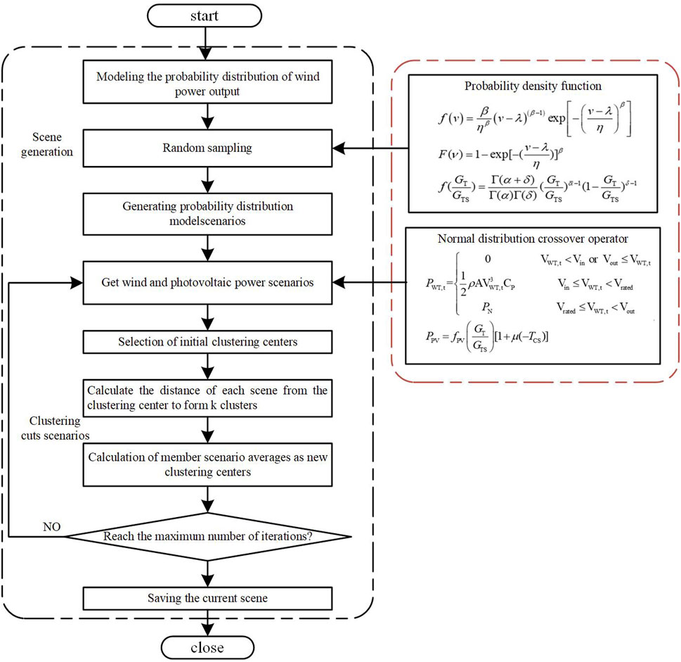
Figure 2. Flow chart of K-means clustering algorithm.

3 Bi-level planning configuration and scheduling optimization model

In this study, the planning and scheduling models are tightly coupled and interact with each other to jointly optimize the system’s operation and configuration. The planning model optimizes the configuration of energy storage, electrical, and thermal equipment, determines the system’s installed capacity and costs, and provides equipment capacity and operational constraints for the scheduling model. The scheduling model, based on the planning results, schedules equipment (such as wind power, photovoltaic power, energy storage, etc.) to maximize operational revenue, balancing energy sales, purchases, operation and maintenance, subsidies, and environmental costs. Conversely, the scheduling results feed back into the planning process. If phenomena such as curtailment of wind or solar energy occur, the planning model will be prompted to adjust the system configuration to reduce waste and optimize costs. Therefore, the planning and scheduling models achieve overall system optimization through a dynamic feedback mechanism.

3.1 Planning objective function

Considering the costs associated with wind and solar curtailment, the following planning configuration objective function is designed, as shown in Equations 40–43 below:

$c_{\text{total}}=\min \left(c_1+c_2+c_3\right)(40)$

Where, $c_1$ represents the operating cost of the energy storage system; $c_2$ represents the generation cost of the generator units; $c_3$ represents the penalty cost for wind and solar curtailment.

$c_1=k{u}_{\mathrm{P}}{\displaystyle \sum _{i\in \phi }}{u}_i^{\mathrm{P}}+k{u}_{\text{CHP}}{\displaystyle \sum _{i\in \phi }}{u}_i^{\text{CHP}}+k{u}_{\text{GF}}{\displaystyle \sum _{i\in \phi }}{u}_i^{\text{GF}}+k{u}_{\text{EV}}{\displaystyle \sum _{i\in \phi }}{u}_i^{\text{EV}}(41)$

$c_2={\displaystyle \sum _{i\in S_{\mathrm{G}}}}\left({\alpha }_i+{\beta }_i{P}_{\mathrm{G}i}+{\delta }_i{P}_{\mathrm{G}i}^2\right)(42)$

$c_3=p_{\text{penal}.\mathrm{l}}{\displaystyle \sum _{t=1}^T}{L}_{\text{des}.t}+p_{\text{penal}.2}{\displaystyle \sum _{t=1}^T}{L}_{\text{loss}.t}(43)$

Where, $k$ is the annualized investment coefficient; $\phi$ represents the total number of energy stations in the area; $u_i^{\mathrm{P}}$, $u_i^{\text{CHP}}$, $u_i^{\text{GF}}$ and $u_i^{\text{EV}}$ represent the total capacity of the grid, CHP system, wind power and photovoltaic power systems in the park respectively; $u_{\mathrm{P}}$, $u_{\text{CHP}}$, $u_{\text{GF}}$ and $u_{\text{EV}}$ represent the unit construction costs; ${\alpha }_i$, ${\beta }_i$ and ${\delta }_i$ are the cost coefficients of generation fuel; $P_{\mathrm{G}i}$ represents the active power of the generator; $p_{\text{penal}.\mathrm{l}}$ represents the penalty price per unit of curtailed wind and solar energy; $p_{\text{penal}.2}$ represents the penalty price per unit of lost regional load; $L_{\text{des}.t}$ represents the amount of curtailed wind and solar energy; $L_{\text{loss}.t}$ represents the amount of load lost due to insufficient spinning reserve of the system; $T$ represents the total operation time of scheduling.

3.2 Scheduling objective function

This study aims to maximize the system’s operational revenue, and its objective function is mathematically expressed as shown in Equations 44–48 below:

$\max f_1=R_{\mathrm{e}}-C_{\mathrm{e}}-C_{\mathrm{o}}-C_{\mathrm{d}}-C_{\mathrm{p}}(44)$

Where, $R_{\mathrm{e}}$ represents the system’s energy sales revenue; $C_{\mathrm{e}}$ represents the energy purchase cost; $C_{\mathrm{o}}$ represents the operation and maintenance costs of various equipment; $C_{\mathrm{d}}$ represents the subsidy cost; $C_{\mathrm{p}}$ represents the environmental cost.

$\begin{array}{l}{R}_{\mathrm{e}}={\displaystyle \sum _{t=1}^{T_1}}{p}_{\mathrm{e}}^{\mathrm{s}}\left(t\right)\left({\stackrel{\sim }{q}}_{\mathrm{e}}\left(t\right)+q_{\mathrm{e}}^{\mathrm{i}}\left(t\right)-q_{\mathrm{e}}^{\mathrm{o}}\left(t\right)\right)+{\displaystyle \sum _{t=1}^{T_1}}{p}_{\mathrm{h}}^{\mathrm{s}}\left(t\right){\stackrel{\sim }{q}}_{\mathrm{h}}\left(t\right)+{\displaystyle \sum _{t=1}^{T_1}}{p}_{\mathrm{c}}^{\mathrm{s}}\left(t\right){\stackrel{\sim }{q}}_{\mathrm{c}}\left(t\right)\end{array}(45)$

$C_{\mathrm{o}}={\displaystyle \sum _{t=1}^{T_1}}\left(\begin{array}{l}{c}_{\mathrm{w}}{q}_{\mathrm{w}}\left(t\right)+c_{\mathrm{e}}{q}_{\mathrm{e}}\left(t\right)+c_{\mathrm{a}}{q}_{\mathrm{a}}\left(t\right)+c_{\text{wt}}{q}_{\text{wt}}\left(t\right)\\ +c_{\text{pv}}{q}_{\text{pv}}\left(t\right)+c_{\text{es}}\left(q_{\text{ch}}^{\text{es}}\left(t\right)+q_{\text{di}}^{\text{es}}\left(t\right)\right)\\ +c_{\text{te}}\left(q_{\text{ch}}^{\text{te}}\left(t\right)+q_{\text{di}}^{\text{te}}\left(t\right)\right)+c_{\mathrm{f}}{q}_{\mathrm{f}}\left(t\right)\end{array}\right)(46)$

$C_{\mathrm{d}}={\displaystyle \sum _{t=1}^{T_1}}{c}_{\mathrm{d}}{q}_{\mathrm{e}}^{\mathrm{o}}\left(t\right)(47)$

$C_{\mathrm{p}}={\displaystyle \sum _{t=1}^{T_1}}\left(c_{\mathrm{t}}{q}_{\mathrm{t}}\left(t\right)+c_{\mathrm{r}}{q}_{\mathrm{r}}\left(t\right)\right)(48)$

Where, $T_1$ represents the scheduling period in the day-ahead stage; $p_{\mathrm{e}}^{\mathrm{s}}\left(t\right)$, $p_{\mathrm{h}}^{\mathrm{s}}\left(t\right)$ and $p_{\mathrm{c}}^{\mathrm{s}}\left(t\right)$ represent the sales prices of electricity, heat, and cooling at time $t$ respectively; ${\stackrel{\sim }{q}}_{\mathrm{e}}\left(t\right)$, ${\stackrel{\sim }{q}}_{\mathrm{h}}\left(t\right)$ and ${\stackrel{\sim }{q}}_{\mathrm{c}}\left(t\right)$ represent the fuzzy parameters of electrical load, thermal load, and cooling load at time $t$ respectively; $q_{\mathrm{e}}^{\mathrm{i}}\left(t\right)$ and $q_{\mathrm{e}}^{\mathrm{o}}\left(t\right)$ represent the amount of electricity load shifted in and out of the system at time $t$ respectively; $p_{\mathrm{e}}^{\mathrm{b}}\left(t\right)$ represents the electricity purchase price from the grid at time $t$; $q_{\mathrm{e}}^{\mathrm{b}}\left(t\right)$ represents the electricity purchased at time $t$; $p_{\mathrm{g}}^{\mathrm{b}}$ represents the natural gas purchase price; $q^g\left(t\right)$ represents the natural gas purchase volume at time $t$; $c_{\mathrm{w}}$, $c_{\mathrm{e}}$, $c_{\mathrm{a}}$, $c_{\text{wt}}$, $c_{\text{pv}}$, $c_{\text{es}}$, $c_{\text{te}}$ and $c_{\mathrm{f}}$ represent the operation and maintenance costs of equipment power for gas turbines, electric chillers, absorption chillers, wind power units, photovoltaic units, energy storage systems, thermal storage systems and other system equipment, respectively; $q_{\mathrm{w}}\left(t\right)$, $q_{\mathrm{e}}\left(t\right)$, $q_{\mathrm{a}}\left(t\right)$ , $q_{\text{wt}}\left(t\right)$, $q_{\text{pv}}\left(t\right)$ and $q_{\mathrm{f}}\left(t\right)$ represent the equipment power of gas turbines, electric cooling systems, absorption cooling systems, wind power units, photovoltaic units and other system equipment, respectively; $q_{\text{ch}}^{\text{es}}\left(t\right)$ and $q_{\text{di}}^{\text{es}}\left(t\right)$ represent the charging power and discharging power of the energy storage system respectively; $q_{\text{ch}}^{\text{te}}\left(t\right)$ and $q_{\text{di}}^{\text{te}}\left(t\right)$ represent the storage power and release power of the thermal storage system respectively; $c_{\mathrm{d}}$ represents the subsidies provided by the system to users; $c_{\mathrm{t}}$ and $c_{\mathrm{r}}$ represent the pollutant emission cost of gas turbines and the cost of curtailed wind and photovoltaic power respectively; $q_{\mathrm{w}}\left(t\right)$ and $q_{\mathrm{r}}\left(t\right)$ represent the output power of gas turbines and curtailed renewable energy at time $t$ , respectively.

3.3 Constraint conditions

3.3.1 Power balance constraint

As shown in Equation 49 below is power balance constraint.

$Cr\{{\stackrel{\sim }{q}}_{\text{wt}}+{\stackrel{\sim }{q}}_{\text{pv}}+q_g\left(t\right)+q_{\text{di}}^{\text{es}}\left(t\right)+q_{\mathrm{e}}^{\mathrm{b}}\left(t\right)+q_{\mathrm{e}}^{\mathrm{o}}\left(t\right)=q_{\text{ch}}^{\text{es}}\left(t\right)+{\stackrel{\sim }{q}}_t^{\mathrm{s}}+q_{\mathrm{e}}^i\left(t\right)\}\ge {\alpha }_{\mathrm{p}}(49)$

Where, $Cr\left\{·\right\}$ represents the probability of event occurring in $\left\{·\right\}$; ${\stackrel{\sim }{q}}_{\text{wt}}$ and ${\stackrel{\sim }{q}}_{\text{pv}}$ represent the fuzzy parameters of wind and photovoltaic power output at time $t$ , respectively.

3.3.2 Equipment power constraints

Equipment constraints include output constraints and ramp rate constraints as shown in Equations 50, 51 below:

$0\le q_{\mathrm{m}}\left(t\right)\le q_{\mathrm{m}}^{\max }(50)$

$\left|q_{\mathrm{m}}\left(t+1\right)-q_{\mathrm{m}}\left(t\right)\right|\le q_{\mathrm{m},\mathrm{r}}^{\max }\cdot \Delta t(51)$

Where, $q_{\mathrm{m}}\left(t\right)$ represents the output power of equipment $\mathrm{m}$ at time; $q_{\mathrm{m}}^{\max }$ represents the upper power limit of the corresponding equipment; $q_{\mathrm{m},\mathrm{r}}^{\max }$ represents the ramp-up rate.

3.3.3 Electricity purchase constraint

As shown in Equation 52 below is electricity purchase constraint.

$0\le q_{\mathrm{e}}^{\mathrm{b}}\left(t\right)\le q_{\max }^{\text{grid}}(52)$

Where, $q_{\max }^{\text{grid}}$ represents the upper power limit of electric energy.

3.3.4 Energy storage constraint

As shown in Equations 53–56 below are energy storage constraint.

$0\cdot {\lambda }_{\text{ch}}^{\text{es}}\left(t\right)\le q_{\text{ch}}^{\text{es}}\left(t\right)\le q_{\max }^{\text{es}}{\lambda }_{\text{ch}}^{\text{es}}\left(t\right)(53)$

$0\cdot {\lambda }_{\text{di}}^{\text{es}}\left(t\right)\le q_{\text{di}}^{\text{es}}\left(t\right)\le q_{\max }^{\text{es}}{\lambda }_{\text{di}}^{\text{es}}\left(t\right)(54)$

$SO{C}_{\min }\le SOC\left(t\right)\le SO{C}_{\max }(55)$

${\lambda }_{\text{ch}}^{\text{es}}\left(t\right)+{\lambda }_{\text{di}}^{\text{es}}\left(t\right)\le 1(56)$

Where, $q_{\max }^{\text{es}}$ represents the upper power limit for charging and discharging energy; ${\lambda }_{\text{ch}}^{\text{es}}\left(t\right)$ and ${\lambda }_{\text{di}}^{\text{es}}\left(t\right)$ represent the maximum and minimum states of charge for the energy storage system; $SOC\left(t\right)$ represents the stored electric energy; $SO{C}_{\max }$ and $SO{C}_{\min }$ represent the maximum and minimum storage energy levels of the energy storage system, respectively.

3.3.5 Cost constraint

To prevent direct transactions with the grid, the cost of purchasing energy from the integrated energy system should not exceed the cost of purchasing energy directly from an energy supplier. The cost constraint is expressed as shown in Equations 57, 58 below:

$\begin{array}{l}{\displaystyle \sum _{t=1}^{T_1}}\left[\begin{array}{l}{p}_{\mathrm{e}}^{\mathrm{s}}\left(t\right)\left({\stackrel{\sim }{q}}_{\mathrm{e}}\left(t\right)+q_{\mathrm{e}}^{\mathrm{i}}\left(t\right)-q_{\mathrm{e}}^{\mathrm{o}}\left(t\right)\right)+\\ p_{\mathrm{h}}^{\mathrm{s}}\left(t\right){\stackrel{\sim }{q}}_{\mathrm{h}}\left(t\right)+p_{\mathrm{c}}^{\mathrm{s}}\left(t\right){\stackrel{\sim }{q}}_{\mathrm{c}}\left(t\right)\end{array}\right]\\ \le {\displaystyle \sum _{t=1}^{T_1}}\left[\begin{array}{l}{p}_{\mathrm{e}}^{\mathrm{b}}\left(t\right)\left({\stackrel{\sim }{q}}_{\mathrm{e}}\left(t\right)+q_{\mathrm{e}}^{\mathrm{i}}\left(t\right)-q_{\mathrm{e}}^{\mathrm{o}}\left(t\right)\right)+\\ p_{\mathrm{h}}^{\mathrm{b}}\left(t\right){\stackrel{\sim }{q}}_{\mathrm{h}}\left(t\right)+p_{\mathrm{c}}^{\mathrm{b}}\left(t\right){\stackrel{\sim }{q}}_{\mathrm{c}}\left(t\right)\end{array}\right]\end{array}(57)$

$0\le c_t^{\text{dr}}\le c_{\max }^{\text{dr}}(58)$

Where, $p_{\mathrm{h}}^{\mathrm{b}}\left(t\right)$ represents the heating price of the heating network at time $t$; $c_{\max }^{\text{dr}}$ represents the maximum subsidy price for demand response.

3.3.6 Demand constraint

The load shifting at time $t$ in the integrated energy system must satisfy its upper and lower limits, as shown in Equations 59–61 below:

$0\le q_{\mathrm{e}}^{\mathrm{o}}\left(t\right),q_{\mathrm{e}}^{\mathrm{i}}\left(t\right)\le {\mu }_{\max }^{\mathrm{l}}\left(t\right){\stackrel{\sim }{q}}_{\mathrm{e}}\left(t\right)(59)$

${\displaystyle \sum _{t=1}^{T_1}}{q}_{\mathrm{e}}^{\mathrm{o}}\left(t\right)={\displaystyle \sum _{t=1}^{T_1}}{q}_{\mathrm{e}}^{\mathrm{i}}\left(t\right)(60)$

$q_{\mathrm{e}}^{\mathrm{o}}\left(t\right)\cdot q_{\mathrm{e}}^{\mathrm{i}}\left(t\right)=0(61)$

Where, ${\mu }_{\max }^{\mathrm{l}}\left(t\right)$ represents the percentage of load shifted at time t.

3.3.7 Fuzzy constraints

Electric Power Balance Constraint as shown in Equation 62 below:

$\begin{array}{l}\left(2-2{\alpha }_{\mathrm{p}}\right)\left[{\stackrel{\sim }{q}}_{\mathrm{e}}^3\left(t\right)-{\stackrel{\sim }{q}}_{\mathrm{w}}^2\left(t\right)-{\stackrel{\sim }{q}}_{\mathrm{s}}^2\left(t\right)\right]+-q_{\mathrm{e}}^{\mathrm{b}}\left(t\right)\\ \left(2{\alpha }_{\mathrm{p}}-1\right)\left[{\stackrel{\sim }{q}}_{\mathrm{e}}^4\left(t\right)-{\stackrel{\sim }{q}}_{\mathrm{w}}^1\left(t\right)-{\stackrel{\sim }{q}}_{\mathrm{s}}^1\left(t\right)\right]+q_{\mathrm{e}}^{\mathrm{i}}\left(t\right)\\ +q_{\text{ch}}^{\text{es}}\left(t\right)-q_{\text{di}}^{\text{es}}\left(t\right)-q_g\left(t\right)-q_{\mathrm{e}}^{\mathrm{o}}\left(t\right)=0\end{array}(62)$

Thermal Power Balance Constraint as shown in Equation 63 below:

$\left(2-2{\alpha }_{\mathrm{p}}\right){\stackrel{\sim }{q}}_{\mathrm{h}}^3\left(t\right)+\left(2{\alpha }_{\mathrm{p}}-1\right){\stackrel{\sim }{q}}_{\mathrm{h}}^4\left(t\right)+q_{\mathrm{a}}\left(t\right)+q_{\text{ch}}^{\text{te}}\left(t\right)-q_{\text{di}}^{\text{te}}\left(t\right)=0(63)$

Cooling Power Balance Constraint as shown in Equation 64 below:

$\left(2-2{\alpha }_{\mathfrak{p}}\right){\stackrel{\sim }{q}}_{\mathfrak{c}}^3\left(t\right)-q_{\mathfrak{e}\mathfrak{r}}\left(t\right)+\left(2{\alpha }_{\mathfrak{p}}-1\right){\stackrel{\sim }{q}}_{\mathfrak{c}}^4\left(t\right)-q_{\mathfrak{a}}\left(t\right)=0(64)$

Where, ${\stackrel{\sim }{q}}_{\mathrm{e}}^3\left(t\right)$, ${\stackrel{\sim }{q}}_{\mathrm{e}}^4\left(t\right)$, ${\stackrel{\sim }{q}}_{\mathrm{h}}^3\left(t\right)$, ${\stackrel{\sim }{q}}_{\mathrm{h}}^4\left(t\right)$, ${\stackrel{\sim }{q}}_{\mathrm{c}}^3\left(t\right)$ and ${\stackrel{\sim }{q}}_{\mathrm{c}}^3\left(t\right)$ represent the membership parameters for the predicted values of electrical load, thermal load, and cooling load; ${\stackrel{\sim }{q}}_{\mathrm{w}}^2\left(t\right)$, ${\stackrel{\sim }{q}}_{\mathrm{w}}^1\left(t\right)$, ${\stackrel{\sim }{q}}_{\mathrm{s}}^2\left(t\right)$ and ${\stackrel{\sim }{q}}_{\mathrm{s}}^2\left(t\right)$ represent the membership parameters for the predicted outputs of wind and solar power.

3.3.8 Carbon emission cost function

The primary goal of our study is to optimize the configuration and scheduling of an integrated energy system (IES) in a low-carbon city while minimizing operational costs and reducing carbon emissions. The optimization objective function should explicitly account for carbon emission costs as part of the overall operational expenses. To address this, we have re-examined the formulation of the objective function and ensured that it incorporates all relevant cost components, including:

1) Energy procurement costs: costs associated with purchasing electricity, natural gas, or other fuels.renewable

2) Energy curtailment costs: losses incurred due to the inability to fully utilize wind and solar power.

3) Carbon emission costs: costs associated with greenhouse gas emissions, which are typically quantified using a carbon tax or cap-and-trade mechanism.

4) Hydrogen production and storage costs: Expenses related to producing and storing hydrogen for energy storage and backup generation.

The revised objective function can be expressed as shown in Equation 65 below:

$C_{total}=C_{energy}+C_{curtailment}+C_{carbon}+C_{hydrogen}(65)$

Where, $C_{energy}$ represents the cost of procuring energy from external sources. $C_{curtailment}$ represents the cost of curtailing renewable energy output. $C_{carbon}$ represents the cost of carbon emissions, calculated as the product of emission rates and a carbon price. $C_{hydrogen}$ represents the cost of hydrogen production and storage. This value was used to calculate the carbon emission costs for each scenario. Emission factors for different energy sources were derived from standard databases, such as 0.82 kg CO₂/kWh for coal-fired electricity and 0.18 kg CO₂/kWh for natural gas-fired electricity.

4 Enhanced Kepler Optimization Algorithm

4.1 Traditional kepler algorithm

The Kepler Optimization Algorithm (Von Loeper et al., 2020; Abdel-Basset et al., 2023) is a novel physics-based metaheuristic algorithm inspired by Kepler’s laws of planetary motion, which can predict the position and velocity of planets at any given time. In the Kepler Optimization Algorithm, each planet and its position represent a candidate solution, which is randomly updated during the optimization process. The computational steps of the Kepler Optimization Algorithm are as follows:

Step 1: Initialization

In this initialization step, N planets are randomly distributed within a d-dimensional search space. Each planet represents a potential solution, corresponding to the decision variables of the optimization problem. The initialization process is governed by the following (Equation 66):

$\begin{array}{l}{X}_i^j=X_{i,\text{low}}^j+\mathit{ran}{d}_{\left[0,1\right]}\times \left(X_{i,\text{up}}^j-X_{i,\text{low}}^j\right)\\ i=1,2,\dots ,\mathrm{N};j=1,2,\dots ,\mathrm{d}\end{array}(66)$

Where, $X_i^j$ represents the j-th decision variable of the i-th planet (candidate solution) in the search space; $\mathrm{N}$ represents the number of candidate solutions in the search space; d represents the dimension of the problem to be optimized; $X_{i,\text{up}}^j$ and $X_{i,\text{low}}^j$ represent the upper and lower bounds of the j-th decision variable respectively; $\mathit{ran}{d}_{\left[0,1\right]}$ is a random number generated between 0 and 1. The orbital eccentricity $e_i$ of the i-th object is initialized using the following (Equation 67):

$e_i=\mathit{ran}{d}_{\left[0,1\right]},i=1,\dots ,\mathrm{N}(67)$

Where, $\mathit{ran}{d}_{\left[0,1\right]}$ is a random value generated within the interval [0,1]. The orbital period of the i-th object is initialized using the following (Equation 68):

$T_i=\left|r\right|,i=1,\dots ,\mathrm{N}(68)$

Where, $r$ represents the number randomly generated based on a normal distribution.

Step 2: Define Gravity

Gravity is the fundamental force controlling the motion of planets around the sun. Each planet exerts its own gravitational force, which is proportional to its mass. The closer a planet is to the sun, the higher its orbital velocity, and vice versa. The gravitational attraction between the sun $X_{\mathrm{s}}$ and any planet $X_{\mathrm{i}}$ is defined by Newton’s law of universal gravitation as shown in Equation 69 below:

$F_{\text{gi}}\left(t\right)=e_{\mathrm{i}}\times \mu \left(t\right)\times \frac{{\overline{M}}_{\mathrm{s}}\times {\overline{m}}_{\mathrm{i}}}{{\overline{R}}_{\mathrm{i}}^2+\epsilon }+r_1(69)$

Where, ${\overline{M}}_{\mathrm{s}}$ and ${\overline{m}}_{\mathrm{i}}$ represent the normalized values of $M_{\mathrm{s}}$ and $m_{\mathrm{i}}$, corresponding to the masses of $X_{\mathrm{s}}$ and $X_{\mathrm{i}}$; $\mu$ represents the gravitational constant; $e_{\mathrm{i}}$ represents the orbital eccentricity of the planet, a value between 0 and 1; $r_1$ is a random value generated between 0 and 1; ${\overline{R}}_{\mathrm{i}}$ represents the Euclidean distance between $X_{\mathrm{s}}$ and $X_{\mathrm{i}}$.

Step 3: Calculate the Velocity of Objects

The velocity of an object depends on its position relative to the sun. The velocity of an object orbiting the sun can be calculated using the following (Equation 70):

$V_i\left(t\right)=\left\{\begin{array}{l}\mathcal{l}\times \left(2r_4{\overrightarrow{X}}_i-{\overrightarrow{X}}_b\right)+\mathcal{l}\times \left({\overrightarrow{X}}_a-{\overrightarrow{X}}_b\right)+\left(1-R_{i-norm}\left(t\right)\right)\\ \times \mathcal{F}\times {\overrightarrow{U}}_1\times {\overrightarrow{r}}_5\times \left({\overrightarrow{X}}_{i,up}-{\overrightarrow{X}}_{i,low}\right),\text{if}{R}_{i-norm}\left(t\right)\le 0.5\\ r_4\times \mathcal{L}\times \left({\overrightarrow{X}}_a-{\overrightarrow{X}}_i\right)+\left(1-R_{i-norm}\left(t\right)\right)\times \mathcal{F}\times U_2\times {\overrightarrow{r}}_5\\ \times \left(r_3{\overrightarrow{X}}_{i,up}-{\overrightarrow{X}}_{i,low}\right),\text{if}{R}_{i-norm}\left(t\right)>0.5\end{array}\right.(70)$

Where, $V_i\left(t\right)$ represents the velocity of object $i$ at time $t$; ${\overrightarrow{X}}_i$ represents object $i$; $r_3$ and $r_4$ are random values generated within the interval [0,1]; ${\overrightarrow{r}}_5$ is a random vector between 0 and 1. ${\overrightarrow{X}}_a$ and ${\overrightarrow{X}}_b$ represent selected solutions.

Step 4: Escape from Local Optima

In the solar system, most celestial bodies rotate counterclockwise; however, some celestial bodies orbit the sun in a clockwise direction. KOA leverages this behavior to escape local optima and simulates this behavior by changing the search direction flag F, allowing a broader scan of the search space.

Step 5: Update Object Position

Celestial bodies revolve around the sun in their own elliptical orbits. During their rotation, objects move closer to the sun for a period and then move away. This behavior is simulated in the algorithm through two main phases: the exploration phase and the exploitation phase. The mathematical expression is given as:

$\begin{array}{l}{\overrightarrow{X}}_i\left(t+1\right)={\overrightarrow{X}}_i\left(t\right)+\mathcal{F}\times {\overrightarrow{V}}_i\left(t\right)+\\ \left({\mathbf{F}}_{{\mathbf{g}}_i}\left(t\right)+\left|r\right|\right)\times \overrightarrow{U}\times \left({\overrightarrow{X}}_{\mathrm{S}}\left(t\right)-{\overrightarrow{X}}_{\mathrm{i}}\left(t\right)\right)\end{array}(71)$

Where, ${\overrightarrow{X}}_i\left(t+1\right)$ represents the new position of object $i$ at time $t+1$; ${\overrightarrow{V}}_i\left(t\right)$ represents the velocity required for object $i$ to reach the new position; ${\overrightarrow{X}}_{\mathrm{S}}\left(t\right)$ is the best position of the sun discovered so far; $\mathcal{F}$ serves as a flag for changing the search direction.

Step 6: Update the Relative Distance to the Sun

When a planet approaches the sun, KOA focuses on optimizing exploitation operations; when the sun is farther away, KOA prioritizes exploration operations. These behaviors are influenced by the adjustment parameter $\mathrm{h}$, which changes gradually over time. When $\mathrm{h}$ is large, the exploration operator is used to expand the distance between the planetary orbit and the sun. Conversely, when $\mathrm{h}$ is small, the exploitation operator is applied to refine the search in the current area. This step is randomly interchanged with Step 5. The mathematical principle of this step is expressed as shown in Equations 72–74 below:

$\begin{array}{ll}\hfill & \hfill {\overrightarrow{X}}_i\left(t+1\right)={\overrightarrow{X}}_i\left(t\right)\times {\overrightarrow{U}}_1+\left(1-{\overrightarrow{U}}_1\right)\\ \hfill & \hfill \times \left(\frac{{\overrightarrow{X}}_i\left(t\right)+{\overrightarrow{X}}_{\mathrm{S}}+{\overrightarrow{X}}_a\left(t\right)}{3.0}+\mathrm{h}\times \left(\frac{{\overrightarrow{X}}_i\left(t\right)+{\overrightarrow{X}}_{\mathrm{S}}+{\overrightarrow{X}}_a\left(t\right)}{3.0}-{\overrightarrow{X}}_b\left(t\right)\right)\right)\end{array}(72)$

Where, $h$ is an adaptive factor controlling the distance between the sun and the current planet at time. It is defined as:

$h=\frac{1}{e^{\eta r}}(73)$

Where, $r$ is a random number generated based on a normal distribution; $\eta$ is a linearly decreasing factor ranging from $-1$ to $-2$. It is defined as:

$\eta =\left(a_2-1\right)\times r_4+1(74)$

Where, $a_2$ is a cycle control parameter.

Step 7: Obtain the Optimal Solution

This step can be understood simply as an elitist selection strategy. The process is mathematically represented as shown in Equation 75 below:

${\overrightarrow{X}}_{i,new}\left(t+1\right)=\left\{\begin{array}{l}\begin{array}{ccc}{\overrightarrow{X}}_i\left(t+1\right)& ,if& f\left({\overrightarrow{X}}_i\left(t+1\right)\right)\le f\left({\overrightarrow{X}}_i\left(t\right)\right)\end{array}\\ \begin{array}{ccc}{\overrightarrow{X}}_i\left(t\right)& ,if& f\left({\overrightarrow{X}}_i\left(t+1\right)\right)>f\left({\overrightarrow{X}}_i\left(t\right)\right)\end{array}\end{array}\right.(75)$

4.2 Enhanced Kepler Optimization Algorithm

4.2.1 Chaotic mapping strategy

The initialization state of the algorithm determines the convergence speed to some extent. To ensure that planetary individuals are evenly distributed along their orbits, this section introduces a chaotic mapping strategy to optimize the initialization process described in Step 1 of Section 3.1. The enhanced formula is as shown in Equation 76 below:

$X_i^j=\cos \left\{i{\cos }^{-1}\left(X_{i,\text{low}}^j\right)\right\}+\hspace{0.17em}\mathit{ran}{d}_{\left[0,1\right]}\times \left(X_{i,\text{up}}^j-X_{i,\text{low}}^j\right)(76)$

4.2.2 Adaptive learning rate strategy

In the current algorithm, the flag $\mathcal{F}$ is introduced in Step 3 to escape local optima. However, activating this flag from the beginning of the algorithm is not realistic. The issue of escaping local optima typically occurs in the later stages of optimization. At the beginning of the optimization, this strategy should be minimized to improve the efficiency of the optimization process. Therefore, an adaptive learning rate is introduced in this study to reduce changes in flag $\mathcal{F}$ during the early iterations and increase them in the later iterations. The mathematical expression of the adaptive learning rate designed in this paper is as shown in Equation 77 below:

$\eta =\left\{\begin{array}{l}\left(\eta -{\eta }_E\right)\cdot e^{-k\cdot floor\left(V/R\right)}+{\eta }_E,rand\ge p\\ \left(\eta -{\eta }_E\right)\cdot e^{-k\cdot floor\left(V/R\right)}+{\left(\frac{V}{R}\right)}^{0.7}\cdot {\eta }_E,rand<p\end{array}\right.(77)$

Where, ${\eta }_E$ represents the final learning rate from the last iteration; $k$ is the variation factor; $V$ is the number of iterations; $R$ represents the mutation interval; $floor$ is the quotient function; $p$ is the mutation probability term. The flag $\mathcal{F}$ is defined as shown in Equation 78 below:

$\mathcal{F}=\left\{\begin{array}{l}\mathcal{F}\begin{array}{cc}& if\left(p_1\le \eta \right)\end{array}\\ -\mathcal{F}\begin{array}{cc}& if\left(p_1>\eta \right)\end{array}\end{array}\right.(78)$

Where, $p_1$ represents the mutation probability. It can be seen that the adaptive learning factor $\eta$ decreases as the number of iterations increases, while the algorithm’s ability to escape local optima increases with more iterations. This strategy not only enhances the algorithm’s ability to escape local optima but also avoids unnecessary computational power in the early stages of iteration.

4.2.3 Adaptive adjustment parameter

As previously described in Step 6 of Section 3.1, the adjustment parameter $\mathrm{h}$ greatly influences the algorithm’s exploration and exploitation balance. In the original algorithm, the adjustment parameter $\mathrm{h}$ changes randomly. While this randomness enhances the algorithm’s global search capability, it also reduces its optimization efficiency. To balance the algorithm’s efficiency and performance, this section introduces an adaptive adjustment parameter $\mathrm{h}$ that decreases progressively with the number of iterations. In the early iterations, the algorithm focuses on global exploration, while in the later iterations, it concentrates on local exploitation. The mathematical expression for the designed adjustment parameter $\mathrm{h}$ is as shown in Equation 79 below:

$h=\left\{\begin{array}{l}\begin{array}{cc}\frac{1}{e^{\eta r}}.\left(\frac{q_{\max }-q}{q_{\max }}\right)& if\left(h<h^{\prime }\right)\end{array}\\ \begin{array}{cc}{h}^{\prime }& if\left(h\ge h^{\prime }\right)\end{array}\end{array}\right.(79)$

Where, $h$ is the current adjustment parameter; $h^{\prime }$ is the previous adjustment parameter; $q_{\max }$ is the maximum number of iterations; and $q$ is the current number of iterations. The flow chart of the enhanced Kepler Optimization Algorithm is shown in Figure 3.

Figure 3

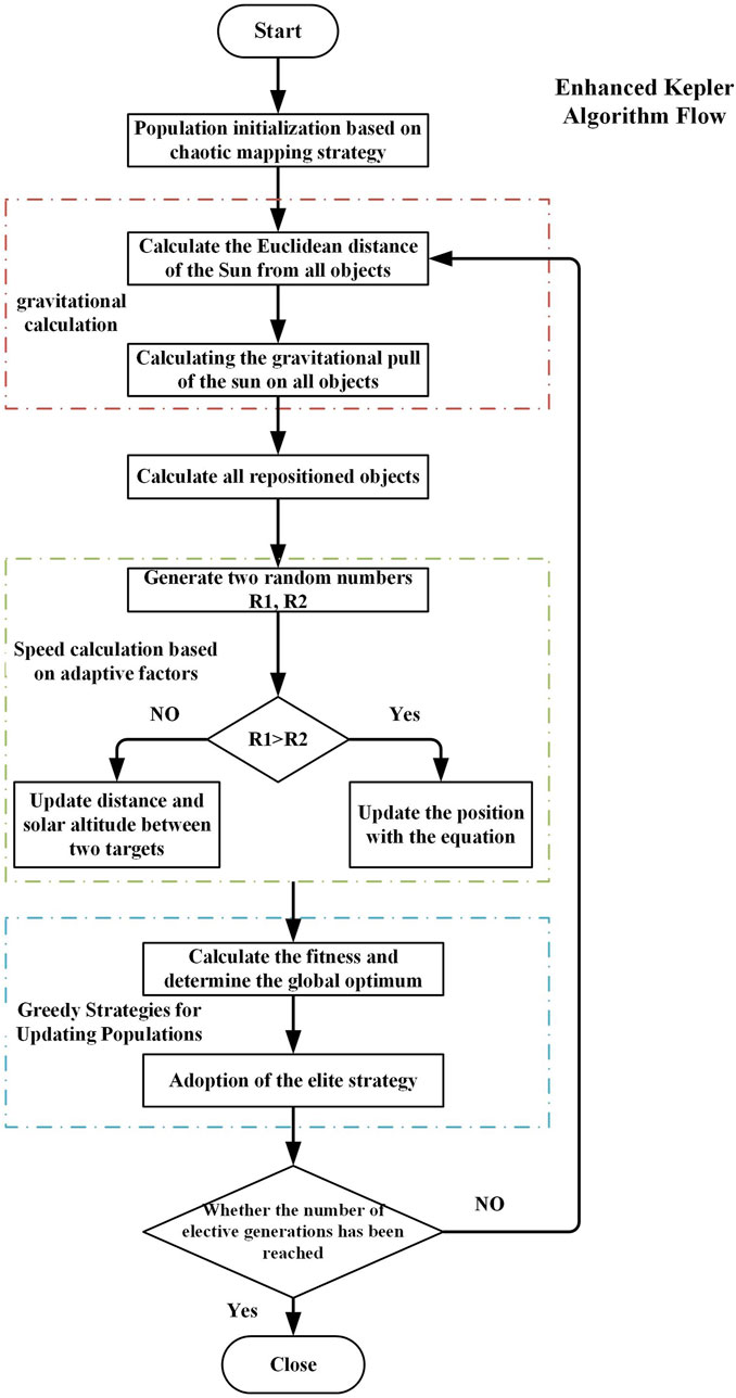
Figure 3. Flow chart of the enhanced Kepler optimization algorithm.

4.3 Algorithm performance verification

To verify the performance of the enhanced Kepler Optimization Algorithm proposed in this paper, tests were conducted using the 3rd, 5th, 13th, and 15th test functions from the CEC2017 benchmark function set. The graphical representations of these test functions are shown in Figure 4.

Figure 4

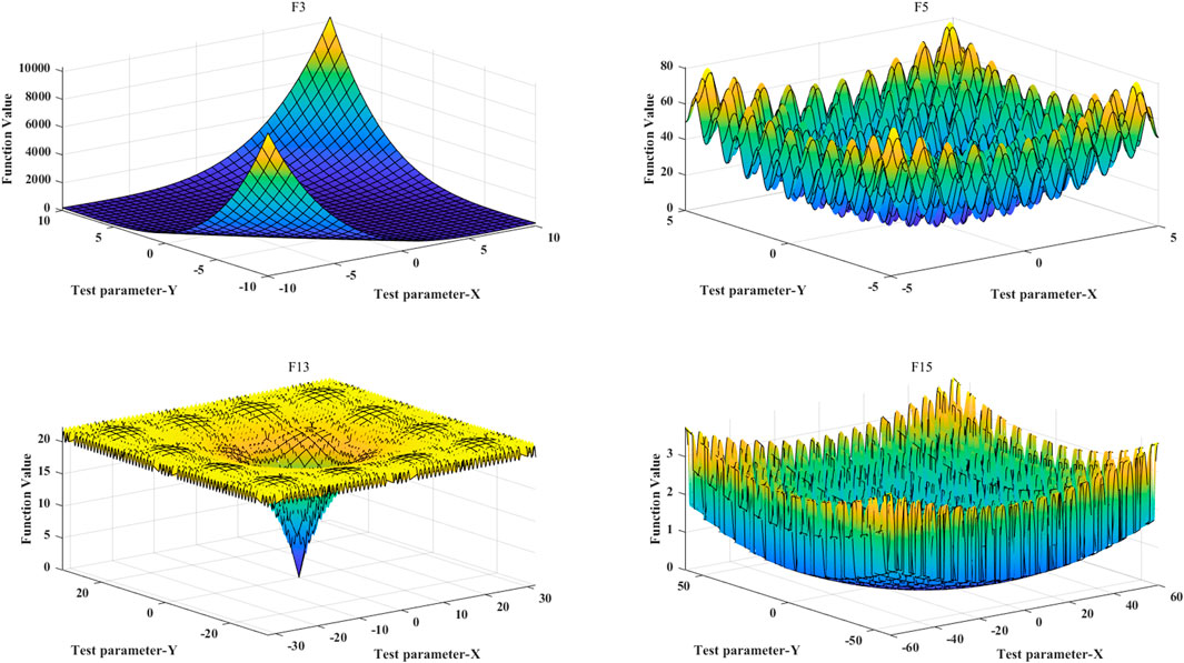
Figure 4. Images of test functions.

Based on the above test functions, the enhanced Kepler Optimization Algorithm proposed in this paper was used to compute the extreme values of the test functions. The enhanced Kepler algorithm was compared with the traditional Kepler algorithm, the Dung Beetle Optimization Algorithm (Jiachen and Li-hui, 2024), and the Starling Algorithm (Cai et al., 2021). The initial conditions for all four algorithms were the same, with a population size of 100 and 100 iterations. The simulation environment for the above algorithms was MATLAB 2022b, running on a computer with an Intel Core i9-13900K processor, 64 GB 3200 MHz RAM, and an RTX 4060 GPU. The final optimization iteration curves are shown in Figure 5.

Figure 5

Figure 5. Iterative convergence curves of the four algorithms.

From Figure 5, it can be seen that the enhanced Kepler algorithm proposed in this paper outperforms the other three traditional methods in terms of convergence speed and computational accuracy. To more clearly demonstrate the effectiveness of the proposed method, the optimization process was repeated 100 times, and the mean, variance, optimal value, and average runtime of all optimization results were calculated. The statistical results are shown in Table 2.

Table 2

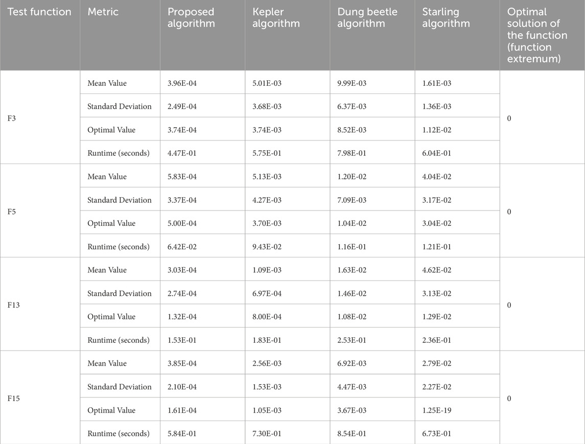
Table 2. Final results of the 100 iterations.

Based on Table 2, it can be observed that the proposed method in this paper outperforms the other three algorithms in all four evaluation metrics: mean, standard deviation, optimal value, and runtime, demonstrating the superiority of the proposed method in performance. Specifically, in terms of the mean value of the F3 test function, the proposed method achieved 3.96E-04, significantly lower than the other algorithms’ 5.01E-03, 9.99E-03, and 1.61E-03. For the optimal value of the F5 test function, the proposed method achieved 5.00E-04, which is also lower than the other algorithms’ 3.70E-03, 1.04E-02, and 3.04E-02. This indicates that the proposed method has higher computational accuracy. In terms of standard deviation, for example, on the F13 test function, the standard deviation of the proposed method was 2.74E-04, much lower than the other algorithms’ 6.97E-04, 1.46E-02, and 3.13E-02, indicating better stability. Regarding runtime, for example, on the F15 test function, the proposed method’s runtime was 5.84E-01 s, clearly faster than the other algorithms’ 7.30E-01 s, 8.54E-01 s, and 6.73E-01 s, improving computational efficiency by approximately 28.8%. In summary, the method proposed in this paper demonstrates better search capabilities and can achieve efficient model solving.

5 Simulation example

In the simulation analysis, the proposed enhanced Kepler algorithm was used to solve the planning configuration and scheduling model. In the planning phase, the objective variable is the total system cost, and the decision variables include the capacities of energy storage, wind power, and photovoltaic power. In the scheduling phase, the objective variable is the total operational income, and the decision variables include energy procurement, power load, natural gas procurement, equipment power, as well as the charging power and discharging power of the energy storage system.

5.1 Basic data

This section conducts a simulation analysis based on the operational data of an industrial park-level integrated energy system in a coastal area of southeastern China. The electricity price is a time-of-use pricing model, and the natural gas price is fixed. The energy price variation curve is shown in Figure 6A, and the load variation curve is shown in Figure 6B. From this figure, it can be seen that the thermal load of the industrial park shows little variation throughout the day, while the cooling load exhibits a pattern of being small at night and large at noon. The electrical load has a distinct pattern of being high during the day and low at night, and the natural gas load shows a significant increase during meal times.

Figure 6

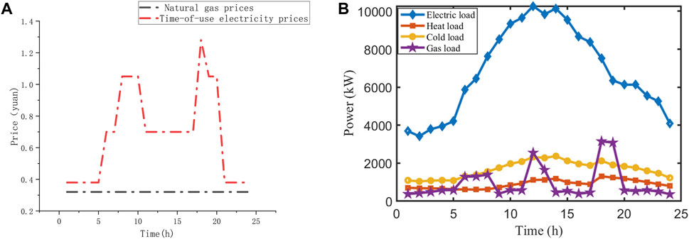
Figure 6. (A) Energy price curve; (B) Cooling, heating and· electrical load curves.

Based on the local meteorological data, typical wind and solar power output scenarios were generated using the typical scenario generation method proposed in this paper, as shown in Figure 7. The scenario reduction method was then applied to reduce the scenarios, resulting in six typical wind power scenarios with probabilities of 0.1, 0.15, 0.1, 0.2, 0.2, and 0.25, and six typical photovoltaic power output scenarios with probabilities of 0.15, 0.25, 0.15, 0.2, 0.05, and 0.2. The final scenarios are shown in Figure 8. The stochastic optimization theory used in the subsequent analysis optimizes the system’s capacity and operating conditions, and therefore, the final wind and solar scenarios used are the expected values of the scenarios shown in Figure 8.

Figure 7

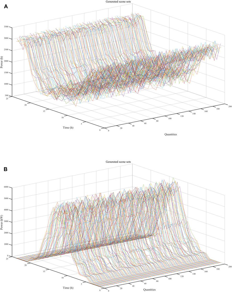
Figure 7. (A) Total wind power scenarios; (B) Total solar power scenarios.

Figure 8

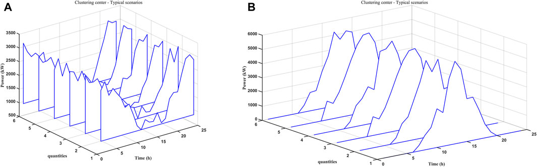
Figure 8. (A) Six typical wind power scenarios; (B) Six typical solar power scenarios.

5.2 Analysis of system configuration results

This section is based on the integrated energy system constructed in Figure 1. It is assumed that no new conventional units such as gas generators and gas boilers will be added, and the capacity of distributed wind-solar renewable energy units and energy storage devices will be configured. Based on the wind-solar power output curves and data of typical load curves from Section 4.1, the economic investment coefficients and capacity limits of each device are shown in Table 3, with other system parameters referenced from reference [26]. The system operation conditions are divided into three types, as shown in Table 4. The final system configuration is presented in Table 5. For ease of calculation, this paper ignores equipment depreciation, adopts integer values for the configuration, and uses 100 kW as the base for variation. Additionally, the capacity of hydrogen storage facilities is represented in KWh, which refers to the total electricity generated when the hydrogen stored in the hydrogen storage tanks is fully used for power generation. It is also assumed that the equipment operates steadily throughout the system’s operating cycle.

Table 3

Table 3. Economic parameters and capacity limits of equipment.

Table 4

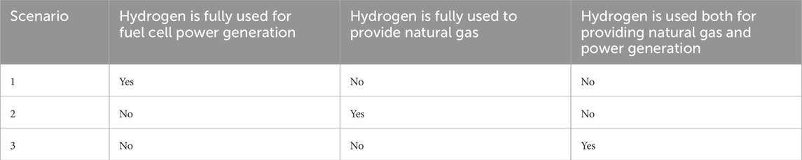
Table 4. Three system operation scenarios.

Table 5

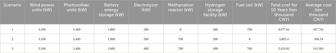
Table 5. Final system configuration.

From the tables above, it can be seen that the configuration of wind and solar units remains the same in all scenarios. This configuration is unrelated to the hydrogen energy’s operation mode and is only dependent on the local wind and solar resource endowment and whether excess electricity is fed back into the grid. In the integrated energy system simulated in this paper, the capacity of wind, solar, and other new energy sources is relatively small, and excess electricity is not fed into the grid. The penalty price for wind and solar curtailment is low. Therefore, the capacity of wind and solar units depends solely on the local wind and solar resource endowment. If the penalty price for wind and solar curtailment is higher, the configuration of wind and solar units will change, with a reduction in the capacity of new energy units. Moreover, the capacity configuration will be negatively correlated with the penalty price.

5.3 Analysis of scheduling optimization results

In the three scenarios mentioned above, the penalty price for wind and solar curtailment is set at 50% of the time-of-use electricity price. The scheduling optimization is then performed for each scenario, and the final operation results are shown in Figure 9. The detailed statistical data of each optimized scenario are presented in Table 6.

Figure 9

Figure 9. (A) scheduling result of scenario 1; (B) scheduling result of scenario 2; (C) scheduling result of scenario 3; (D) cost of scenario 1; (E) cost of scenario 2; (F) cost of scenario 3.

Table 6

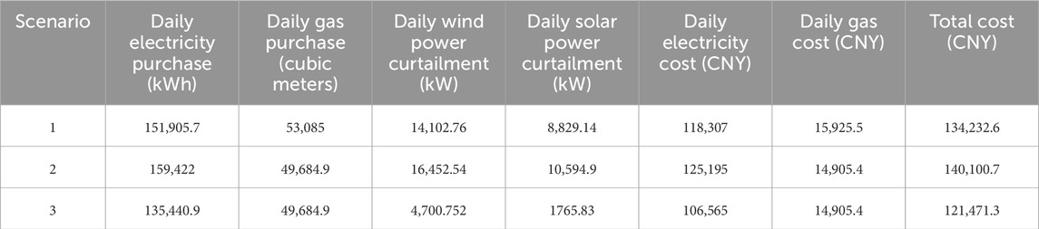
Table 6. Cost statistics of different scenarios.

Qualitative analysis of Figure 9 reveals that Scenario 3 has the best operational economy, with the lowest wind and solar curtailment rates and the least external electricity and gas purchases. Quantitative analysis of Table 6 shows that, compared to Scenario 1, Scenario three reduces the daily electricity purchase by 16,464.8 kWh, and the daily gas purchase by 3,400.1 cubic meters, resulting in a 10.5% reduction in daily costs. Compared to Scenario 2, Scenario three reduces the daily electricity purchase by 23,981.1 kWh, leading to a 15.34% reduction in daily costs. In summary, the investment construction costs of the three scenarios, ranked from lowest to highest, are Scenario 1, Scenario 2, and Scenario 3. When ranked by operating costs, the order from lowest to highest is Scenario 3, Scenario 2, and Scenario 1. Assuming a 10-year investment period, Scenario 3 has a total investment of nearly 5 million yuan higher than Scenario 1, but the annual operating cost of Scenario three is about 4.66 million yuan less than Scenario 1. From this comparison, it can be seen that when the investment payback period exceeds 2 years, the configuration in Scenario three is the most cost-effective. When the payback period is less than 2 years, the configuration in Scenario 1 is more cost-effective, and Scenario 2 is the least economical. This is because the domestic natural gas price is relatively low and stable, and in Scenario 2, the cost of natural gas produced by the methanation reactor is higher than the cost of purchasing gas, making Scenario 2 the least economical.

5.4 Typical seasonal characteristics and validity analysis of different arithmetic examples

In order to be able to reflect the scheduling results in different phases and different periods, we have considered the optimal scheduling under different seasonal characteristics in a year, which is divided into the summer energy consumption process and the winter energy consumption process, and optimized scheduling is carried out based on the different load demands of different energy consumption seasonal characteristics. Based on 2 years of winter and summer data, we obtain the typical winter and summer energy use characteristics in the region, and simulation analysis based on this data, the relevant winter and summer load characteristics obtained are as shown in Figure 10 below.

Figure 10

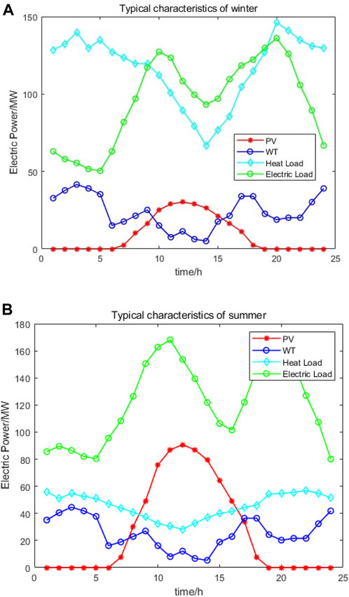
Figure 10. (A) The winter load characteristics; (B) The summer load characteristics.

It is shown that there is a clear load difference characteristic between winter and summer, with higher thermal loads in winter and somewhat higher PV outputs in summer. Based on this typical load characteristics, the results after optimal scheduling using the algorithm in this paper are as shown in Figures 11, 12 below:

Figure 11

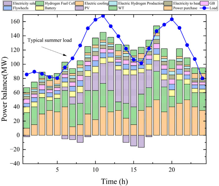
Figure 11. Dispatch results for typical summer character days.

Figure 12

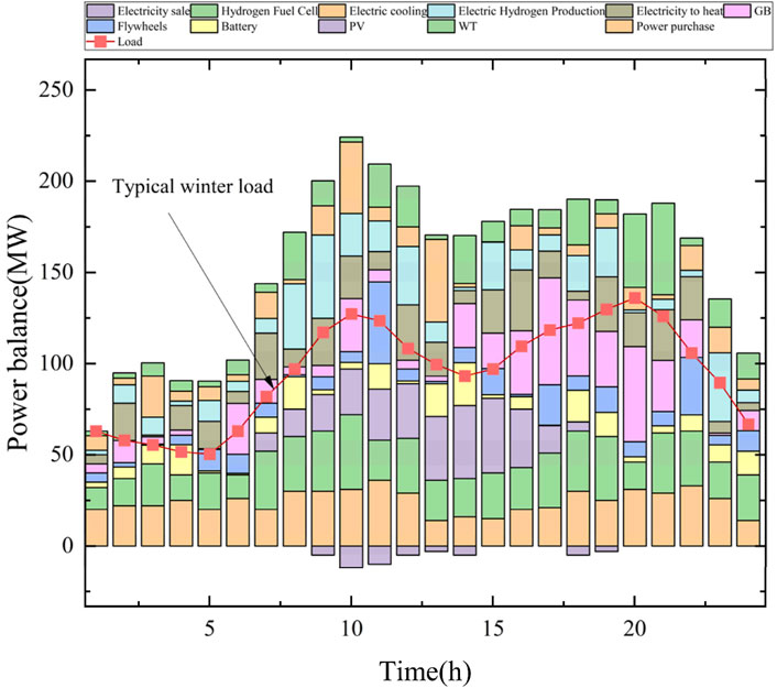
Figure 12. Dispatch results for typical winter character days.

From the distribution pattern of loads, it can be seen that there is a clear seasonal difference between winter and summer, which is reflected in the fact that the overall electricity demand in summer is higher than that in winter, and due to the access of air-conditioning and industrial loads, the overall electricity load in summer is higher than that in winter, and at the same time, the renewable energy output in summer is higher than that in winter, which is particularly obvious in the photovoltaic output, based on the algorithm in this paper, when there is new energy consumption, it will be prioritized Based on the algorithm of this paper, when there is new energy consumption, it will prioritize the new energy consumption, which further saves the carbon cost and improves the consumption of wind and solar power.

To test the convergence performance of the proposed algorithm in different scales, we have chosen two typical scenarios, namely, the improved 32-node thermal system-33-node electric system and the relatively small-scale 6-node thermal system-7-node gas system-14-node electric system, to test whether the algorithm is able to solve the optimal solution and whether it can converge normally, and the corresponding convergence time. optimal solution, and whether it can converge normally, and the corresponding convergence time. The results are shown in Figure 13 below:

Figure 13

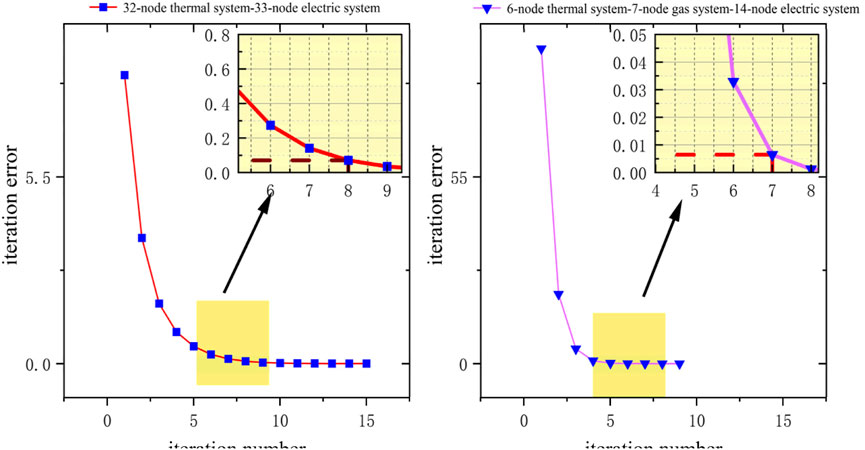
Figure 13. The convergence iteration error of the algorithm for different cases.

It can be seen that the algorithm proposed in this paper is able to converge the iteration error to a reasonable threshold in a limited number of iterations for different scales, which indicates that the algorithm has a certain degree of universality.

Comprehensive the above content, this paper in the following aspects of the content can provide a certain reference value for the relevant engineering applications:

1. For renewable energy modeling: for the uncertainty of wind and solar energy output in the actual operation process, a three-parameter Weibull distribution model (Weibull distribution) and a beta distribution model (Beta distribution) are used to describe it. Compared with the traditional two-parameter Weibull distribution model, our method can more accurately reflect the change patterns of actual wind speed and light intensity. This improvement provides more reliable input data for subsequent dispatch optimization.

2. For terms of load modeling: Based on the above research, we classify flexible loads into three types and combine them with different electricity consumption patterns to achieve the effect of peak shaving and valley filling. This classification method not only helps to reduce the peak-to-valley difference of the system, but also improves the utilization of renewable energy. In industrial scenarios, certain production processes can be adjusted to better match the new energy generation curve by adjusting the running time, thus reducing the phenomenon of wind and light abandonment.

3. For terms of solving algorithm: In order to overcome the deficiencies of traditional optimization algorithms in solving complex scheduling problems, we propose an Enhanced Kepler Optimization Algorithm (EKOA) based on chaotic mapping and adaptive learning rate strategy. The following are the main features of the algorithm and its practical value in engineering applications mainly in the following aspects: accuracy and solution efficiency: EKOA significantly expands the search range of the algorithm and avoids the problem of locally optimal solutions by introducing the chaotic mapping mechanism. This is particularly important for solving high-dimensional optimization problems, especially when multiple variables are involved in an integrated energy system. By dynamically adjusting the learning rate parameter, EKOA is able to accelerate the convergence speed while ensuring accuracy. This enables the algorithm to respond quickly to real-time scheduling demands and is suitable for dynamically changing power system environments. We have verified the role of EKOA in reducing the operating cost of the system and significantly reducing the curtailment rate of wind and photovoltaic power to improve the overall economy in a real case study of an industrial park along the southeast coast. A comparative analysis of different scenarios (Scenario 1, Scenario 2 and Scenario 3) reveals the optimal configuration under different payback cycles.

6 Conclusion

This paper aims to maximize energy utilization efficiency and minimize environmental carbon emissions in industrial parks, involving both system modeling and optimization algorithms. The study focuses on the configuration and scheduling optimization of integrated energy systems with flexible loads, and draws the following conclusions.

(1) This paper employs the three-parameter Weibull distribution model and the Beta distribution model to better describe the uncertainty of wind and solar power output. By categorizing flexible loads into three types and accounting for their distinct electricity consumption patterns, peak shaving and valley filling are achieved, reducing the peak-to-valley difference of the system and thereby increasing the proportion of renewable energy utilization.

(2) An enhanced Kepler algorithm is proposed, incorporating chaotic mapping and adaptive learning rate strategies. Compared to traditional algorithms, the proposed algorithm offers a broader search range, faster convergence speed, and higher solution efficiency, achieving an efficient solution of the integrated energy system’s planning and scheduling models.

(3) The paper proposes an optimal scheduling and configuration method for integrated energy systems and validates the optimization process through a case study of an industrial park’s integrated energy system in the southeastern coastal area. The results show that the proposed method effectively achieves peak shaving and valley filling, reduces wind and solar power curtailment rates, and yields good economic benefits.

It should be noted that this paper only considers hydrogen energy power generation as a single usage path and does not account for the economic benefits of hydrogen sales in the hydrogen energy market. Future research will further incorporate hydrogen energy demand-side response and optimize the integrated energy system’s output from the perspective of the spot market.

Data availability statement

The raw data supporting the conclusions of this article will be made available by the authors, without undue reservation.

Author contributions

ZW: Data curation, Formal Analysis, Investigation, Methodology, Writing–original draft. SW: Investigation, Methodology, Writing–review and editing. HN: Data curation, Formal Analysis, Project administration, Writing–original draft, Writing–review and editing. JW: Data curation, Project administration, Writing–review and editing. JZ: Conceptualization, Data curation, Writing–review and editing.

Funding

The author(s) declare that financial support was received for the research, authorship, and/or publication of this article. This work was supported by National Natural Science Foundation of China (5157147); Open Research Fund Project of Hubei Transmission Line Engineering Technology Research Center (Three Gorges University) (2022KXL03); Research on key technologies and applications of non-stop operation of distribution network transformers (B311JH230001).

Acknowledgments

I would like to express my gratitude to the Open Research Fund Project of Hubei Transmission Line Engineering Technology Research Center (Three Gorges University) (2022KXL03) for their financial support in this research.

Conflict of interest

Author SW was employed by State Grid Zhejiang Wuyi County Power Supply Co., Ltd.

The remaining authors declare that the research was conducted in the absence of any commercial or financial relationships that could be construed as a potential conflict of interest.

Generative AI statement

The author(s) declare that no Generative AI was used in the creation of this manuscript.

Publisher’s note

All claims expressed in this article are solely those of the authors and do not necessarily represent those of their affiliated organizations, or those of the publisher, the editors and the reviewers. Any product that may be evaluated in this article, or claim that may be made by its manufacturer, is not guaranteed or endorsed by the publisher.

References

Abdel-Basset, M., Mohamed, R., Azeem, S. A. A., Jameel, M., and Abouhawwash, M. (2023). Kepler optimization algorithm: a new metaheuristic algorithm inspired by Kepler’s laws of planetary motion. Knowledge-based Syst. 268, 110454. doi:10.1016/j.knosys.2023.110454

CrossRef Full Text | Google Scholar

Akgül, F. G., Şenoğlu, B., and Arslan, T. (2016). An alternative distribution to Weibull for modeling the wind speed data: inverse Weibull distribution. Energy Convers. Manag. 114, 234–240. doi:10.1016/j.enconman.2016.02.026

CrossRef Full Text | Google Scholar

Ali, G., Khosro, D., Jalil, S., Mahdavinejad, M., and Yeganeh, M. (2023). A designerly approach to daylight efficiency of central light-well; combining manual with NSGA-II algorithm optimization. Energy 276(1), 127402. doi:10.1016/j.energy.2023.127402

CrossRef Full Text | Google Scholar

Author anonymous. (2017). Multilevel American Monte Carlo and operational procedures of multilevel Monte Carlo method.

Google Scholar

Cai, S., Qi, L., and Yibin, Q. (2021). Economic evaluation of whole life cycle of the micro-grid system under the mode of residual power connection/hydrogen production. Power Syst. Technol. 45(12), 4650–4660.doi:10.13335/j.1000-3673.pst.2021.0090

CrossRef Full Text | Google Scholar

de Miguel, N., Acosta, B., Moretto, P., Briottet, L., Bortot, P., and Mecozzi, E. (2017). Hydrogen enhanced fatigue in full scale metallic vessel tests–Results from the MATHRYCE project. Int. J. hydrogen energy 42 (19), 13777–13788. doi:10.1016/j.ijhydene.2017.01.144

CrossRef Full Text | Google Scholar

Dong, Y., Ma, Z., Wang, Q., Ma, S., and Han, Z. (2024). Optimal capacity configuration of hybrid electrolytic cells power to hydrogen (P2H) system in distribution system. IEEE Trans. Appl. Supercond. 34, 1–5. doi:10.1109/tasc.2024.3450860

CrossRef Full Text | Google Scholar

Han, Z., Han, W., Ye, Y., and Sui, J. (2024). Multi-objective sustainability optimization of a solar-based integrated energy system. Renew. Sustain. Energy Rev. 202, 114679. doi:10.1016/j.rser.2024.114679

CrossRef Full Text | Google Scholar

Hui, D., Ge, W., Zhang, S., Liu, C., and Chu, C. (2022). Summary of differences between hydrogen production from offshore wind power and direct outward transmission of electric energy. Power Gener. Technol. 43 (6), 869. doi:10.12096/j.2096-4528.pgt.22095

CrossRef Full Text | Google Scholar

Jiachen, H., and Li-hui, F. (2024). Robot path planning based on improved dung beetle optimizer algorithm. J. Braz. Soc. Mech. Sci. Eng. 46 (4), 235. doi:10.1007/s40430-024-04768-3

CrossRef Full Text | Google Scholar

Jiang, J., Zhang, H., and Guo, J. (2024). Short-term wind power prediction based on improved dung beetle optimization algorithm. J. Zhengzhou Univ. Sci., 1–8. doi:10.13705/j.issn.1671-6833.2025.01.015

CrossRef Full Text | Google Scholar

Jiao, M. (2021). Research on simulation analysis of hydrogen leakage and diffusion in hydrogen supply system of fuel cell truck. Beijing: Beijing Jiaotong University.

Google Scholar

Peng, B., Li, Y., Liu, H., Kang, P., Bai, Y., Zhao, J., et al. (2024). Design of energy management strategy for integrated energy system including multi-component electric–thermal–hydrogen energy storage. Energies 17 (23), 6184. doi:10.3390/en17236184

CrossRef Full Text | Google Scholar

Song, Z., Liu, T., and Lin, Q. (2020). Multi-objective optimization of a solar hybrid CCHP system based on different operation modes. Energy 206, 118125. doi:10.1016/j.energy.2020.118125

CrossRef Full Text | Google Scholar

Suresh, V., and Sreejith, S. (2017). Generation dispatch of combined solar thermal systems using dragonfly algorithm. Computing 99 (1), 59–80. doi:10.1007/s00607-016-0514-9

CrossRef Full Text | Google Scholar

Vardakas, G., and Likas, A. (2024). Global k-means++: an effective relaxation of the global k-means clustering algorithm. Appl. Intell. 54 (19), 8876–8888. doi:10.1007/s10489-024-05636-2

CrossRef Full Text | Google Scholar

Von Loeper, F., Schaumann, P., De Langlard, M., Hess, R., Bäsmann, R., and Schmidt, V. (2020). Probabilistic prediction of solar power supply to distribution networks, using forecasts of global horizontal irradiation. Sol. Energy 203, 145–156. doi:10.1016/j.solener.2020.04.001

CrossRef Full Text | Google Scholar

Wang, Y., Song, M., Jia, M., Li, B., Fei, H., Zhang, Y., et al. (2023). Multi-objective distributionally robust optimization for hydrogen-involved total renewable energy CCHP planning under source-load uncertainties. Appl. Energy 342, 121212. doi:10.1016/j.apenergy.2023.121212

CrossRef Full Text | Google Scholar

Xue, J., Wang, D., Yu, Z., Li, H., Zhu, X., and Dou, C. (2019). Joint optimal scheduling of wind and solar diesel storage based on wind power adjustable uncertainty cost. J. Zhengzhou Univ. Sci. 40 (05), 73–79. doi:10.13705/j.issn.1671-6833.2019.05.006

CrossRef Full Text | Google Scholar

Yang, S., Liu, J., Yao, J., Ding, H., Wang, K., and Li, Y. (2014). Model and strategy for multi-time scale coordinated flexible load interactive scheduling. Proc. CSEE 34 (22), 3664–3673. doi:10.13334/j.0258-8013.pcsee.2014.22.011

CrossRef Full Text | Google Scholar

Yang, W., Lin, L., and Gao, H. (2022). Simulation evaluation of small samples based on grey estimation and improved bootstrap. Grey Syst. Theory Appl. 12 (2), 376–388. doi:10.1108/gs-09-2020-0121

CrossRef Full Text | Google Scholar

Yang, X., Wang, X., Leng, Z., Deng, Y., Deng, F., Zhang, Z., et al. (2023). An optimized scheduling strategy combining robust optimization and rolling optimization to solve the uncertainty of RES-CCHP MG. Renew. Energy 211, 307–325. doi:10.1016/j.renene.2023.04.103

CrossRef Full Text | Google Scholar

Yimen, N., Monkam, L., Tcheukam-Toko, D., Musa, B., Abang, R., Fombe, L. F., et al. (2022). Optimal design and sensitivity analysis of distributed biomass-based hybrid renewable energy systems for rural electrification: case study of different photovoltaic/wind/battery-integrated options in Babadam, northern Cameroon. IET Renew. Power Gener. 16 (14), 2939–2956. doi:10.1049/rpg2.12266

CrossRef Full Text | Google Scholar

Yuan, T., Zeng, J., and Zhang, M. (2024). Optimization study on operation of household hydrogen energy system considering thermal load flexibility. Acta Energiae Solaris Sin. 45 (7), 29–40. doi:10.19912/j.0254-0096.tynxb.2024-0007

CrossRef Full Text | Google Scholar

Zheng, N., Zhang, H., Duan, L., Wang, X., Wang, Q., and Liu, L. (2023). Multi-criteria performance analysis and optimization of a solar-driven CCHP system based on PEMWE, SOFC, TES, and novel PVT for hotel and office buildings. Renew. Energy 206, 1249–1264. doi:10.1016/j.renene.2023.02.127

CrossRef Full Text | Google Scholar