Study on coupling model of reservoir seepage dynamic and horizontal wellbore flow

The dynamic seepage behavior of the reservoir near the wellbore directly affects oil well productivity, fluid properties, and pressure distribution in the wellbore. Accurately describing and understanding this area is crucial for making informed decisions on reservoir management and production optimization, making it one of the current research hotspots. To more accurately characterize the coupled flow behavior between the wellbore and the near-well reservoir, this study proposes a transient coupling prediction model for the wellbore-reservoir system in the completion section of a horizontal well, based on fluid mechanics and reservoir seepage theories. This model addresses the deficiencies of traditional models in describing the interaction of wellbore flow, completion dynamics, and reservoir seepage by explicitly depicting the dynamic interactions between the wellbore and the reservoir. The research results indicate: (1) For the annulus and wellbore, flow rate and pressure stabilize at approximately 100 s, during which complex flow direction information in the annulus is captured, revealing the early transient flow characteristics inside the wellbore. (2) For the reservoir seepage near the wellbore, a larger time interval is selected, and variations in pressure and flow rate are still observed within the 1-day to 10-day range. However, the changes in reservoir pressure and axial flow rate are relatively small, highlighting the spatial and temporal scale differences between the reservoir and wellbore simulations. This coupled model facilitates the evaluation of oil well performance parameters and, by incorporating the behavior of the reservoir near the wellbore, provides theoretical guidance and technical support for production optimization and reservoir management.

1 Introduction

After the completion of horizontal wells, the production process exhibits different wellbore-reservoir flow response characteristics, influenced by the completion method and the degree of reservoir contamination. Reservoir seepage behavior refers to the flow pattern of oil, gas, or injected fluid through porous media in the form of seepage; wellbore flow behavior describes the process by which reservoir-produced oil and gas fluids enter the wellbore and rise to the surface through the wellbore. Therefore, for completion wellbores with long production intervals, prolonged oil and gas recovery can obscure subtle variations in reservoir seepage characteristics (Peng et al., 2022). However, current mainstream horizontal well-reservoir coupling models exhibit numerous limitations in capturing the coupled flow characteristics between the wellbore and the reservoir, particularly in accurately reflecting their dynamic interactions. These limitations may result in deviations in predicting the pressure distribution and fluid flow within the wellbore-reservoir system, ultimately affecting the optimization of oil well production. Therefore, the motivation of this study is to develop a wellbore-reservoir coupling model that can more accurately describe dynamic processes, reduce complexity, and improve computational efficiency, thereby providing better guidance for oil well development and production.

The most common approach is to divide the entire production system into two sub-processes: reservoir seepage and wellbore flow. The purpose of wellbore-reservoir coupling is to describe the effect of wellbore hydrodynamic process on bottom hole pressure response. According to the different wellbore-reservoir coupling model and solution methods, it can be divided into numerical method (Ju et al., 2018; Ming et al., 2020; Vicente et al., 2000), analytical (Guo et al., 2009; Johansen et al., 2015) and semi-analytical method (Clarkson et al., 2016; Ma et al., 2020; Yao et al., 2012). In addition, in order to obtain fluid dynamics more accurately, the current research focuses on the coupling application of the model by the complexity of wellbore trajectory (Nie et al., 2018), the diversity of completion methods (Munkejord et al., 2021) and the call of inflow control device. In recent years, many scholars believe that the properties of strata rock do not remain unchanged from the surface to the wellbore (Tiab and Donaldson, 2024). The flow patterns and laws of fluid in wellbore and reservoir are different, and the interaction relationship is more complex. And as the production time goes on, the reservoir is not always in the original stable state, and the change of the reservoir will drive the change of the wellbore flow, thus affecting the productivity (Ahammad et al., 2019; Kong and McAndrew, 2017; Rooki et al., 2014; Szanyi et al., 2018). Therefore, the dynamic modeling of flow in the near-well region is attracting the research interest of horizontal wells or unconventional wells.

In recent years, the wellbore-reservoir coupling mentioned in the literature mostly refers to the coupling of the whole well section of the horizontal well with the reservoir. Some literature have pointed out that advanced wells with long production sections will cause wellbore storage effects to mask reservoir response (Johansen and Khoriakov, 2007). At present, the most common way is to divide the whole production system into two sub-processes: reservoir seepage and wellbore flow. Therefore, the productivity index is the key parameter to determine the accuracy of wellbore - reservoir model. Under the assumption that the outer boundary pressure and bottom hole pressure are constant, Joshi (1988) deduced the steady-state productivity formula of horizontal well by using the current field theory similar to hydropower. Dikken (1990) proposed that the frictional pressure drop between the fluid in the horizontal well and the wall cannot be ignored. The pressure loss along horizontal wells, especially the pressure loss caused by turbulent friction, is considered as an important factor in productivity calculation. Babu and Odeh (2013) proposed a simplified well productivity equation, which can derive the quasi-steady-state productivity formula of horizontal wells in box-type closed reservoirs. The formula can be used for any horizontal well in a closed rectangular shape under semi-steady flow conditions, so it is now more used to assess pressure losses in reservoirs.

The coupling model of horizontal well and multilateral well usually adopts semi-analytical solution, aiming to maintain higher accuracy by considering more influencing factors. Fokker and Verga (2013) proposed a semi-analytical method. The model takes into account the interference effect of the well, but the limitation is that the semi-analytical method is limited to linear equations and cannot be directly applied to two-phase flow. Fu (2019) proposed the critical equation of horizontal well productivity in low permeability interbedded bottom water drive reservoir by using the equivalent flow resistance method, and realized the critical production of low permeability interbedded effect. Sheng et al. (2019) believe that the uniform distribution of the induced fracture network underestimates productivity. Therefore, considering the distribution of induced fracture spacing and fracture porosity, a high-precision productivity model for predicting multi-fracture horizontal gas wells is established.

It can be seen from the above that a stable and efficient dynamic coupling scheme between wellbore flow and reservoir flow is very important for the evaluation of advanced wells. In order to consider the reservoir effect, completion tools and hydraulic effect, wellbore-reservoir coupling simulation generally adopts the fully implicit method or semi-implicit method. Holmes et al. (1998) described a network model for freely dividing reservoir blocks. The model can determine the local flow of the whole well. Krogstad and Durlofsky (2009) used fully coupled and fully implicit methods to simulate reservoirs. The multi-scale mixed finite element method used in this paper mainly solves the problems of reservoir heterogeneity. In traditional reservoir simulation, wells are represented as source terms and sink terms in the simulation grid block through simple inflow relationship. Kurtoglu et al. (2008) et al. proposed a method that can calculate pressure distribution independently of grids or nodes, and gave an example to prove that the semi-analytical model can be used to simulate heterogeneous formations. Wang et al. (2016) developed a semi-analytical coupled model that took into account anisotropy and formation damage in the near-well area, but failed to directly describe the fluid dynamics in the reservoir. Khoriakov et al. (2012) believed that the reservoir flow along the well trajectory cannot be ignored, and for very early transients, the complete transient method must be used, and gave corresponding examples to prove it. Cao et al. (2019) simulates the flow performance of semi-steady horizontal wells in anisotropic reservoirs, taking into account the flow in the near-well region of any well trajectory, and the established model has a higher order than the standard finite difference method. With the gradual development of completion simulation technology, Ranjith et al. (2017) focused on short-term or long-term production optimization for dynamic simulation of advanced wells in reservoirs, which is of great significance for the implementation of completion measures in different periods.

To study the dynamic coupled flow behavior between the reservoir and wellbore, this study combines theoretical analysis with numerical simulation. First, based on fluid mechanics and seepage mechanics theories, a fully coupled mathematical model of the wellbore-reservoir system was established, where both the mass balance and momentum balance equations are expressed in transient forms. The wellbore flow is solved using a one-dimensional unsteady flow model, while the reservoir flow is modeled using a Darcy law-based seepage model. Furthermore, to improve the computational efficiency and result accuracy, the model is discretized using the finite difference method, and numerical simulation tools are employed for solving and analyzing the results. The accuracy of the model was verified through case data, and further analysis was conducted on the flow characteristics and dynamic responses of the wellbore and reservoir at different time scales. This research approach provides theoretical guidance and technical support for the completion design and production optimization of practical oil and gas wells.

2 Description of the coupling mechanism between reservoir and horizontal well

The process of interaction between reservoir and horizontal well is difficult to express intuitively, so a coupling model is established to solve the process of fluid flow state and energy transfer. The wellbore and reservoir are mutually boundary conditions, which have the characteristics of mutual influence and mutual restriction, thus forming a complex wellbore-reservoir coupling dynamic system. For the whole coupling system, any parameter change will cause dramatic changes in the flow field and energy field in the coupling system. Considering the complexity of wellbore-reservoir coupling system, it is necessary to discretize the whole coupling system. The solution of the coupled model is a nonlinear programming problem, which is difficult to converge. The Runge-Kutta method can be used.

In the coupling of wellbore and reservoir, the traditional reservoir simulator directly relates the system with coordinate system. In this study, to reduce complexity and improve the computational efficiency of the model, the reservoir and horizontal wellbore are modeled as separate entities. The reservoir flow is described using a Darcy law-based seepage model, while the wellbore flow is solved using a one-dimensional multiphase flow model. The two components are coupled through the wellbore section inlet and the reservoir outflow boundary conditions. Under this coupling mechanism, it is assumed that the flow inside the wellbore and the seepage in the reservoir do not influence each other, and fluid flow is primarily driven by the boundary pressure difference. The horizontal wellbore and reservoir are aligned with the coordinate axis. At the same time, the completion measures and optimization measures are limited in the discrete network of coordinate system format, resulting in a serious overestimation of productivity. In addition, some reservoir simulators introduce time units to try to solve the change law of finite reservoir with time, ignoring the wellbore storage effect to mask the reservoir response, and it is difficult to describe the flow direction of fluid in the reservoir.

In this paper, node analysis method and reservoir simulation grid are used to deal with the coupling problem of tube, annular and reservoir. As shown in Figure 1, the reservoir is divided into near-well reservoir area and far-well reservoir area. The well is separated from the large reservoir, which allows the well to be represented almost independently of the discrete simulation grid. At the same time, the flow field and energy field use the transient material balance equation and momentum balance equation to eliminate the reservoir response problem.

Figure 1

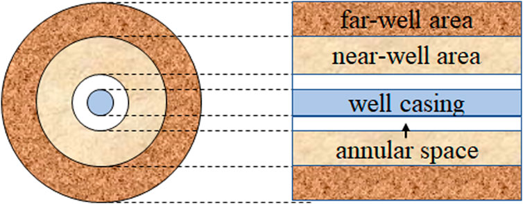
Figure 1. Reservoir-completion basic structure.

In the above, the system network composed of node analysis method and reservoir simulation grid presents the completion area and reservoir area. This model allows for the control of completion components in the modeling of complex networks. As shown in Figure 2, the location of nodes represents different identification points, and the node network of completion area or special parts is constructed to solve the problem of coupling flow between reservoir and horizontal well under different completion conditions. The boxes represent the boundaries between the nodes, and the efficiency and direction of fluid transfer is resolved by the nature of the area controlled by the nodes and the pressure difference between the areas.

Figure 2

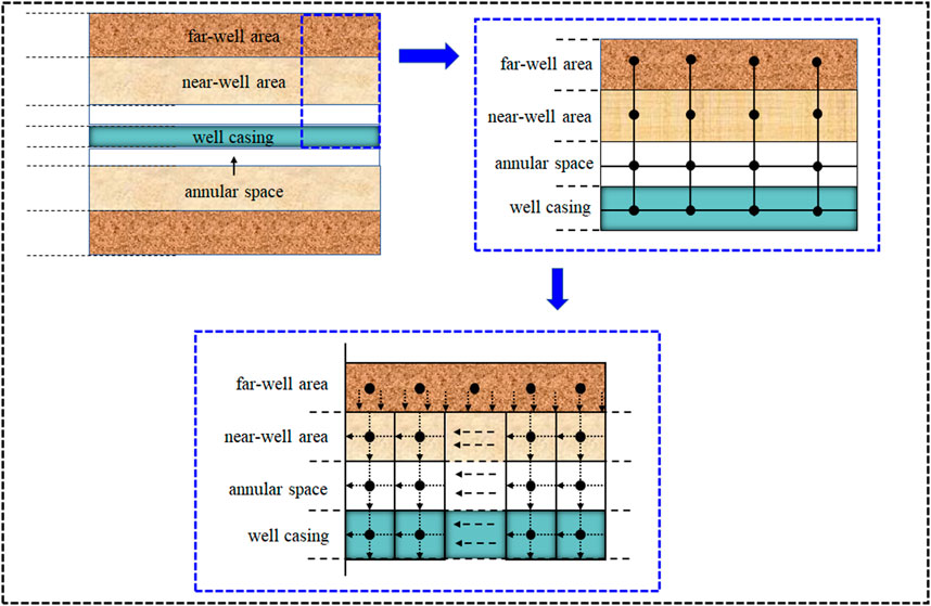
Figure 2. Well simulation grid.

3 Mathematical models for reservoir

As shown in Figure 2, only orthogonal meshing of bedrock system is needed in meshing, without considering all kinds of geometry, which avoids complex meshing and greatly reduces the amount of calculation. The problems of fluid loss and pressure loss in reservoir are solved based on Babu model (Babu and Odeh, 2013; Ma et al., 2020). The known information such as far-well reservoir pressure and horizontal well length is used as the boundary condition.

Assumptions:

(1) The flow process is constant temperature, and the fluid flow in bedrock satisfies Darcy’s law;

(2) Considering the compressibility of bedrock and fluid. The rock deformation is micro-deformation without considering the inertial force.

Compressibility calculation formula of reservoir rock:

$c_b=-\frac{1}{V^t}\frac{dV}{dP}(1)$

Productivity calculation formula:

$q=J_R\left(P_R\left(t\right)-P_r\left(t\right)\right)(2)$

$\frac{dV}{dt}=J_R\left(P_R\left(t\right)-P_r\left(t\right)\right)(3)$

The boundary formula:

$\left\{\begin{array}{c}{P}_R=P_R\left(0\right)t=0\\ P_R=P_R\left(t\right)t=t\end{array}\right.(4)$

At the same time, Equations 1–3 can be deduced:

${\int }_{P_R\left(0\right)}^{P_R\left(t\right)}\frac{dP}{\left(P_R\left(t\right)-P_r\left(t\right)\right)}=-\frac{J_R}{c_b{V}^t}{\int }_0^{t}dt(5)$

$\ln \left(\frac{P_R\left(t\right)-P_r\left(t\right)}{P_R\left(0\right)-P_r\left(t\right)}\right)=e^{\left(-\frac{J_R}{c_b{V}^t}t\right)}(6)$

$P_R\left(t\right)=P_r+\left(P_R\left(0\right)-P_r\left(t\right)\right)*e^{\left(-\frac{J_R}{c_b{V}^t}t\right)}(7)$

Formulas 8, 9 are derived from Formulas 5–7.

$P_R^{t+1}=P_r+\left(P_R^t-P_r\left(t\right)\right)*e^{\left(-\frac{J_R}{{c_{b}V}^t}∆t\right)}(8)$

$∆V=c{V}^t\left(P_R^t-P_r\left(t\right)\right)*\left(1-e^{\left(-\frac{J_R}{c_b{V}^t}∆t\right)}\right)(9)$

Figure 3 shows a schematic diagram of the physical model of horizontal wells in box formations. This article uses the Babu and Odeh models. The advantage is that for any box reservoir, the mathematical model of unstable seepage in horizontal wells is established by physical model analysis. Combined with the principle of material balance, the productivity formula of horizontal wells under quasi-steady state conditions in finite box reservoirs is given.

Figure 3

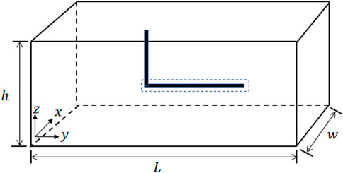
Figure 3. Schematic diagram of coupling flow between reservoir and horizontal well.

Assumptions:

(1) The reservoir with closed boundary can be regarded as a box shaped discharge area. And the length, width and height of the area are a, b, and h, respectively.

(2) Fluid flow in porous media is governed by Darcy‘s law and is slightly compressible under pressure, ignoring the effect of capillary force.

The details of the Babu and Odeh model are shown in Formulas 10–16.

$∆p\left(x,y,z,t\right)=P_r-P_t\left(x,y,z,t\right)=\frac{B\mu q}{abhL\alpha }{\int }_0^t\left[S_1\left(x_i,x_j,t\right)·S_2\left(y_i,y_j,t\right)·S_3\left(z_i,z_j,t\right)\right]d\tau (10)$

$∆p_r\left(x,y,z,t\right)=P_r-P_t\left(x,y,z,t\right)=q_{t,y}·F\left(t\right)(11)$

$F\left(t\right)=\frac{1}{\varnothing C_t}\frac{1}{abhL}{\int }_0^t\left[S_1\left(x_i,x_j,t\right)·S_2\left(y_i,y_j,t\right)·S_3\left(z_i,z_j,t\right)\right]d\tau (12)$

$S_1\left(x_i,x_j,t\right)=1+2{\displaystyle \sum _{n=1}^{\infty }}\mathit{cos}\frac{n\pi x_i}{a}\mathit{cos}\frac{n\pi x_j}{a}\exp \left(-\frac{n^2{\pi }^2{K}_{x}t}{\varnothing \mu C_t{a}^2}\right)(13)$

$S_2\left(y_i,y_j,t\right)=1+2{\displaystyle \sum _{n=1}^{\infty }}\mathit{cos}\frac{n\pi y_i}{b}\mathit{cos}\frac{n\pi y_j}{b}\exp \left(-\frac{m^2{\pi }^2{K}_{y}t}{\varnothing \mu C_t{b}^2}\right)(14)$

$S_3\left(z_i,z_j,t\right)=1+2{\displaystyle \sum _{l=1}^{\infty }}\mathit{cos}\frac{l\pi z_i}{h}\mathit{cos}\frac{l\pi z_j}{h}\exp \left(-\frac{l^2{\pi }^2{K}_{z}t}{\varnothing \mu C_t{h}^2}\right)(15)$

Set the horizontal well along the y-axis, F (t) on the y-axis is:

$F_{ij}\left(t\right)=\frac{1}{\varnothing C_t}\frac{1}{abhL}{\int }_0^t\left[S_1\left(x_0,x_0,t\right)·S_2\left(y_i,y_j,t\right)·S_3\left(z_0,z_0,t\right)\right]d\tau (16)$

Figure 4 shows the corresponding relationship between time and capacity. In the process of oil production, the flow $q_i$ at the node is constantly changing with time, and it is difficult to obtain its analytical expression. Formula 17 is used in this paper as a replacement.

$∆p_r\left(t\right)=q_{t,y}\left(t\right)*F_{ij}\left[\left(t_{i+1}-t_i\right)-\left(t_i-t_{i-1}\right)\right](17)$

Figure 4

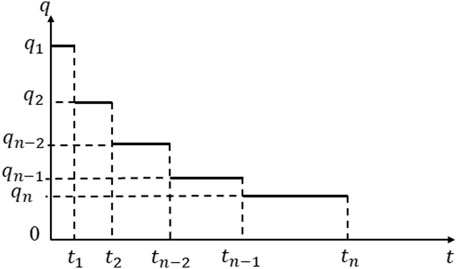
Figure 4. Discrete in time domain.

The flow at the node is regarded as uniform in the time $t=∆t$. If the time is long, the flow cannot be regarded as uniform within $t=∆t$, so the time needs to be divided into m nodes. Let $t=m∆t$, and the flow is uniform in each $∆t$. The principle of superposition can be adopted for the pressure drop of each node, and as shown in Formula 18.

$∆p_r\left(m∆t\right)={\displaystyle \sum _{j=1}^N}\begin{array}{c}{q_{\left(t,y\right)}}_j\left(∆t\right)F_{ij}\left(m∆t\right)+\left[{q_{\left(t,y\right)}}_j\left(2∆t\right)-{q_{\left(t,y\right)}}_j\left(∆t\right)\right]F_{ij}\left[\left(m-1\right)∆t\right]+\\ \dots \left\{{q_{\left(t,y\right)}}_j\left(m∆t\right)-{q_{\left(t,y\right)}}_j\left[\left(m-1\right)∆t\right]\right\}{F}_{ij}\left(∆t\right)\end{array}(18)$

The time is considered to be short enough, and the flow rate is considered to be uniform within $t=∆t$. It can be used to infer Formula 19.

$∆p_{r_i}\left(∆t\right)={\displaystyle \sum _{j=1}^n}{q_{t,y}}_j\left(∆t\right)F_{ij}\left(∆t\right)(19)$

Given that the time step is set to $∆t$, Equation 20 is discretized as follows:

$∆p_{r_i}\left({∆t}^K\right)={\displaystyle \sum _{k=1}^K}{\displaystyle \sum _{j=1}^N}{q_{t,y}}_j\left({∆t}^k\right)\left[F_{ij}\left({∆t}^K-{∆t}^{k-1}\right)-F_{ij}\left({∆t}^K-{∆t}^k\right)\right](20)$

4 Mathematical model for wellbore

4.1 Mathematical model for wellbore

Take a micro element in one-dimensional single-phase flow pipe flow as shown in Figure 5. Let the cross-sectional area of the micro-element perpendicular to the Z-axis be $A$, and its volume element be $Adz$. According to the principle of mass conservation, the difference between the mass flowing into the volume element and the mass flowing out of the volume element per unit time should be the mass change in the volume element. The fundamental formula is Equation 21, from which the other Formulas 22, 23, are inferred.

$\left(\rho +\frac{\partial \rho }{\partial z}dz\right)\left(v+\frac{\partial v}{\partial z}dz\right)Adt(21)$

Figure 5

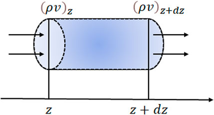
Figure 5. Unit of wellbore.

In order to speed up the solution, the second-order term can be ignored in the above equation, and the following can be obtained:

$\left(\rho +\frac{\partial \rho }{\partial z}dz\right)\left(v+\frac{\partial v}{\partial z}dz\right)Adt-\rho vAdt(22)$

Since there is no source of fluid mass in the micro-element, according to the principle of mass conservation, the variation of the volume element per unit time is equal to the net mass inflow into the micro-element, that is:

$\frac{\partial \left(\rho v\right)}{\partial z}Adzdt=-\frac{\partial \rho }{\partial t}Adzdt(23)$

4.2 Mathematical model for wellbore

As shown in Figure 6, a micro-element is taken in the flow channel pressure field. According to Newton’s second law, the change in momentum of a micro element per unit time should be equal to the sum of the external force it receives. The external forces on the micro-element include the pressure difference between the inlet and outlet ends, the frictional resistance of the pipe wall and the gravity. The relevant content is shown in Formulas 24–27.

Figure 6

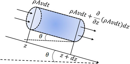
Figure 6. Momentum equation micro-element.

Pressure difference between inlet and outlet of micro-element:

$-A\frac{\partial p}{\partial z}dz(24)$

The fluid gravity in micro-element is:

$-\rho gsin\theta Adz(25)$

Friction force of fluid inside micro-element:

$-\frac{f\rho v^2}{2D}Adz(26)$

Considering the influence of gravity, friction and other factors, according to the momentum conservation principle, the following can be obtained:

$\frac{\partial \left(\rho v\right)}{\partial t}+\frac{\partial \left(p+\rho v^2\right)}{\partial z}=-\frac{f\rho v^2}{2D}-\rho gsin\theta (27)$

The friction coefficient calculation method of radial inflow is generally based on the recent research of Ouyang (1998). The calculation process is shown in Formulas 28–31.

If $R_e\le 2300$, the wall friction in laminar flow is calculated by:

For inflow case:

$f=\frac{16}{R_e}\left(1+0.04304R_{ew}^{0.6142}\right)(28)$

For outflow case:

$f=\frac{16}{R_e}\left[1-0.0625\frac{{\left(-R_{ew}\right)}^{1.3056}}{{\left(R_{ew}+4.626\right)}^{-0.2724}}\right](29)$

If $R_e\ge 2300$, the wall friction in turbulent flow is calculated by:

For inflow case:

$f=\frac{16}{R_e}\left(1-0.0153R_{ew}^{0.3978}\right)(30)$

For outflow case:

$f=\frac{16}{R_e}\left[1-17.5\frac{R_{ew}}{R_e^{0.75}}\right](31)$

5 Mathematical models for the coupling progress

The composition of this coupling model can be divided into horizontal well, completion, near-well reservoir and far-well reservoir. Therefore, the pressure loss includes the completion, casing annulus, tubing and reservoir seepage pressure loss. The fluid flow between different layers can be coupled by fluid continuity equation and momentum equation. As shown in Figure 7, the coupling model is transient in all parts of the system. Based on the specific construction of horizontal wells, the corresponding structural drawings are drawn with nodes and grids. The use of the grid can freely meet the requirements of accuracy, and gradually refine or coarsen until it meets the needs of the solution. Nodes and grids simultaneously control the orientation, region and boundary of the cell network, so that we can sort the cell structure.

Figure 7

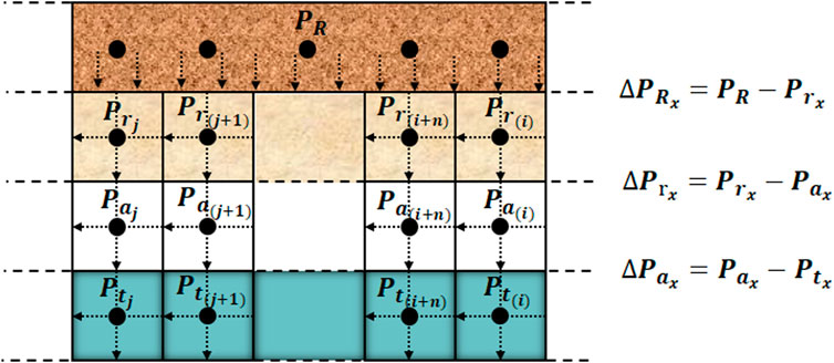
Figure 7. Discrete grid graph.

In order to simulate the change of well flow with time, the reservoir model must be combined with the well flow model. Due to the differences in reservoir properties and fluid properties at different node positions, the horizontal completion section will take corresponding completion measures. Therefore, it is necessary to establish a coupling model for different completions. The specific steps of establishing the coupling model of reservoir and different completion horizontal wells are as follows:

(1) The completion model is discretized, and the main boundary conditions are the flow pressure located at the bottom of the well and the formation pressure located in the remote reservoir. In detail, according to the length of the whole section and the completion of different positions, the horizontal section is divided into several micro-segments, and the number of nodes and network modules are set. In addition, the node position and network module control range can be arbitrarily selected according to the completion engineering requirements. At the same time, different nodes can also be refined or non-refined according to the research when dividing nodes.

(2) The flow direction of fluid in wellbore and reservoir is usually unknown. Figure 7 shows the node units in different layers, which are sorted naturally by flow direction. The ranking rules of the remaining layers are the same, but the subscripts are different. The subscript r represents the reservoir node, the subscript c represents the completion node, the subscript t represents the tubing node, and the subscripts, $j$, and $k$ represent the serial numbers respectively.

(3) Next, we can select the corresponding node unit according to the completion type and draw the coupling structure diagram. Then the nodes are sorted, and the natural sorting of the downstream direction is convenient to solve. The toe point of the horizontal well is recorded as node 1, and the nodes are sorted until the heel of the horizontal well. Other sorting methods can also be, as long as the solution variables and sort number consistent.

(4) Period setting problem of time flow. Aiming at the problem that the accuracy of the approximate model and the sampling frequency of the system cannot be taken into account when the sampling period is set synchronously to the iteration step of the approximate model, a new multi-step iteration strategy is further studied. The iteration step and sampling period of well flow and reservoir flow are set respectively, which allows multiple iteration processes in one sampling period of the approximate discrete-time model, and meets the computational accuracy requirements of the approximate discrete-time model.

(5) Solving the unknowns in the coupled model. Connecting computational equations with coupled structure diagrams, since most equations are nonlinear, an iterative method must be used.

6 Sensitivity analysis of the productivity formula and case study verification of the model

6.1 Sensitivity analysis of the productivity formula

To verify the robustness of the model, a combination of single-variable analysis and the reservoir-wellbore coupling model was employed to explore the sensitivity of influencing factors. The selected data represent steady-state conditions at a simulation time of 1 day. The model assumes a 600 m open-hole completion, with parameters listed in Table 1. As shown in Figure 8, to better evaluate the accuracy of the developed model, it was compared and analyzed against the traditional productivity model, and its productivity was observed. The Babu model is commonly used to describe the flow behavior in oil and gas wells, particularly for productivity analysis of horizontal or complex wellbores. Scholars have established a reservoir-wellbore coupled steady-state model based on the Babu model and conducted sensitivity analyses (Li et al., 2018).

Table 1

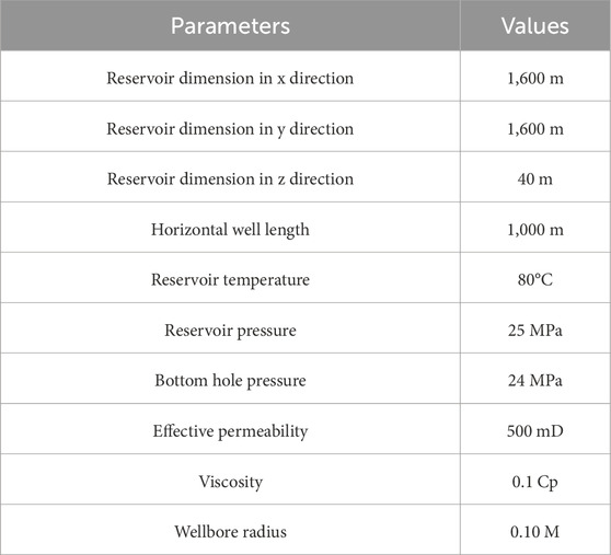
Table 1. Case study 1 parameters.

Figure 8

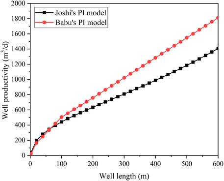
Figure 8. Comparison of pressure along the well for various productivity models.

6.2 Case study verification of the model

In this section, the results obtained after the specific application of the model are described. This example shows simulation results for a 1,000 m horizontal well. As shown in Figure 9, slotted pipes with an inner diameter of 10 cm are used for 0–300 m and 700–1,000 m, and blank pipes with an inner diameter of 10 cm are used for the middle of 300–700 m. Five groups of different time points (1 s-10 days) were selected, and the reservoir pressure in the far-well area was constant 25 MPa, and the bottomhole flow pressure was set as 24 MPa. Other parameters were shown in Table 1. In Figure 9 to Figure 14, the pressure, velocity and flow direction of the wellbore and near-well reservoirs are calculated by the solver in this paper.

Figure 9

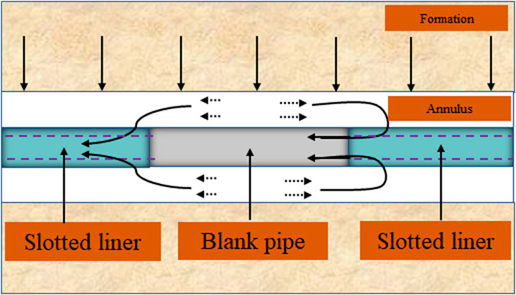
Figure 9. Well completion.

As shown in Figure 10, the dynamic evolution process of fluid entering the annulus from the reservoir is illustrated, detailing the flow profiles at different time points (1 s, 100 s, 1,000 s, and 1 day). The results indicate that the fluid flow profiles exhibit significant dynamic characteristics at different time intervals and gradually stabilize over time. Initially, at t = 1s, the rate of fluid inflow into the annulus from the reservoir is relatively uniform across segments, with an overall low flow rate, indicating that significant flow differences have not yet formed. At this stage, the inflow profile is relatively smooth, with no distinct local flow velocity peaks. Over time, the flow velocity gradually changes. At t = 100 s and t = 1,000 s, the flow velocity curves gradually approach a steady-state distribution, and the overall flow velocity exhibits nonlinear variation. Specifically, the flow velocity near the heel significantly increases, while that near the toe is relatively lower. This asymmetric inflow profile is caused by pressure drops and local resistance variations within the annulus. Figure 11 illustrates the axial flow of fluid within the annulus. At the initial moment (t = 1 s), the flow velocity near the heel (0 m) is low. As the distance increases to 100 m, the velocity rises rapidly, reaching a peak in the 150 m–300 m range before gradually decreasing. At t = 100 s, the overall flow velocity increases significantly, and velocity differences between positions become more pronounced. At t = 1,000 s, except for the gradual decline in flow velocity near the heel, the flow velocity in the middle and rear sections stabilizes, and the system approaches steady-state conditions.

Figure 10

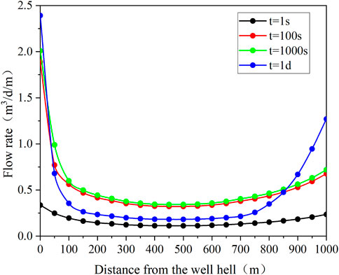
Figure 10. Flow rate reservoir to annulus.

Figure 11

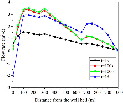
Figure 11. Axial flow rate in annulus.

Figure 12 describes the axial flow of fluid in the tubing. In this coupling model, the positive direction of well inflow refers to the flow direction from the near-well reservoir to the annulus and the annulus to the wellbore, and the axial flow of each interval is defined as the positive direction from the toe to the heel. As shown in Figure 10, when t = 1 day, the axial flow of the annulus near the heel is negative, which means that in the part of about 100 m from the heel, the fluid flows from the heel to the toe. Figure 13 shows the evolution of tubing pressure. It is observed from Figure 13 that there is a sharp change of pressure, corresponding to two flow jumps in Figure 11. At the same time, it can be observed that the flow field and pressure field in the tubing tend to be stable at t = 1000s.

Figure 12

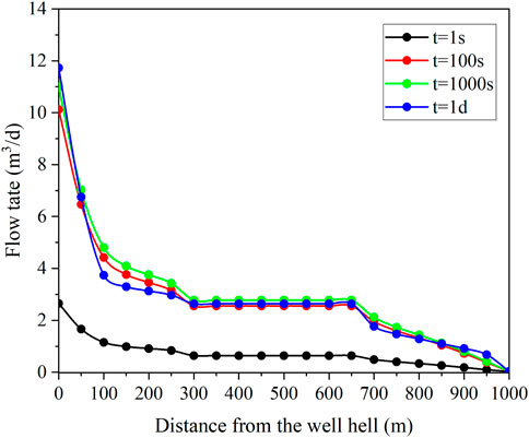
Figure 12. Axial tubing flow rate.

Figure 13

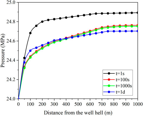
Figure 13. Tubing pressure distribution.

Figure 14 and Figure 15 show the reservoir pressure at the corresponding position in the reservoir and the axial flow in the reservoir, respectively. As can be seen from the picture, it takes longer for the transient state to reach steady state. In fact, in the model constructed this time, the near-well reservoir still does not reach a stable state at t = 10 h, and the time required to reach a stable state in the reservoir is much longer than in the well.

Figure 14

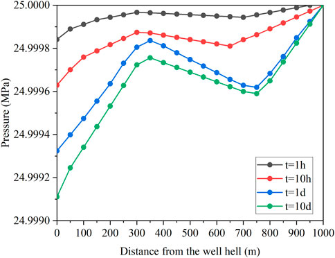
Figure 14. Reservoir pressure distribution.

Figure 15

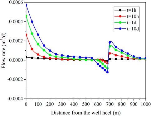
Figure 15. Axial flow rate in reservoir.

7 Conclusion

This paper effectively controls the interactions between different layers using a nodal discretization method, thereby addressing the unsteady flow coupling problem between horizontal wells and the reservoir. To achieve this, the flow states of the horizontal wellbore and the reservoir are solved separately in transient and steady-state phases, enabling the capture of dynamic responses inside the wellbore and the description of seepage characteristics in the near-well region. The conclusions are as follows:

(1) Based on fluid mechanics and reservoir seepage theories, this paper establishes an unsteady flow coupling model that includes the horizontal wellbore, completion structure, and near-well reservoir. By considering the dynamic seepage characteristics of the near-well reservoir, the model systematically analyzes the pressure distribution and flow rate variations inside the wellbore and near the well region. This model allows for a more accurate description of the complex dynamic response processes of horizontal wells and their surrounding reservoirs.

(2) The pressure and flow velocity in the wellbore, annulus, and near-well reservoir were calculated and analyzed. The results show that the entire coupled system takes more than 10 h to stabilize, while the local stabilization time of the wellbore and annulus is about 1,000 s. Notably, during this process, the axial flow velocity near the heel of the annulus exhibits negative values, indicating reverse fluid flow from the heel to the toe. This phenomenon is highly consistent with the complex flow behavior observed in actual oil fields, confirming the effectiveness and practicality of the model in describing horizontal wellbore flow characteristics.

(3) By comparing the flow and pressure field distributions at different times, this paper provides a detailed characterization of the dynamic response features of various sections at given moments. The results indicate that the new model has high practical value in predicting the dynamic response of horizontal wells under different completion parameters, offering a theoretical basis for optimizing completion parameters and improving recovery in actual oil field development.

This study offers a new approach to dynamic coupling modeling of horizontal wells and reservoirs, particularly in describing the flow characteristics of the wellbore and reservoir during the early transient stage, providing guidance for dynamic oilfield management and enhanced recovery. However, the model still has shortcomings in transient descriptions during the early stages, mainly in its inability to accurately reflect the dynamic responses of both the wellbore and the near-well reservoir simultaneously. This limitation may affect the prediction accuracy of early-stage results.

Data availability statement

The original contributions presented in the study are included in the article/supplementary material, further inquiries can be directed to the corresponding author.

Author contributions

ZC: Conceptualization, Methodology, Writing – original draft, Writing – review & editing. JL: Software, Validation, Writing – review & editing. LZ: Formal Analysis, Validation, Writing – review & editing. KZ: Data curation, Resources, Writing – review & editing. CL: Writing – original draft, Writing – review & editing. ZH: Project administration, Visualization, Writing – review & editing. XD: Supervision, Writing – review & editing.

Funding

The author(s) declare that no financial support was received for the research and/or publication of this article.

Conflict of interest

Authors ZC, JL, LZ, KZ, CL, ZH, and ZD were embloyed by CNOOC Ener Tech-Drilling & Production Co.

Generative AI statement

The author(s) declare that no Generative AI was used in the creation of this manuscript.

Publisher’s note

All claims expressed in this article are solely those of the authors and do not necessarily represent those of their affiliated organizations, or those of the publisher, the editors and the reviewers. Any product that may be evaluated in this article, or claim that may be made by its manufacturer, is not guaranteed or endorsed by the publisher.

References

Ahammad, M. J., Rahman, M. A., Alam, J., and Butt, S. (2019). A computational fluid dynamics investigation of the flow behavior near a wellbore using three-dimensional Navier–Stokes equations. Adv. Mech. Eng. 11 (9). doi:10.1177/1687814019873250

CrossRef Full Text | Google Scholar

Babu, D. K., and Odeh, A. S. (2013). Productivity of a horizontal well. SPE Reserv. Eng. 4 (4), 417–421. doi:10.2118/18298-pa

CrossRef Full Text | Google Scholar

Cao, J., Zhang, N., and Johansen, T. E (2019). Applications of fully coupled well/near-well modeling to reservoir heterogeneity and formation damage effects. J. Petroleum Sci. Eng. 176, 640–652. doi:10.1016/j.petrol.2019.01.091

CrossRef Full Text | Google Scholar

Clarkson, C. R., Qanbari, F., and Williams-Kovacs, J. D. (2016). Semi-analytical model for matching flowback and early-time production of multi-fractured horizontal tight oil wells. SPE/AAPG/SEG Unconventional Resources Technology Conference. OnePetro. doi:10.1016/j.juogr.2016.07.002

CrossRef Full Text | Google Scholar

Dikken, B. J (1990). Pressure drop in horizontal wells and its effect on production performance. J. petroleum Technol. 42 (11), 1426–1433. doi:10.2118/19824-PA

CrossRef Full Text | Google Scholar

Fokker, P. A., and Verga, F. (2013). A semianalytic model for the productivity testing of multiple wells. SPE Reserv. Eval. &Engineering 11 (3), 466–477. doi:10.2118/94153-pa

CrossRef Full Text | Google Scholar

Fu, Y. (2019). A critical productivity equation of horizontal wells in a bottom water drive reservoir with low-permeability interbeds. Arabian J. Geosciences 12 (24), 758–765. doi:10.1007/s12517-019-4930-y

CrossRef Full Text | Google Scholar

Guo, B., Yu, X., and Khoshgahdam, M (2009). Simple analytical model for predicting productivity of multifractured horizontal wells. SPE Reserv. Eval. & Eng. 12 (06), 879–885. doi:10.2118/114452-pa

CrossRef Full Text | Google Scholar

Holmes, J. A., Barkve, T., and Lund, O. (1998). Application of a multisegment well model to simulate flow in advanced wells[C]. European petroleum conference. OnePetro. doi:10.2118/50646-MS

CrossRef Full Text | Google Scholar

Johansen, T. E., James, L., and Cao, J (2015). Analytical coupled axial and radial productivity model for steady-state flow in horizontal wells. Int. J. Petroleum Eng. 1 (4), 290. doi:10.1504/ijpe.2015.073538

CrossRef Full Text | Google Scholar

Johansen, T. E., and Khoriakov, V (2007). Iterative techniques in modeling of multi-phase flow in advanced wells and the near well region. J. Petroleum Sci. Eng. 58 (1-2), 49–67. doi:10.1016/j.petrol.2006.11.013

CrossRef Full Text | Google Scholar

Joshi, S. D. (1988). Augmentation of well productivity with slant and horizontal wells. J. Petroleum Technol. 8 (6), 729–739. doi:10.2118/15375-PA

CrossRef Full Text | Google Scholar

Ju, Y., Wang, Y., Chen, J., and Gao, F (2018). Adaptive finite element-discrete element method for numerical analysis of the multistage hydrofracturing of horizontal wells in tight reservoirs considering pre-existing fractures, hydromechanical coupling, and leak-off effects. J. Nat. Gas Sci. Eng. 54, 266–282. doi:10.1016/j.jngse.2018.04.015

CrossRef Full Text | Google Scholar

Khoriakov, V., Johansen, A. C., and Johansen, T. E (2012). Transient flow modeling of advanced wells. J. Petroleum Sci. Eng. 86, 99–110. doi:10.1016/j.petrol.2012.03.001

CrossRef Full Text | Google Scholar

Kong, X., and McAndrew, J. (2017). A computational fluid dynamics study of proppant placement in hydraulic fracture networks. SPEU nconventional resources conference. OnePetro. doi:10.2118/185083-MS

CrossRef Full Text | Google Scholar

Krogstad, S., and Durlofsky, L. J (2009). Multiscale mixed-finite-element modeling of coupled wellbore/near-well flow. SPE J. 14 (01), 78–87. doi:10.2118/106179-PA

CrossRef Full Text | Google Scholar

Kurtoglu, B., Medeiros, F., Ozkan, E., and Kazemi, H. (2008). “Semianalytical representation of wells and near well flow convergence in numerical reservoir simulation,” in SPE annual technical conference and exhibition, China, September 21 2008. doi:10.2118/116136-MS

CrossRef Full Text | Google Scholar

Li, H., Tan, Y., Jiang, B., Wang, Y., and Zhang, N (2018). A semi-analytical model for predicting inflow profile of horizontal wells in bottom-water gas reservoir. J. Petroleum Sci. Eng. 160, 351–362. doi:10.1016/j.petrol.2017.10.067

CrossRef Full Text | Google Scholar

Ma, G., Wu, X., Han, G., Xiong, H., and Xiang, H (2020). A semianalytical coupling model between reservoir and horizontal well with different well completions. Geofluids 2020 (1), 1–12. doi:10.1155/2020/8890174

CrossRef Full Text | Google Scholar

Ming, C., Zhang, S., Yun, X. U., Ma, X., and Zou, Y (2020). A numerical method for simulating planar 3D multi-fracture propagation in multi-stage fracturing of horizontal wells. Petroleum Explor. Dev. 47 (1), 171–183. doi:10.1016/S1876-3804(20)60016-7

CrossRef Full Text | Google Scholar

Munkejord, S. T., Hammer, M., Ervik, Å., Odsæter, L. H., and Lund, H (2021). Coupled CO 2-well-reservoir simulation using a partitioned approach: effect of reservoir properties on well dynamics. Greenh. Gases Sci. Technol. 11 (1), 103–127. doi:10.1002/ghg.2035

CrossRef Full Text | Google Scholar

Nie, R. S., Ou, J. J., Wang, S. R., Deng, Q., Qin, M., Jia, J. W., et al. (2018). Time-tracking tests and interpretation for a horizontal well at different wellbore positions. Interpretation 6 (3), T699–T712. doi:10.1190/INT-2017-0213.1

CrossRef Full Text | Google Scholar

Ouyang, L. B. (1998). Single-phase and multiphase fluid flow in horizontal wells. Stanford University.

Google Scholar

Peng, L., Han, G., Chen, Z., Pagou, A., Zhu, L., and Abdoulaye, A (2022). Dynamically coupled reservoir and wellbore simulation research in two-phase flow systems: a critical review. Processes 10 (9), 1778. doi:10.3390/pr10091778

CrossRef Full Text | Google Scholar

Ranjith, R., Suhag, A., Balaji, K., Putra, D., Dhannoon, D., Saracoglu, O., et al. (2017). Production optimization through utilization of smart wells in intelligent fields. SPE Western regional meeting. doi:10.2118/185709-MS

CrossRef Full Text | Google Scholar

Rooki, R., Doulati Ardejani, F., Moradzadeh, A., and Norouzi, M (2014). Simulation of cuttings transport with foam in deviated wellbores using computational fluid dynamics. J. Petroleum Explor. Prod. Technol. 4 (3), 263–273. doi:10.1007/s13202-013-0077-7

CrossRef Full Text | Google Scholar

Sheng, G., Javadpour, F., Su, Y., Liu, J., Li, K., and Wang, W. (2019). Asemi-analytic solution for temporal pressure and production rate in a shale reservoir with nonuniform distribution of induced fractures. SPE J. 24 (4), 1856–1883. doi:10.2118/195576-PA

CrossRef Full Text | Google Scholar

Szanyi, M. L., Hemmingsen, C. S., Yan, W., Walther, J. H., and Glimberg, S. L (2018). Near-wellbore modeling of a horizontal well with computational fluid dynamics. J. Petroleum Sci. Eng. 160, 119–128. doi:10.1016/j.petrol.2017.10.011

CrossRef Full Text | Google Scholar

Tiab, D., and Donaldson, E. C. (2024). Petrophysics: theory and practice of measuring reservoir rock and fluid transport properties. Elsevier.

Google Scholar

Vicente, R., Sarica, C., and Ertekin, T. (2000). A numerical model coupling reservoir and horizontal well-flow dynamics: transient behavior of single-phase liquid and gas flow. Pa. State Univ. 7, 70–77. doi:10.2118/77096-PA

CrossRef Full Text | Google Scholar

Wang, N., Sun, B., Wang, Z., Wang, J., and Yang, C. (2016). Numerical simulation of two phase flow in wellbores by means of drift flux model and pressure based method. J. Nat. Gas Sci. Eng. 36, 811–823. doi:10.1016/j.jngse.2016.10.040

CrossRef Full Text | Google Scholar

Yao, S., Zeng, F., Liu, H., and Zhao, G. (2012). “A semi-analytical model for multi-stage fractured horizontal wells,” in SPE Canadian unconventional resources conference, Canada, March 18, 2020 (OnePetro). doi:10.1016/j.jhydrol.2013.10.033

CrossRef Full Text | Google Scholar