The effect of PV modules on temperature conditions of nearby power cables

The highest permissible load of power cables (ampacity) depends strongly on the ambient temperature, which in the case of cables surrounded by free air is generally assumed to be 25°C. Considering the installation of photovoltaic (PV) modules, the thermal conditions for the cables connected to these modules may be very unfavorable. The cables are laid under the module and the space underneath it is heated by this module. The aim of the paper is to present a numerical model of an example PV module mounted on the roof of a building, as well as the results of numerical calculations of the temperature around the module. Based on the numerical model of the PV system and advanced calculations it is possible to introduce a correction factor to determine the ampacity of the power cables located in the vicinity of the PV module. The authors’ research allows for the correct determination of the cable ampacity, avoiding its overheating and preventing the risk of fire.

1 Introduction

The highest permissible load of power cables (ampacity) depends on many factors, including the material and cross-section of the cable core, ambient temperature, the continuously permissible temperature related to the insulation material, the mutual distance between cables arranged in bundles and the method of laying cables (in the ground, surrounded by free air or in cable ducts) (de Leon, 2006; Holyk and Anders, 2015; Papadopoulos et al., 2023). For cables laid in the ground, the thermal parameters of the soil are of crucial importance (Jiang et al., 2023; Drefke et al., 2021). It is also important at what depth the cables are laid (Baazzim et al., 2014; Klimenta et al., 2018), whether there are more cable bundles that interact with each other (Xiong et al., 2019) as well as what method of cable sheaths bonding is used, which, due to the induced voltages/currents, may influence on the temperature of the cable insulation (Akbal, 2018) or may cause damage of the cable terminations (Akbal, 2019). In the case of overhead conductors (Zenczak, 2017; Girshin et al., 2020) and insulated cables surrounded by free air (Bin Wan Mohd Zain et al., 2022), it is very important to properly determine the air temperature in the vicinity of the cables/conductors and take into account possible direct sunlight (Czapp et al., 2017). The influence of solar radiation on the ampacity of cables also applies to underground cable lines–in modeling of low-voltage cables (Klimenta et al., 2018) it was shown that this ampacity depends on the type of ground surface (asphalt, concrete block, color of pavement surface). Moreover, comparative analyses of calculations related to the design of cable lines in the context of their ampacity vs. field experimental studies based on the Distributed Temperature Sensing system have shown that the assumptions adopted in the calculations may significantly differ from the actual conditions (Strand et al., 2023). Comparison of cables laid in the ground vs. surrounded by free air (Hu et al., 2024) shows significant discrepancies in their ampacity, because the conditions of heat dissipation from the cables are different. Very unfavorable temperature conditions for cables are in the case of their installation on a sunny roof, as shown in Brender and Lindsey (2008). In the case of laying cables in pipes on the roof, just sunlight can increase the temperature of their interior by approximately 40°C. As it results from the analysis carried out in Czapp et al. (2018), the sun and still air around the electrical installation can provide more unfavorable conditions for heat dissipation from cables than the standards considered. This can lead to thermal damage of the cable insulation. Very similar conditions occur in the case of photovoltaic (PV) installations and associated cables, which are the subject of this paper. PV modules are sources of significant heat emitted from both the upper and lower surfaces. The test results presented in Perovic et al. (2019) indicate that the PV module temperature can be close to 75°C. In the case of PV systems, damage to cable insulation is particularly dangerous. This can cause a fire (Falvo and Capparella, 2015), and extinguishing it is a challenge for the firefighters–the PV system contains autonomous energy sources generating output voltage despite damage, and extinguishing them poses a risk of electrocution (Backstrom and Dini, 2011; Tommasini et al., 2014). It is therefore important to apply calculation methods based on advanced numerical modeling in order to correctly determine the thermal conditions around the cables, which affect their ampacity (Enescu et al., 2020; Cywinski and Chwastek, 2021). This issue is important due to the commonness of PV installations and, consequently, the potential fire hazard for many buildings (mainly residential) where such installations are located. The aim of this paper is to fill the gap related to a more accurate representation of the possible air temperature surrounding the cables near the PV modules. This will allow to indicate the realistic values of the ampacity correction factor depending on the predicted temperature of this air. Numerical studies and the computation of the ampacity values were performed for an example PV installation placed on the roof of a building. The contribution of this manuscript is the results of numerical modeling and calculated values for correcting the ampacity of cables associated with the PV system.

The rest of the paper is organized as follows. Section 2 shows the model of the tested PV system, the assumptions for numerical modeling as well as the results of numerical calculations related to the temperature around the PV module. Section 3 defines the cable ampacity correction factor and presents the proposed values of this factor based on numerical calculations. Section 4 presents the research conclusions.

2 Ambient temperature, investigated model and results of numerical calculations

2.1 Ambient temperature

In the case of power cables surrounded by free air, not exposed to direct solar radiation, the ampacity is expressed by the following relationship (IEC 60287, 1999, 2023):

$I_{\text{amp}}=\sqrt{\frac{\Delta \theta -W_{\mathrm{d}}\cdot \left[0.5\cdot T_1+n_{\mathrm{c}}\cdot \left(T_2+T_3+T_4\right)\right]}{R\cdot T_1+n_{\mathrm{c}}\cdot R\cdot \left(1+{\lambda }_1\right)\cdot T_2+n_{\mathrm{c}}\cdot R\cdot \left(1+{\lambda }_1+{\lambda }_2\right)\cdot \left(T_3+T_4\right)}}(1)$

where I_amp–ampacity, A,

n_c–number of conductors in a cable,

R–AC current resistance of a conductor at its maximum operating temperature, Ω/m,

T₁–thermal resistance per core between the conductor and sheath, (K⋅m)/W,

T₂–thermal resistance between the sheath and armour, (K⋅m)/W,

T₃–thermal resistance of external serving of the cable, (K⋅m)/W,

T₄–external thermal resistance between the cable surface and the surrounding medium, (K⋅m)/W,

W_d–dielectric losses per unit length per phase, W/m,

ΔΘ–permissible temperature rise of the conductor above ambient temperature, K,

λ₁–ratio of the total losses in metallic sheaths to the total conductor losses,

λ₂–ratio of the total losses in metallic armour to the total conductor losses.

If we consider low-voltage power cables, including those used in photovoltaic installations, expression (Equation 1) can be simplified to:

$I_{\text{amp}}=\sqrt{\frac{\Delta \theta }{R\cdot \left(T_3+T_4\right)}}(2)$

In the expressions (Equations 1 and 2) there is a permissible temperature increase Δθ of the cable above the ambient temperature. This parameter can be written in a different way, so that in the expression (Equation 3) there is the ambient temperature τ_o and the continuously permissible temperature of the cable τ_max:

$I_{\text{amp}}=\sqrt{\frac{{\tau }_{\max }-{\tau }_{\mathrm{o}}}{R\cdot \left(T_3+T_4\right)}}(3)$

where

I_amp, R, T₃, T₄–as in expression (Equation 1), τ_max–continuously permissible temperature of the cable, K (°C), τ_o–normalized ambient temperature, K (°C).

The insulation of low-voltage power cables is usually made of polyvinyl chloride (PVC) or cross-linked polyethylene (XLPE). If a very high level of the continuously permissible temperature is required, then silicone rubber insulated cables are used. The values of the above-mentioned permissible temperature τ_max of selected insulation materials are as follows:

• polyvinyl chloride: 70°C,

• cross-linked polyethylene: 90°C,

• silicone rubber: 180°C.

The ampacity depends to a large extent on the ambient temperature. This temperature for selected countries is given in Table 1. Example of annual temperature variation during 1 year in a relatively warm region (Pakistan) is shown in Figure 1. As you can see, the highest temperatures during the year are close to 45°C (“Maximum Temperature” curve). Even in the case of the lowest recorded temperatures (“Minimum Temperature” curve), there are periods during the year when the temperature does not drop significantly below 30°C. The monthly average high is 39.3°C and 23.4°C in case of highest (“Maximum Temperature”) and lowest (“Minimum Temperature”) recorded temperatures respectively. It is obvious that the cables close to the heat source will be subjected to consistently high ambient temperatures which is detrimental to the safe operation of PV system. If incorrectly estimated, such high ambient temperatures may lead to thermal damage to electrical installation components, including cables.

Table 1

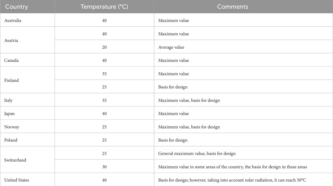
Table 1. Ambient air temperature–maximum or used as design basis for selected countries; based on (IEC 60287, 1999, 2023).

Figure 1

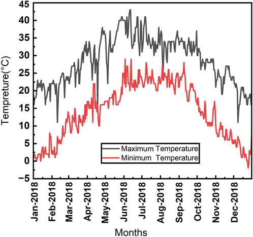
Figure 1. Annual temperature variability in Pakistan for the year 2018; own elaboration based on (Sabir et al., 2024) – data from Climate, Energy and Water Research Institute (CEWRI) field station, National Agricultural Research Centre (NARC), Islamabad, Pakistan.

In some countries, e.g., in Finland, Norway, Poland, the ambient air temperature (basis for design) is assumed to be 25°C and this value will be further taken as reference. However, in the case of PV modules, the thermal conditions for the cables connected to these modules can be very unfavorable. The cables are laid under the module, and the module exerts thermal influence on the cables. This causes an increase in the air temperature around the cable, even though the cable and its immediate surroundings are shielded from direct sunlight. These unfavorable conditions for cables connected to photovoltaic modules are reflected in the requirements of the standard (IEC 60364-7-712, 2017). This standard indicates that when selecting cables that can be heated by the heat flux emitted by the lower surface of the module, the ambient temperature for the cables may be very high and this has to be taken into account when calculating the ampacity. This shows that the effect of the high temperature of the PV module on the cables is very important. In the next subsection the investigated PV system model is described and the results of numerical calculations are discussed.

2.2 Description of the investigated model and results of numerical calculations

A simplified model of the tested PV system is shown in Figure 2. It was assumed that a photovoltaic module with a maximum power of 455 W was placed on a roof having a pitch angle of 30°, covered with cement roof tiles. The most important data of the tested system are included in Table 2. The ambient temperature was assumed to be 25°C, which is the temperature usually considered in many countries when determining the ampacity of power cables surrounded by free air (IEC 60287, 1999, 2023). The model assumed that the distance between the lower surface of the PV module and the roof surface is constant and equal to 40 mm. There is a power cable in the space between the module and the roof–this cable is in the upper part of the system (Figure 2).

Figure 2

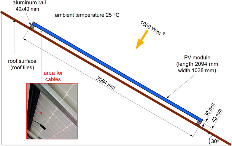
Figure 2. Diagram showing the arrangement of a PV module with a maximum power of 455 W, along with the basic parameters of the tested system (including an illustrative photo with the cable connected).

Table 2

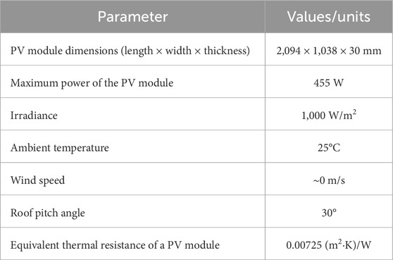
Table 2. The parameters of the analyzed system adopted for numerical calculations, based on Gaitho et al. (2009), Ruiz-Reina et al. (2014), and Znshinesolar 9BB half-cell (2024).

The investigation assumed that the cable was not loaded with current, in order to examine only the thermal effect of the PV module on the cable insulation. Thanks to this, there is no need to take into account the additional heat flux that would be generated by the current flowing in the cable. The system shown in Figure 2 was modeled in ANSYS Fluent. First, the two-dimensional geometry of the system was mapped, including the PV module, the glass layers on both sides of the module, the supporting aluminum rails, the air below the module, the air above the module, the roof of the building, and the cable below the PV module. In order to perform the calculations, a triangular computational mesh was generated, which was densified in the vicinity of the PV module. The mesh independence test was performed on three different grids with different numbers of elements, and specific results are presented in Table 3. During the mesh independence test, the maximum temperature in the whole domain was monitored and the calculations were stopped after it reached stable value. The computational time had increased nearly 60 times for the finest mesh (1,080·10³ vs. 125·10³ elements) so using a coarse mesh of 125·10³ elements can be a quite good compromise between accuracy of the results and computational effort but for the purpose of further calculations the 440·10³ element mesh was chosen.

Table 3

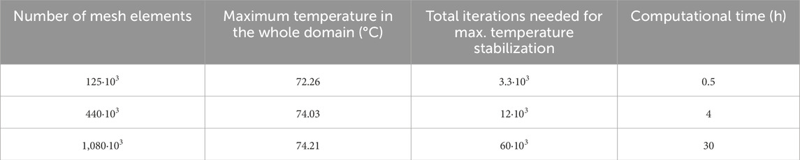
Table 3. Data related to the grid independence test.

The size of the computational mesh cells on the longer side of the PV module was set to 0.5 and 0.2 mm on the shorter side, and even smaller cells were generated on the circumference of the cable placed under the PV module. In order to correctly represent the convective heat exchange, a boundary layer was generated at the points of contact between the air and the PV module. The entire computational mesh consisted of over 440·10³ elements, and Figure 3 shows its close-up in the vicinity of the upper part (Figure 3A) and lower part (Figure 3B) of the PV module, with a visible cable (clear white dot in Figure 3A).

Figure 3

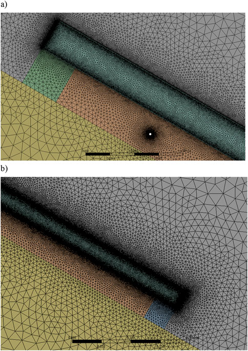
Figure 3. View of the tested model developed in ANSYS Fluent: (A) upper part of the model with power cable, (B) lower part of the model.

The finite element (FE) mesh was applied into ANSYS Fluent, where steady-state calculations of air flow and heat transfer were performed. To model natural convection correctly, the effect of gravity and the variable air density depending on temperature were taken into account, with the density being described by the ideal gas equation. The k-epsilon turbulence model was used and the energy equation was activated, which allowed to perform heat transfer simulation and obtain temperature field in whole computational domain. The discrete ordinates (DO) radiation model was activated in order to include thermal radiation of hot surfaces in the model. The thermal properties of all materials were included in the model and are presented in Table 4. The roof was defined as a homogeneous material for the entire thickness, which was the simplification of the model as the cross-section of every house can be different. In general, it can be assumed that under the thin layer of cement roof tiles there is a thicker concrete layer. The thermal conductivity of both materials is nearly the same, so the thermal conductivity of this whole body was set to 1.5 W/(m·K).

Table 4

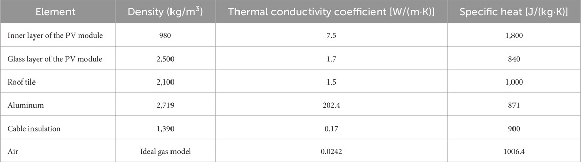
Table 4. Comparison of the selected physical properties for the analyzed materials, based on EN 12524 (2000) and Ruiz-Reina et al. (2014).

The “pressure outlet” condition was given on the external surfaces of the system (right side, left side and top) so that the air could freely flow in and out of the calculation area, which made it possible to represent convection currents in windless conditions. On the top surface of the PV module, below the glass layer, the heat flux (1,000 W/m²) provided by solar radiation was applied. The discretization schemes used were “body force weighted” for pressure and second-order for other quantities. Then, numerical calculations were performed and the max. temperature was monitored in order to achieve proper solution.

As expected, the region with the highest temperatures is the PV module itself and the space directly below it. Due to the fact that the cable is placed very close to the bottom surface of the PV module (the point representing the cable is indicated by an arrow in Figure 4B), it is necessary to significantly correct the cable ampacity in relation to the arrangement of the cables in air at a commonly assumed ambient temperature (25°C).

Figure 4

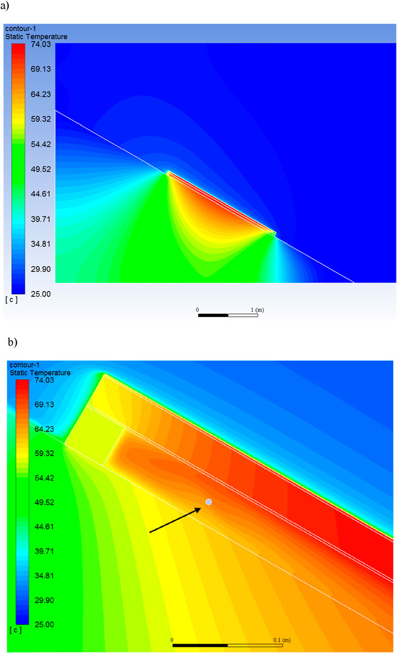
Figure 4. Temperature distribution (°C) around the PV module: (A) view of the entire system, (B) enlargement of the upper part of the space under the module containing the cable. Maximum temperature around the PV module: 74.03°C. The cable in the space under the module is not loaded with current.

When it comes to air movement near the PV module (Figure 5), due to the hot upper surface of the PV module, convection currents appear and heated air accelerates alongside the module. As the air, while heated decreases its density, the buoyancy force appears and its movement is forced from right bottom corner to left upper corner according to Figure 5B. The maximal velocity is observed above the middle section of the module and for the analyzed case it reaches the value of 0.32 m/s. The enhanced velocity region has the width of 100 mm above the PV module and length slightly shorter than the module. In the initial section alongside the PV module (right bottom corner in Figure 5) the cold air is being heated and accelerates. In the middle section of the module the increase of air temperature is not so intense due to the lower temperature difference between air and module surface and the air velocity is almost constant. The presence of convection significantly enhances the heat transfer efficiency compared to motionless air. In the numerical model, the convection process not only appears above the PV module. Between the module and the roof of the building, there is also visible some circulation of air. For the analyzed 2D case, the volume of air below the module is separated by the module supports and the inflow of fresh air is totally blocked as well as the outflow. For some real cases, the situation can be different and more favourable–the fresh air can flow through side holes alongside the module. However, in general using the PV module support situated crosswise to the module partially blocks the convective currents in air volume below the module. Therefore, the authors’ aim is to present the worst-case scenario (no ventilation of the module from the bottom), which provides the safest approach to PV system design.

Figure 5

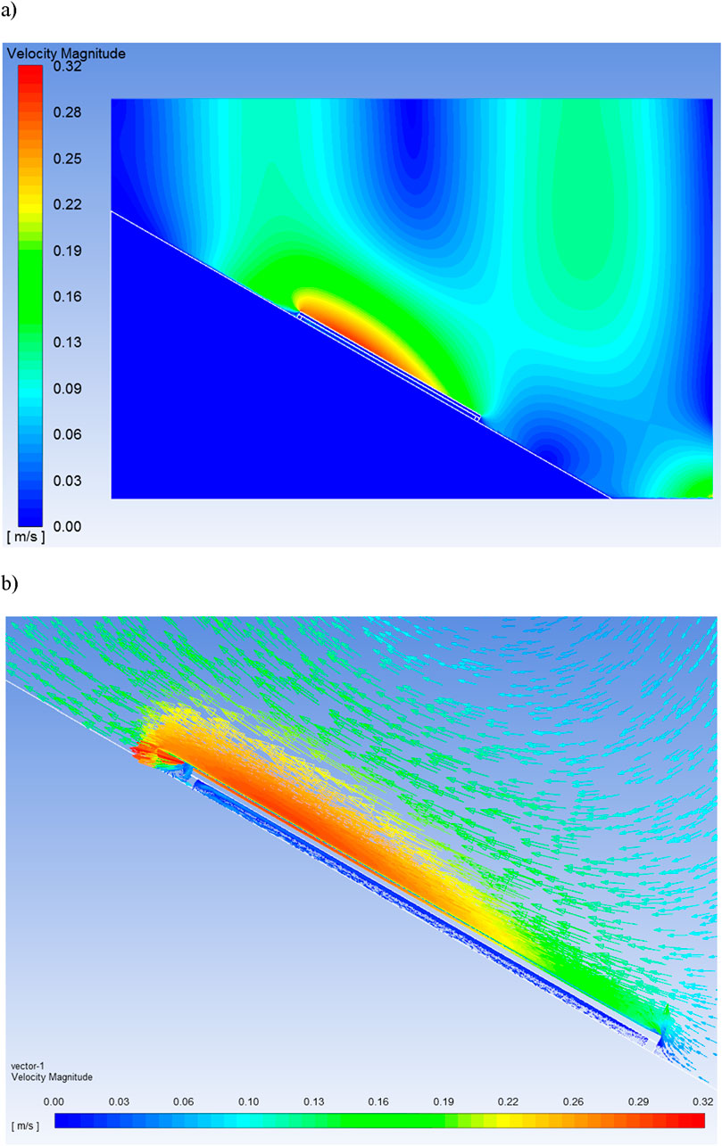
Figure 5. Velocity distribution (m/s) of the surrounding air (A) and enlargement showing the air velocity vectors (B).

3 Reduction of the ampacity of power cables

Taking into account the results of the numerical analysis presented in Section 2, in the case of cables installed near PV modules, and especially under them, it is necessary to correct the ampacity due to the high temperature around these cables. The correction (reduction) of the ampacity I_amp-PV for a given temperature τ_o-PV can be made (Musial, 2008) by multiplying the ampacity I_amp at the standardized temperature τ_o = 25°C by the following correction factor w_k:

$I_{\text{amp}–\text{PV}}=I_{\text{amp}}{·w}_{\mathrm{k}}(\mathrm{4a})$

$w_{\mathrm{k}}=\frac{1}{\sqrt{\frac{{\tau }_{\max }-{\tau }_{\mathrm{o}}}{{\tau }_{\max }-{\tau }_{\mathrm{o}-\text{PV}}}}}(\mathrm{4b})$

where

I_amp–ampacity at the standardized ambient temperature (here 25°C),

I_amp-PV–ampacity for increased temperature around cables,

w_k–correction factor (−),

τ_max–continuously permissible temperature of the cable, K (°C),

τ_o–normalized ambient temperature, K (°C),

τ_o-PV–temperature close to the cable, K (°C).

The values of the correction factor for cables with the two most popular insulation materials (PVC and XLPE) are shown in Figure 6. If the temperature around the cables is 60°C, the value of the correction factor for XLPE is about 0.7, while for PVC it is slightly below 0.5. A PVC insulated cable could therefore be loaded with current of less than 50% in relation to the nominal conditions, at which the ambient temperature is 25°C.

Figure 6

Figure 6. Values of the ampacity correction factor depending on the ambient temperature close to the cables. XLPE–cross-linked polyethylene insulated cable (the continuously permissible temperature is 90°C); PVC–polyvinyl chloride insulated cable (the continuously permissible temperature is 70°C).

Based on the calculated values of the correction factor, a table of ampacity of cables with selected cross-sections of copper conductors (as an example) was developed (Table 5). This table allows the selection of the cables cross-section when they are to be installed near PV modules and high temperature around the cables is expected. If it is necessary to run cables other than solar cables on the roof, in the immediate vicinity of photovoltaic modules, e.g., to power devices not related to the photovoltaic installation, PVC insulated cables are generally excluded. If the temperature surrounding the cable is assumed to be the maximum value obtained from numerical calculations (approximately 74°C–75°C), then these cables (PVC insulated) cannot be loaded with current at all. Cross-linked polyethylene (XLPE) insulated cables can be used, but the correction in ampacity will be significant. In the case of a 6 mm² cable, its ampacity at a surrounding air temperature of 75°C is 29.0 A compared to an ampacity of 60.4 A at a surrounding air temperature of 25°C. It seems reasonable to prepare a similar ampacity table for other cable cross-sections typically used in solar and domestic installations. This would allow designers and installers of such installations to select the correct cables to avoid overheating and, consequently, the risk of electric shock or fire.

Table 5

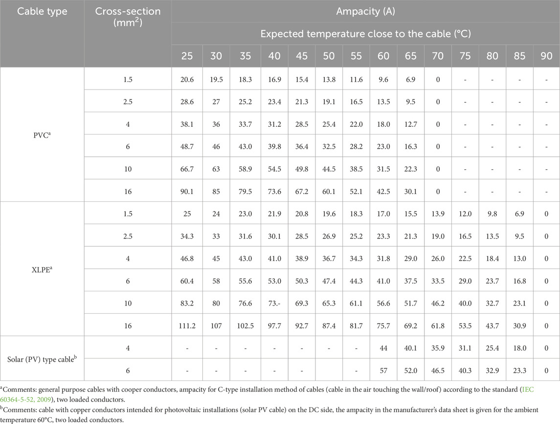
Table 5. Ampacity of cables (for the selected method of laying them) depending on their cross-section and the expected temperature near the cables. Values calculated based on Formulas 4a and 4b.

4 Conclusion

The ampacity of power cables is largely dependent on the ambient temperature. When running cables near PV modules, and especially under them, the cross-section of the cables should be selected very carefully. Advanced numerical studies have shown that the air temperature directly under the PV module can reach 60°C–75°C. This temperature under the PV module/near the cable is achieved when the free air outside the PV system has 25°C. Therefore, it requires the use of cables with appropriate insulation type, as well as correction of the ampacity of the cables in accordance with the expected high temperature in their vicinity. In the area near PV modules, the installation of PVC-insulated cables should be practically excluded, because their continuously permissible temperature is 70°C, and temperatures around PV modules can be at this level (for the worst case scenario). In the case of XLPE-insulated cables the situation is more favourable, but one must remember to correct the ampacity. For example, for a cable with XLPE insulation and a cross-section equal to 6 mm², its ampacity at surrounding air temperature of 75°C is 29.0 A compared to an ampacity of 60.4 A at surrounding air temperature of 25°C. This means a reduction in cable ampacity close to 50%. Considering the very widespread use of PV systems, it seems reasonable to develop tables of the ampacity of cables installed on the roofs of buildings with PV systems, allowing for quick and precise determination of the cable type (mainly the type of insulation) and cable cross-section. In future studies, the authors will consider other PV module arrangements on the building and specific PV installation locations around the world, especially in very warm regions, to calculate temperature around cables in such unfavourable conditions.

The thermal models of the PV system developed by the authors and the numerical studies performed are a step forward towards more accurate calculations of the temperature around PV modules. The results obtained by the authors so far as well as further calculations and subsequent results for other values of PV module power, modules arrangement methods and ambient temperatures can be used when developing amendments to standards for the design of electrical installations related to PV systems.

Data availability statement

The raw data supporting the conclusions of this article will be made available by the authors, without undue reservation.

Author contributions

SC: Conceptualization, Investigation, Methodology, Resources, Supervision, Visualization, Writing–original draft, Writing–review and editing. SS: Investigation, Resources, Software, Writing–original draft, Writing–review and editing. AT: Investigation, Software, Writing–original draft, Writing–review and editing, Visualization. LK: Resources, Visualization, Writing–original draft, Writing–review and editing.

Funding

The author(s) declare that no financial support was received for the research, authorship, and/or publication of this article.

Conflict of interest

The authors declare that the research was conducted in the absence of any commercial or financial relationships that could be construed as a potential conflict of interest.

Publisher’s note

All claims expressed in this article are solely those of the authors and do not necessarily represent those of their affiliated organizations, or those of the publisher, the editors and the reviewers. Any product that may be evaluated in this article, or claim that may be made by its manufacturer, is not guaranteed or endorsed by the publisher.

References

Akbal, B. (2018). OSSB and hybrid methods to prevent cable faults for harmonic containing networks. Elektron. Elektrotech. 24 (2), 31–36. doi:10.5755/j01.eie.24.2.20633

CrossRef Full Text | Google Scholar

Akbal, B. (2019). MSSB to prevent cable termination faults for long high voltage underground cable lines. Elektron. Elektrotech. 25 (6), 8–14. doi:10.5755/j01.eie.25.6.24819

CrossRef Full Text | Google Scholar

Baazzim, M. S., Al-Saud, M. S., and El-Kady, M. A. (2014). Comparison of finite-element and IEC methods for cable thermal analysis under various operating environments. Int. J. Elect. Robot. Electron. Commun. Eng. 8 (3), 470–475.

Google Scholar

Backstrom, R., and Dini, D. A. P. E. (2011). Firefighter safety and photovoltaic installations research project. Northbrook, IL: Underwriters Laboratories Inc. Available at: https://fsri.org/sites/default/files/2021-07/PV-FF_SafetyFinalReport.pdf.

Google Scholar

Bin Wan Mohd Zain, W. A., Ali, N. H. N., Hamdan, M. A., Azis, N., Johari, D., and Rameli, N. (2022). “The effect of the ambient temperature profile in the determination of power cable ratings,” in Presented at the IEEE International Conference on Power System Technology (POWERCON), 12–14 September 2022, Kuala Lumpur, Malaysia.

Google Scholar

Brender, D., and Lindsey, T. (2008). Effect of rooftop exposure in direct sunlight on conduit ambient temperatures. IEEE Trans. Industry Appl. 44 (6), 1872–1878. doi:10.1109/TIA.2008.2006301

CrossRef Full Text | Google Scholar

Cywinski, A., and Chwastek, K. (2021). A multiphysics analysis of coupled electromagnetic-thermal phenomena in cable lines. Energies 14 (7), 2008. doi:10.3390/en14072008

CrossRef Full Text | Google Scholar

Czapp, S., Czapp, M., Szultka, S., and Tomaszewski, A. (2018). Ampacity of power cables exposed to solar radiation–recommendations of standards vs. CFD simulations. E3S Web Conf. 70, 03004. doi:10.1051/e3sconf/20187003004

CrossRef Full Text | Google Scholar

Czapp, S., Szultka, S., and Tomaszewski, A. (2017). “CFD-based evaluation of current-carrying capacity of power cables installed in free air,” in Presented at the 18th International Scientific Conference on Electric Power Engineering (EPE), 17–19 May 2017, Kouty nad Desnou, Czech Republic. doi:10.1109/EPE.2017.7967271

CrossRef Full Text | Google Scholar

de Leon, F. (2006). “Major factors affecting cable ampacity,” in Presented at the IEEE Power Engineering Society General Meeting, 18–22 June 2006, Montreal, QC, Canada. doi:10.1109/PES.2006.1708875

CrossRef Full Text | Google Scholar

Drefke, C., Schedel, M., Balzer, C., Hinrichsen, V., and Sass, I. (2021). Heat dissipation in variable underground power cable beddings: experiences from a real scale field experiment. Energies 14 (21), 7189. doi:10.3390/en14217189

CrossRef Full Text | Google Scholar

EN (2000). Building materials and products–hygrothermal properties–tabulated design values. Report No. EN 12524.

Google Scholar

Enescu, D., Colella, P., and Russo, A. (2020). Thermal assessment of power cables and impacts on cable current rating: an overview. Energies 13 (20), 5319. doi:10.3390/en13205319

CrossRef Full Text | Google Scholar

Falvo, M. C., and Capparella, S. (2015). Safety issues in PV systems: design choices for a secure fault detection and for preventing fire risk. Case Stud. Fire Saf. 3, 1–16. doi:10.1016/j.csfs.2014.11.002

CrossRef Full Text | Google Scholar

Gaitho, F. M., Ndiritu, F. G., Muriithi, P. M., Ngumbu, R. G., and Ngareh, J. K. (2009). Effect of thermal conductivity on the efficiency of single crystal silicon solar cell coated with an anti-reflective thin film. Sol. Energy 83 (8), 1290–1293. doi:10.1016/j.solener.2009.03.003

CrossRef Full Text | Google Scholar

Girshin, S. S., Sorokin, I. A., Smerdin, A. N., Bigun, A. A. Y., Petrova, E. V., Trotsenko, V. M., et al. (2020). Effect of solar radiation on power losses and capacity of insulated and non-insulated wires of overhead power LINES. Przeglad Elektrotechn. 96 (6), 59–63. doi:10.15199/48.2020.06.11

CrossRef Full Text | Google Scholar

Holyk, C., and Anders, G. J. (2015). Power cable rating calculations-A historical perspective [history]. IEEE Ind. Appl. Mag. 21 (4), 6–64. doi:10.1109/MIAS.2015.2417094

CrossRef Full Text | Google Scholar

Hu, Z., Ye, X., Li, Q., Luo, X., Zhao, Y., Zhang, H., et al. (2024). Analysis on three-core power cable temperature field and ampacity model under typical laying environment. Front. Energy Res. 12, 1430501. doi:10.3389/fenrg.2024.1430501

CrossRef Full Text | Google Scholar

IEC (1999). Electric cables–calculation of the current rating (multipart standard). Report No. IEC 60287 (1999, 2023).

Google Scholar

IEC (2009). Low-voltage electrical installations–part 5-52: selection and erection of electrical equipment–wiring systems. Report No. IEC 60364-5-52.

Google Scholar

IEC (2017). Low voltage electrical installations–part 7-712: requirements for special installations or locations–solar photovoltaic (PV) power supply systems. Report No. IEC 60364-7-712.

Google Scholar

Jiang, H., Zhao, X., Liang, Y., and Fu, C. (2023). “Temperature rise and ampacity analysis of buried power cable cores based on electric-magnetic-thermal-moisture transfer coupling calculation,” in Presented at the 13th International Conference on Power and Energy Systems (ICPES), 08–10 December 2023, Chengdu, China.

Google Scholar

Klimenta, D., Perović, B., Klimenta, J., Jevtić, M., Milovanović, M., and Krstić, I. (2018). Modelling the thermal effect of solar radiation on the ampacity of a low voltage underground cable. Int. J. Therm. Sci. 134, 507–516. doi:10.1016/j.ijthermalsci.2018.08.012

CrossRef Full Text | Google Scholar

Musial, E. (2008). Thermal load capacity and overcurrent protection of wires and cables. INPE Inf. Normach Przep. Elektr. 107, 3–41. [in Polish: “Obciążalność cieplna oraz zabezpieczenia nadprądowe przewodów i kabli”].

Google Scholar

Papadopoulos, T. A., Chrysochos, A. I., and Fotos, M. (2023). “Comparison of power cables current rating calculation methods,” in Presented at the 58th International Universities Power Engineering Conference (UPEC), 30 August–01 September 2023, Dublin, Ireland. doi:10.1109/UPEC57427.2023.10294353

CrossRef Full Text | Google Scholar

Perovic, B., Klimenta, D., Jevtic, M., and Milovanovic, M. (2019). A transient thermal model for flat-plate photovoltaic systems and its experimental validation. Elektron. Elektrotech. 25 (2), 40–46. doi:10.5755/j01.eie.25.2.23203

CrossRef Full Text | Google Scholar

PV modules (2024). PV modules–znshinesolar 9BB HALF-CELL bifacial double glass. Available at: https://znshine-solar.pl/ (Accessed August 28, 2024).

Google Scholar

Ruiz-Reina, E., Sidrach-de-Cardona, M., and Piliougine, M. (2014). Heat transfer and working temperature field of a photovoltaic panel under realistic environmental conditions. COMSOL Technical Papers and Presentations. Available at: https://www.comsol.com/paper/heat-transfer-and-working-temperature-field-of-a-photovoltaic-panel-under-realistic-environmental-conditions-18983.

Google Scholar

Sabir, M. D., Khan, L., Hafeez, K., Ullah, Z., and Czapp, S. (2024). Nature-inspired driven deep-AI algorithms for wind speed prediction. IEEE Access 12, 184230–184256. doi:10.1109/ACCESS.2024.3511113

CrossRef Full Text | Google Scholar

Strand, H., Eberg, E., Asklund, K. O., Thomsen, N. M., and Thinn, K. S. (2023). “Experiences with ampacity rating calculations for wind farm export cable,” in Presented at the 27th International Conference on Electricity Distribution (CIRED 2023), 12–15 June 2023, Rome, Italy. doi:10.1049/icp.2023.1201

CrossRef Full Text | Google Scholar

Tommasini, R., Pons, E., Palamara, F., Turturici, C., and Colella, P. (2014). Risk of electrocution during fire suppression activities involving photovoltaic systems. Fire Saf. J. 67, 35–41. doi:10.1016/j.firesaf.2014.05.008

CrossRef Full Text | Google Scholar

Xiong, L., Chen, Y., Jiao, Y., Wang, J., and Hu, X. (2019). Study on the EStudy on the effect of cable group laying mode on temperature field distribution and cable ampacityect of cable group laying mode on temperature field distribution and cable ampacity. Energies 12 (17), 3397. doi:10.3390/en12173397

CrossRef Full Text | Google Scholar

Zenczak, M. (2017). “Approximate relationships for calculation of current-carrying capacity of overhead power transmission lines in different weather conditions,” in Presented at the Progress in Applied Electrical Engineering (PAEE), 25–30, June 2017, Koscielisko, Poland. doi:10.1109/PAEE.2017.8008996

CrossRef Full Text | Google Scholar