Maximizing conventional oil recovery and carbon mitigation: an artificial intelligence-driven assessment and optimization of carbon dioxide enhanced oil recovery with physics-based dimensionless type curves

Introduction: Carbon Dioxide Enhanced Oil Recovery (CO₂-EOR) is a well-established technology that has been deployed for over 2 decades, primarily to boost oil recovery rates. Recently, however, CO₂-EOR has gained attention as a potential carbon mitigation strategy, given its ability to both enhance oil recovery without requiring extensive new drilling and store CO₂ in subsurface formations. This dual function aligns with net-zero carbon goals, as CO₂ is partly trapped in the reservoir through solubility and hysteresis effects on relative permeability. The performance of CO₂-EOR, in terms of both oil recovery and CO₂ storage potential, depends on numerous factors, including reservoir properties such as porosity, permeability, thickness, fluid composition, and operating conditions like bottom-hole pressure and injection rates. Traditional screening for CO₂-EOR candidate reservoirs typically relies on experimental work, simulation studies, and field analogs, all of which require significant time and resources. However, a large dataset exists from prior CO₂-EOR projects, which could enable more efficient screening.

Methods: To leverage this data and capitalize on recent advancements in artificial intelligence, we developed an integrated methodology to predict CO₂-EOR production profiles rapidly and accurately. Using Artificial Neural Networks (ANN), we trained a proxy model (PM) with over 2,000 simulation cases based on real-world CO₂-EOR projects. The model’s novelty lies in its ability to generate dimensionless type curves and their derivatives, which can be matched with production data to estimate average reservoir characteristics at later project stages.

Results and Discussions: Our results demonstrate that the proxy model achieves a high level of accuracy, with a maximum Mean Absolute Error (MAE) of 0.012 and a correlation coefficient of 0.99 between predicted and simulated results across three output variables. Additionally, a sensitivity analysis revealed the significant influence of parameters such as fluid composition, rock-fluid interaction, porosity, permeability, and initial reservoir pressure on CO₂-EOR production profiles. This approach provides a rapid, cost-effective alternative to conventional methods, allowing for quicker and more informed decision-making in CO₂-EOR projects.

1 Introduction

CO₂ flooding, an enhanced oil recovery technique with a history spanning over 4 decades, holds promise for unlocking technically recoverable oil reserves across various global basins (GHG, 2009). Estimates suggest substantial reserves, with the Middle East alone potentially harboring up to 451 billion barrels of technically recoverable oil. In the United States, CO₂ flooding projects yielded around 300,000 barrels per day in 2012 (Dean et al., 2018). Notably, when sourced from industrial emissions (referred to as anthropogenic CO₂), CO₂ used in EOR can have positive environmental implications. By capturing and injecting industrial CO₂ underground, it becomes sequestered within the reservoir, mitigating its atmospheric presence and reducing its contribution to the greenhouse effect. This integration has positioned CO₂ EOR within the framework of Carbon Capture Utilization and Storage (CCUS). In the United States, CO₂ EOR fields have the potential to accommodate between 55 billion to 119 billion metric tons of CO₂ under the “2019 View,” with projected oil production ranging from 84 billion to 181 billion barrels of stranded oil (NPC, 2019).

Various approaches to CO₂-EOR are employed based on specific reservoir conditions and operational constraints. Among these methods, miscible or immiscible flooding stands out as the most prevalent. In miscible flooding, CO₂ is injected at pressures sufficient to achieve full miscibility, effectively blending CO₂ and oil into a single liquid phase. For reservoirs characterized by extensive vertical communication—exhibited by high permeability and continuity of oil-bearing pore space in the vertical direction—a gravity-stabilized miscible flood is often favored as the optimal operational mode, as noted (Claridge, 1972).

Utilizing CO₂ flooding for enhanced oil recovery relies on specific criteria for identifying suitable reservoir candidates. Scholars have put forth various sets of selection criteria over the years. Initially introduced by Taber et al. (1997) (Taber et al., 1997) and subsequently refined by (Aladasani and Bai, 2010), these criteria have been further elucidated by (Yin, 2015) with a focus on US fields. A comprehensive overview of these selection criteria, as outlined by the aforementioned researchers, is presented in Table 1.

Table 1

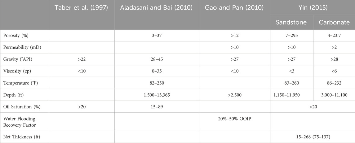
Table 1. CO₂ selection criteria range (Yin, 2015).

In recent years, numerous researchers have explored the application of diverse machine learning algorithms in the design of enhanced oil recovery (EOR) projects, with a particular emphasis on CO₂ flooding strategies. For instance, a deep learning classifier has been employed to forecast the optimal EOR approach by considering multiple factors, including lithology, reservoir characteristics such as depth, porosity, and permeability, as well as reservoir fluid properties like oil gravity and viscosity. Remarkably, this classifier achieved an impressive accuracy level of up to 95% (Kumar Pandey et al., 2023) Additionally, artificial neural network (ANN) algorithms offer a means to investigate the behavior of pure CO₂ foam in porous media and its rheological properties, offering an alternative to labor-intensive laboratory experiments in the context of CO₂ EOR and sequestration endeavors (Iskandarov et al., 2022).

Furthermore, machine learning techniques enable the preliminary evaluation of CO₂ storage in residual oil zone reservoirs under various scenarios, such as continuous CO₂ injection or WAG (water alternating gas), aiding in the determination of CO₂ storage capacity. Notably, the Multivariate Adaptive Regression Splines (MARS) technique has demonstrated superior accuracy in this context (Chen and Pawar, 2019).

Proxy models serve as efficient tools that swiftly provide insights typically derived from extensive simulation studies. These models are based on predefined parameter equations and leverage hybrid machine learning algorithms such as least squares support vector machines (LSSVM) and box-Behnken design (BBD) to generate predictions, notably exhibiting satisfactory results in forecasting oil recovery factors in CO₂ injection scenarios (Ahmadi et al., 2018).

Carbon dioxide is recognized as one of the greenhouse gas emissions (GHG). Reports indicate that between 2006 and 2015, approximately 38 giga metric tons per year of CO₂ were discharged into the atmosphere from anthropogenic sources, encompassing activities such as fossil fuel emissions and land-use changes. Despite the capacity of ocean and terrestrial plants to act as sinks for CO₂, thereby reducing its atmospheric concentration, the rate of emissions surpasses the sink’s capacity, resulting in an annual accumulation of CO₂ in the atmosphere at a rate of 2 parts per million (ppm) (Le Quéré et al., 2016). Globally, nations have committed to attaining carbon emission neutrality, with 90% of them targeting 2050 as the deadline for this objective, while others aim for 2060. Carbon Capture, Utilization, and Storage (CCUS) emerges as a climate change mitigation strategy, involving the capture of emitted CO₂ from stationary sources and subsequent distribution for either utilization or storage purposes (Tapia et al., 2018). Geological storage of CO₂ in subsurface formations represents a viable pathway towards achieving net zero emissions goals. Such storage can take various forms, including injection into saline aquifers, depleted oil reservoirs, or CO₂-EOR projects. Given that only a fraction (50%–67%) of injected CO₂ in EOR projects is recoverable at the surface alongside produced oil, the remainder is sequestered in the subsurface (Orr, 2018). CO₂-EOR projects exhibit 37% lower emissions per barrel compared to other production methods (Novak Mavar et al., 2021). Unlike other underground CO₂ storage projects, CO₂ EOR projects are economically advantageous as they enhance oil production, which can be monetized for a net profit, while other injection projects rely solely on government-provided tax reduction incentives (Novak Mavar et al., 2021). An essential performance metric for evaluating the success of CO₂ storage in CO₂ EOR is the estimation of the CO₂ Retention Factor, defined as:

$C{O}_{2}Retention\%=\frac{C{O}_{2}RemainingatSubsurface}{CummulativeC{O}_{2}Injected}\times 100(1)$

In CO₂-EOR projects across the United States, retention factors vary between 28% and 98.7% for both continuous and WAG injection methods, contingent upon reservoir parameters, lithology, and the volume of hydrocarbon pore volume injected (HCPVI). In miscible CO₂ flooding endeavors, an increase in the injected CO₂ HCPVI correlates with a reduction in the retention factor (Olea, 2015).

In this research, an initial compositional simulation model served as the foundation. Eight synthetic fluid composition templates and nine synthetic relative permeability templates were developed, encompassing a wide spectrum of data found in the literature Figures 1, 2. Additionally, ranges for reservoir properties such as porosity, permeability, and initial reservoir pressure were defined based on published CO₂-EOR projects. Then using Latin hypercube sampling generated more than 2000 simulation cases. The simulation results dataset is used to build the proxy model which is then used to predict the results and generate dimensionless type curves. The workflow of the research is shown in Figure 3.

Figure 1

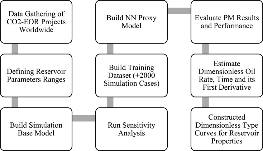
Figure 1. Phase envelope of PVT templates.

Figure 2

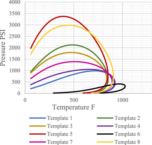
Figure 2. Water-oil relative permeability templates.

Figure 3

Figure 3. Water-oil relative permeability templates.

2 Numerical reservoir simulation

The investigation utilized the tNavigator Compositional module, a commercial software package. The fundamental equation dictating flow within porous media is the Mass Conservation equation for each component, as outlined by (Chen et al., 2006) in Equation 2:

$\frac{\partial }{\partial t}\left(\varnothing c_i^{\sim }{\rho }_i\right)=-\nabla .\left({\displaystyle \sum _{\alpha =1}^{N_p}}{\rho }_i\left[c_{i\alpha }{u}_{\alpha }-D_{i\alpha }\nabla c_{i\alpha }\right]\right)+q_{i}i=1,2,\dots \dots \dots N_c(2)$

where:

$c_i^{\sim }$ are the overall concentration phases, $N_p$ is the number of phases, ${\rho }_i$ mass density, $q_i$ is source/sink term, $c_{i\alpha }$ and $D_{i\alpha }$ are concentration and diffusion-dispersion tensor of component $i$ in phase $\alpha$.

The base model comprises a box configuration encompassing 64,000 cells, all possessing identical vertical and horizontal permeability within the reservoir. Porosity remains constant at a single value as specified in Table 2. This model features two wells: one functioning as a producer and the other as an injector. The controlling mode for both is the Bottom hole Pressure. Injection operations lasted for 30 years commenced on day 1 to uphold pressure levels, with the bottom hole flowing pressure (BHFP) limit set 1,470 psi to be higher than both the minimum miscibility pressure (MMP) and the bubble point pressure, ensuring single-phase flow within the reservoir and the bottom hole injection pressure set to be 6,000 psi to ensure that it does not exceed fracture pressure. The maximum production rate was set to be 5000 STB/D and maximum injection rate is 10,000 MSCF/D. Initial conditions were established within the oil production zone, devoid of free water or gas, situated above the oil-water contact, and below the gas-oil contact Table 2. Using template one of the defined fluid composition and relative permeability templates.

Table 2

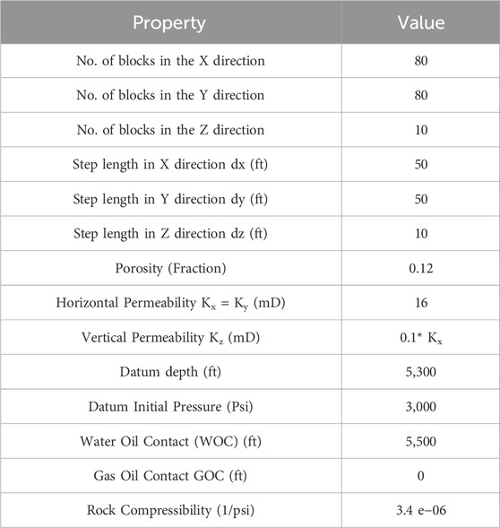
Table 2. Base model description.

3 Dimensionless curves

Drawing upon the pioneering work of (Arps, 1945) in decline curve analysis, the normalization of rates based on post-flow rates has been applied in multiphase flow analysis as introduced by (Fetkovich and Vienot, 1984), alongside other type-curves for various assessments (Doublet and Blasingame, 1995). Blasingame further delved into decline curve analysis in the context of secondary recovery scenarios involving water influx and waterflood cases. In the present study, we computed dimensionless oil rate using Equation 3 and time using Equation 4, along with their first derivative, serving as a diagnostic tool for reservoir properties. The definition of dimensionless numbers aligns with that employed by (Fetkovich, 1973).

3.1 Dimensionless rate

$q_D=\frac{141.2\times q\times \mu \times \beta }{K\times h\times \left(P_i-BHFP\right)}\times \frac{L}{W}(3)$

3.2 Dimensionless time

$t_D=\frac{0.00634\times K\times t}{\varnothing \times \mu \times C_t\times r_w^2}(4)$

Where $q$ is the production oil flow rate in STB/day, $\mu$ is the oil viscosity in cp, $\beta$ is the oil formation volume factor in bbl/STB, $K$ is the reservoir permeability, $h$ is the reservoir thickness, $P_i$ is the reservoir initial pressure in Psi, $BHFP$ is the bottom hole flowing pressure in Psi, $\varnothing$ is the reservoir porosity, $C_t$ is the total compressibility in 1/psi, $r_w$ is the wellbore radius.

Calculating the first derivative of the dimensionless oil flow rate using the Bourdet method as shown in Equation 5 (Bourdet et al., 1989):

${dQ}_d=\frac{\left(\frac{∆{Qd}_1}{∆{Dt}_1}∆{Dt}_2+\frac{∆{Qd}_2}{∆{Dt}_2}∆{Dt}_1\right)}{∆{Dt}_1+∆{Dt}_2}(5)$

Where, $∆{Qd}_1$ is the change of dimensionless oil rate, $∆{Dt}_1$ is the change of dimensionless time, 1 and 2 are at two consecutive points.

We noted several recurring patterns within the generated dimensionless curves:.

1. In the later stages of production, three distinct regions emerge, as illustrated in Figure 4:

⁃ Pre-decline: Initial stable production occurs at the maximum allowable rate; preceding water or gas breakthrough, the slope is nearly flat.

⁃ Decline: The onset of oil rate decline is marked by a trough in the first derivative; alterations in reservoir and operational parameters affect the width, depth, location of the trough, and steepness of the slope on the curves.

⁃ Post-Decline: Once the production rate nears its minimum value, minimal changes occur, resulting in the first derivative slope being nearly flat.

2. The alteration in slope within the trough area is influenced by changes in oil rate, gas rate, and water rate profiles. Typically, following breakthrough, the gas rate continues to rise, whereas the water rate increases initially before declining thereafter. This transition often yields a secondary shallower trough as depicted in Figures 5, 6.

3. The derived slopes pertain to the late-time production trough. We specifically identified four slopes to capture variations, though additional definitions are possible. The extent of the trough vertically is governed by the lowest point in the curvature, while its width encompasses both primary and secondary troughs, estimated as the entire region between two zero slopes, as depicted in Figure 4.

Figure 4

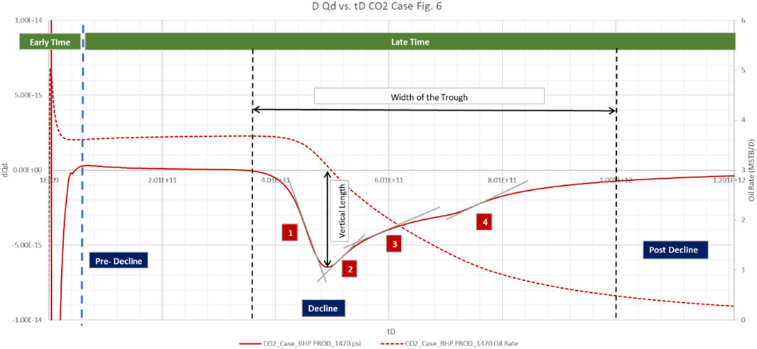
Figure 4. First derivative of dimensionless oil rate and oil rate versus dimensionless time (trough description).

Figure 5

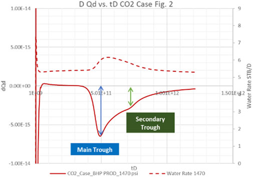
Figure 5. First derivative of dimensionless oil rate and water rate versus dimensionless time.

Figure 6

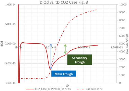
Figure 6. First derivative of dihmensionless oil rate and gas rate versus dimensionless time.

4 Parameters’ sensitivity

In this segment, a sensitivity analysis was performed on the base model, where one parameter was altered at a time while keeping all other reservoir variables constant. This aimed to assess their influence on production. We examined the repercussions of modifying reservoir properties in specific range, including fluid composition on 8 templates, rock-fluid interaction on 9 templates, porosity in the range of 0.05 and 0.385, permeability in the range of 2 and 980 mD, and initial pressure in the range of 1,500 psi and 5,000 psi, alongside operational factors like the bottomhole flowing pressure of the producer well in the range of 1,470 psi and 4,764 psi. Diagnostic plots employed for comparison encompassed dimensionless type curves, oil recovery factor, and CO₂ retention factor plotted against the hydrocarbon pore volume injected, as well as oil, gas, and CO₂ molar production rates.

4.1 Fluid composition sensitivity

The recovery efficiency of CO₂ flooding EOR is influenced by the composition of the oil. Optimal displacement efficiency is attained at a minimal miscibility pressure, which correlates inversely with the weight percentage of hydrocarbons ranging from C5 to C30 (Holm and Josendal, 1982). The presence of light components such as C2 to C4 in reservoir oil does not significantly affect the recovery process, as these gases tend to channel and bypass the miscible bank. However, the inclusion of methane (C1) in reservoir oil diminishes the overall recovery efficiency (Holm and Josendal, 1974).

The suggested scope for employing CO₂ miscible flooding in oil reservoirs is for those with an API gravity exceeding 30. As the gravity of reservoir oil rises, its viscosity diminishes, leading to a more advantageous mobility ratio and improved sweeping efficiency. Additionally, with increasing oil gravity, there is a greater presence of intermediate components (C5-C20) which undergo condensation or vaporization processes necessary for achieving miscibility (Klins, 1984). Factors such as reservoir temperature, critical properties, and bubble point pressure influence the minimum miscibility pressure attained (Holm and Josendal, 1982).

Data extracted from literature on prominent CO₂ flooding projects revealed a variation in oil density ranging from 25 to 45 API, with prevalent values, concentrated within the 35 to 40 API range. Reservoir temperatures spanned from a minimum of 83°F to a maximum of 267°F, while bubble point pressures exhibited a range of 300–2200 PSI. Minimum Miscibility Pressure values were observed to fluctuate between 900 and 4500 PSI, with the majority clustering within the 1,100 to 2,500 PSI range.

Subsequently, after compiling fluid composition data from 14 significant CO₂ flooding sites, eight templates were generated to represent the characteristics found in the literature. These templates were then utilized in constructing simulation scenarios, as depicted in Table 1 in supplemental material. The templates cover a range of oil density from 21 to 109 API, bubble point pressures spanning 103 to 2625 PSI, and MMP ranging from 1,090 to 3,460 PSI.

The employed PVT templates vary in composition and reservoir temperatures, resulting in varied behaviors regarding oil recovery and storage capacity were shown in Figure 7. Under consistent conditions, we observed that Template_7 yielded the highest initial oil rate, with a corresponding decrease in the initial oil rate anticipated as the oil’s API gravity diminishes.

Figure 7

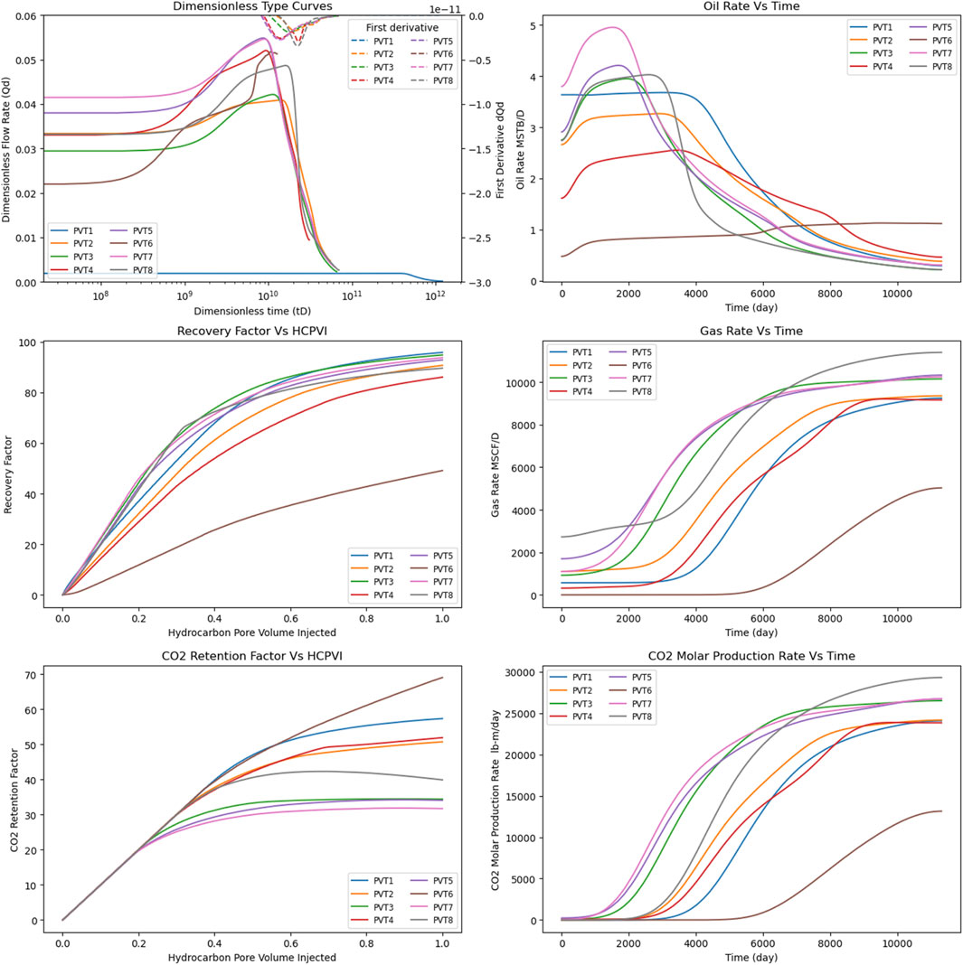
Figure 7. PVT Templates Sensitivity Analysis, starting from the top left is Dimensionless Rate and its first Derivative vs dimensionless time, Recovery Factor vs standard HCPVI, CO₂ Retention Factor Vs HCPVI, Oil Rate, Gas Rate, and CO₂ Production Moles Vs Time.

Template_8 and Template_3 exhibited deviations from this pattern owing to additional characteristics influencing their performance. Despite Template_8 having the highest API gravity, which typically implies the highest recovery, its oil composition features a notably high percentage of C1, elevating the bubble point pressure to 2,625 psi. Given that the set bottom hole flowing pressure is approximately 1,470 psi, lower than the bubble point, some oil molecules may have vaporized into gas, thereby augmenting the gas-oil ratio at the expense of oil rate production.

Template_3, despite having a lower API value compared to Template_2 and Template_1, exhibited a higher initial oil rate. This outcome may be attributed to its higher percentage of intermediate components (C5-C20), which are conducive to the multiple evaporation and condensation processes essential for miscible recovery. In terms of recovery factor, while Template_1 did not attain the highest initial oil rate, its production decline occurred later, enabling the accumulation of a greater cumulative oil total and consequently, the highest recovery factor. Conversely, Template_6, characterized by the highest C21+ component, yielded the lowest recovery factors. CO₂ retention factors varied among templates; Template_6 achieved the highest CO₂ retention factor, with the template featuring the lowest C1 content exhibiting the lowest gas production. Template_7 recorded the lowest CO₂ retention.

Among the dimensionless oil rates, Template_7 exhibits the highest value, reflecting its superior oil rate. Meanwhile, Template_8 displays the deepest trough in the first derivative of the oil rate.

4.2 Relative permeability sensitivity

Given that fluid flow within porous media involves multiple phases—oil, gas, and water—alongside CO₂ displacement of oil and water in CO₂ flooding scenarios, either immiscible or miscible, where CO₂ and oil blend into a single non-wetting phase, the saturation of each phase fluctuates during production initiation. Thus, relative permeability curves are indispensable for elucidating the effective permeability of each phase. Various factors influence the behavior of relative permeability curves, including rock composition, wettability, pore size distribution, interfacial tension, and phase viscosity. Relative permeability curves were compiled from literature sources of common fields and categorized into templates based on rock type, viscosity ratio (oil to water), and interfacial tension. Twenty-one samples of relative permeability curves from reservoir fields were utilized, undergoing smoothing via Corey correlation. The parameters of the Corey Correlation of the 9 templates are presented in the Supplementary Table S2.

Under constant parameters, modifications to the utilized relative permeability curve templates lead to alterations in production behavior as shown in Figure 8. Template_6 demonstrates the highest oil production rate and dimensionless rate among all templates. Conversely, Template_4 exhibits the lowest production rates, attributed to its highest capillary pressure among the templates, a characteristic reflected in its elevated CO₂ retention factor. In contrast, Template_7, characterized by the lowest capillary pressure, facilitates earlier gas and CO₂ breakthroughs, resulting in a lower CO₂ retention factor. The influence of capillary pressure is further evidenced in the derivative of the dimensionless oil rate, with Template_7 showing the deepest trough, indicating a rapid rate of decline, while Template_4 exhibits the shallowest trough, indicative of its high capillary pressure.

Figure 8

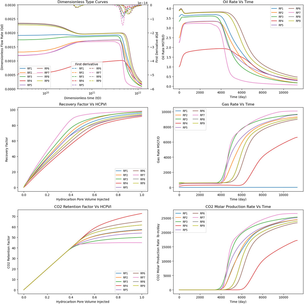
Figure 8. RP Templates Sensitivity Analysis, starting from the top left is Dimensionless Rate and its first Derivative vs dimensionless time, Recovery Factor vs standard HCPVI, CO₂ Retention Factor Vs HCPVI, Oil Rate, Gas Rate, and CO₂ Production Moles.

4.3 Porosity sensitivity

As porosity increases, the dimensionless oil rate also increases, albeit with a quicker initial decline, resulting in a deeper trough. However, production subsequently, stabilizes for an extended duration, potentially without experiencing a secondary trough observed in other cases. Conversely, gas and CO₂ molar production rates rise with decreasing porosity, leading to a decrease in the CO₂ retention factor. The results for the sensitivity of porosity are shown in Figure 9.

Figure 9

Figure 9. Porosity Sensitivity Analysis, starting from the top left is Dimensionless Rate and its first Derivative vs dimensionless time, Recovery Factor vs standard HCPVI, CO₂ Retention Factor Vs HCPVI, Oil Rate, Gas Rate, and CO₂ Production Moles Vs Time.

4.4 Permeability sensitivity

As permeability decreases, the oil rate increases, albeit with a swifter decline due to the ease of gas breakthrough, consequently diminishing the ultimate oil recovery factor. The dimensionless oil rate demonstrates an increase, accompanied by an earlier onset of the decline stage and a shallower trough in the first derivative. The optimal oil recovery factor is observed at moderate permeability values around 50 mD. While high permeability values enhance oil flow, they accelerate water and gas breakthroughs, thereby reducing recovery. Conversely, lower permeability yields better values for CO₂ retention, attributed to enhanced CO₂ storage resulting from solubility. The results for the sensitivity of permeability are shown in Figure 10.

Figure 10

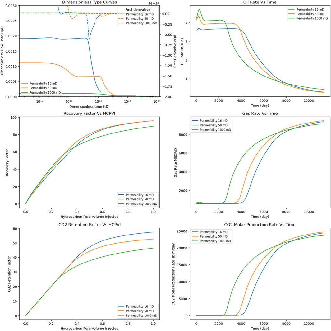
Figure 10. Permeability Sensitivity Analysis, starting from the top left is Dimensionless Rate and its first Derivative vs dimensionless time, Recovery Factor vs standard HCPVI, CO₂ Retention Factor Vs HCPVI, Oil Rate, Gas Rate, and CO₂ Production Moles Vs Time.

4.5 Initial reservoir pressure sensitivity

The initial pressure must exceed the BHFP to ensure adequate drawdown. A higher initial pressure results in a prolonged period of stabilized rate initially, yet thereafter, its influence on oil recovery, gas, or CO₂ production diminishes. However, distinctions can be noticed in the dimensionless rate and its first derivative with varying initial pressures. As the initial pressure rises, the dimensionless rate decreases, and its first derivative exhibits a deeper trough. The results for the sensitivity of initial reservoir pressure are shown in Figure 11.

Figure 11

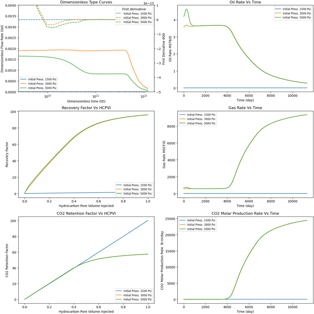
Figure 11. Initial Reservoir Pressure Sensitivity Analysis, starting from the top left is Dimensionless Rate and its first Derivative vs dimensionless time, Recovery Factor vs standard HCPVI, CO₂ Retention Factor Vs HCPVI, Oil Rate, Gas Rate, and CO₂ Production M.

4.6 Bottom hole flowing pressure sensitivity

When the Bottom Hole Flowing Pressure (BHFP) remains higher than the Minimum Miscibility Pressure (MMP), an increase in the BHFP of the producer well corresponds to an increase in the dimensionless oil rate, along with a shallower trough in its derivative. Although the oil rate decreases, it takes slightly longer to enter the decline phase. Meanwhile, gas and CO₂ molar production decreases, leading to an improvement in the CO₂ retention factor. The results for the sensitivity of bottom hole flowing pressure are shown in Figure 12.

Figure 12

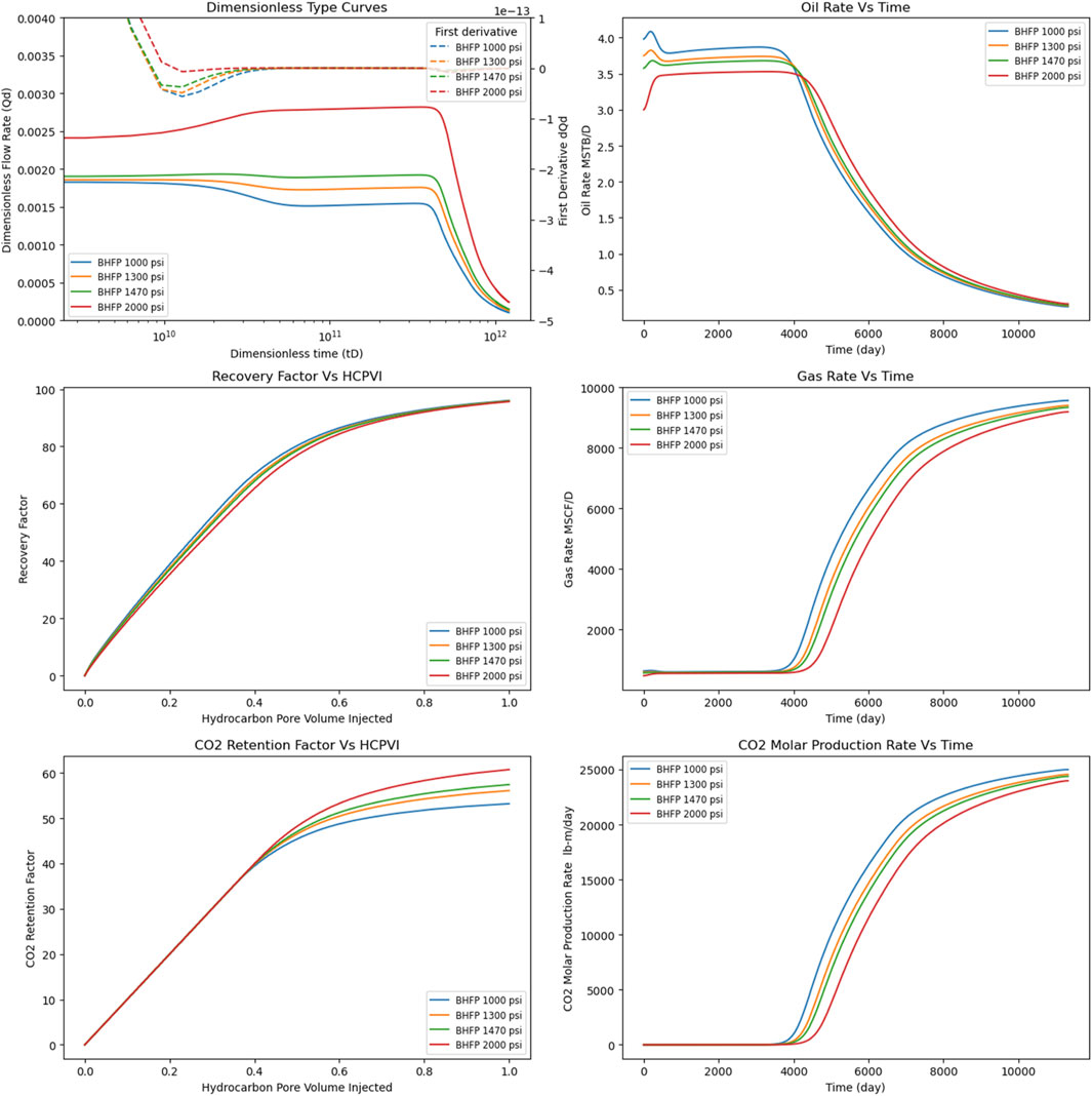
Figure 12. Bottom Hole Flowing Pressure Sensitivity Analysis, starting from the top left is Dimensionless Rate and its first Derivative vs dimensionless time, Recovery Factor vs standard HCPVI, CO₂ Retention Factor Vs HCPVI, Oil Rate, Gas Rate, and CO₂ Production Molar Rate Vs Time.

5 Dataset development

Our aim in this stage is to acquire a dataset that accurately represents the reservoir field data of the CO₂ EOR application, which will serve as the training data for the machine learning model. To achieve this, we employed the compositional box model utilized in the sensitivity analysis as the foundational model for simulation work, utilizing tNavigator reservoir simulation software modules to generate the requisite data. To encompass a wide range of conditions, we conducted experiments in two phases. The variable parameters were selected based on the common selection criteria for CO₂-EOR projects found in the literature, as shown in Table 1, with some modifications to suit our approach. Instead of defining reservoir fluid properties such as viscosity, API, and MMP directly, we used predefined PVT templates. Similarly, instead of relying on saturation and different rock types, we employed various relative permeability templates to represent these properties.

Initially, we developed base models with varying reservoir fluid properties and relative permeability, resulting in the creation of 8 reservoir fluid composition templates and 9 relative permeability templates. These templates were constructed based on field data obtained from the literature. By combining each PVT template with each relative permeability template, we generated a total of 72 base model cases. Throughout these base cases, porosity, permeability, and initial pressure remained constant.

In the second phase, we varied the porosity, permeability, and initial pressure for each of the 72 base models. We employed the Assisted History Matching (AHM) module to conduct a Latin hypercube experiment for each case, running 30 model iterations per case. This process yielded a total of 2,160 models after filtering out cases with errors.

The Latin Hyper Cube algorithm operates by generating model variations according to the user-specified number of variants, denoted as N, and the number of variables, denoted as M. It partitions the search space into N hyperplanes, with each hyperplane containing precisely one variant. This method aids in covering a wide range of possibilities within the search space (McKay, 1992).

Each of the 72 cases served as a base scenario, from which 30 sensitivity cases were derived by adjusting the porosity, permeability, and initial reservoir pressure. To ensure comprehensive coverage, we employed the Latin hypercube experiment. The parameter ranges were determined based on literature data, with distributions chosen to ensure representative coverage. For instance, a truncated normal distribution was utilized for permeability to predominantly reflect lower values observed in the literature. The ranges for porosity and permeability remained consistent across all cases, while the range for initial reservoir pressure varied with changes in PVT templates to ensure the initial value exceeded the bottomhole flowing pressure of the producer well, set above the MMP. The maximum oil rate was capped at 5000 STB/D, the gas injection rate at 10,000 MSCF/D, and the bottomhole injection pressure limit at 6000 PSI to encompass a broad spectrum of scenarios.

The input ranges for porosity, permeability, and initial pressure were compared to the ranges observed in field cases gathered from literature sources as shown in Figure 13. Analysis of the scatter plot reveals that porosity exhibits a linear distribution encompassing the full range of field data. Permeability distribution predominantly clusters within the 0–200 mD range, with fewer cases observed beyond this range. Conversely, the distribution of initial pressure covers the entire field data range, with a notable concentration of cases at higher values exceeding 2500 PSI. This concentration aligns with expectations, as the input values were deliberately selected to surpass the Minimum Miscibility Pressure (MMP).

Figure 13

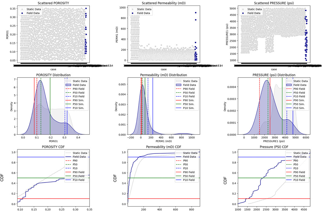
Figure 13. Pre-Simulation Input Values Distributions compared with the Field Data for Porosity, Permeability, and Initial Reservoir Pressure.

The post-simulation analysis revealed that the simulated data spans the spectrum of recovery factors and hydrocarbon pore volume injected observed in field operations. However, the P50 recovery factor derived from simulation data appears more optimistic compared to field data. This disparity can be attributed to the fact that injection in simulation scenarios commenced from day 1, facilitating pressure maintenance and resulting in higher recovery rates. In contrast, much of the recovery data reported in the literature pertains to secondary or tertiary recovery, indicating incremental gains, which consequently exhibit lower values compared to simulations, although simulation data spans the entire range, the P50 value is notably higher in simulations, as illustrated in Figure 14.

Figure 14

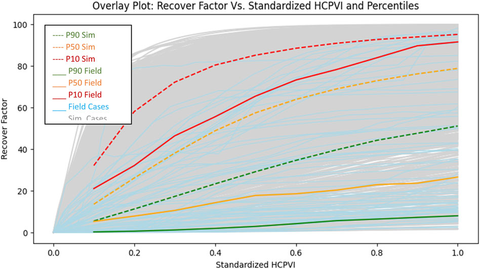
Figure 14. Recovery factor versus standardized hydrocarbon pore-volume injected simulation results compared with field data.

6 Proxy model development

Proxy models are constructed by leveraging established models with reliable outcomes, wherein parameters deemed influential are selected for a fitting process. This process estimates results for additional cases if input values fall within the parameter range used to construct the proxy model (Bahrami et al., 2022). Artificial Neural Networks (ANNs) draw inspiration from the functioning of biological neurons in the human brain. The network comprises an input layer representing input parameters, an output layer indicating the target parameter to be predicted, and multiple hidden layers in between. Neurons within each layer are computed based on preceding layer neurons, weights, and a bias factor (Mohaghegh, 2000). In our study, ANN was employed to develop a proxy model for predicting oil flow rate (Qo), gas rate (Qg), and CO₂ production. Optimal fit and accurate predictions were achieved through testing various configurations of neurons and layers. Input parameters were categorized into reservoir parameters, such as initial reservoir pressure, porosity, permeability, relative permeability templates, and PVT/fluid composition templates, and operational parameters, including gas injection rate, bottomhole injection pressure, and bottomhole flowing pressure. The ranges of input data are detailed in Table 3:

Table 3

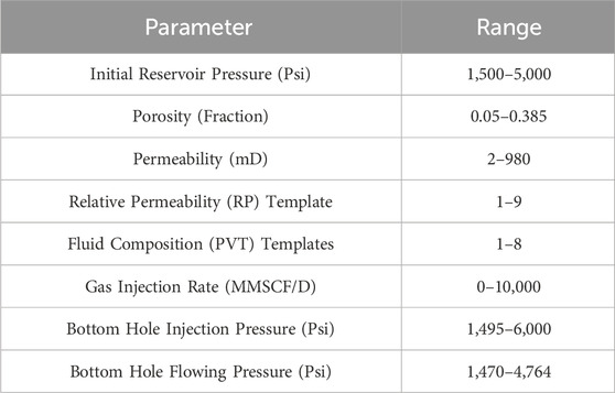
Table 3. Proxy model input data range.

To ensure uniformity in input data scales and prioritize parameters equally in the model’s initial impact, datastandardization was executed. This process was guided by the mathematical expression outlined by Equation 6 (Muther et al., 2021):

$x_{standard}=\frac{x-Mean}{StandardDeviation}(6)$

Where x is the value of each parameter in the input or output data.

To assess the impact of each input parameter on the target output parameter, we employed the Random Forest Regressor method. This approach involves partitioning the data into subsets and evaluating the variance reduction for each attribute at every tree level (Ho, 1995, p. 1). This technique is utilized to determine the importance of input parameters, irrespective of whether they contribute to an increase or decrease in the output (Belyadi and Haghighat, 2021).

It’s observed in Figure 15 that time holds the most significant influence on production, as anticipated, followed by porosity. Conversely, initial pressure exhibits the least impact on production, as anticipated, given that once CO₂ injection commences, it can surpass initial pressure values and exert a greater influence.

Figure 15

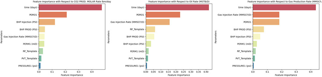
Figure 15. Feature Ranking of the input parameters for the predicted output using Random Forest Regressor.

The dataset is divided into an 80% portion for training the model and adjusting weights, while the remaining 20% is further divided into two equal parts: 50% serves as a testing dataset for evaluating prediction accuracy, and the remaining 50% acts as a validation set to assess model performance. Additionally, we employ 10-fold cross-validation by default during the splitting process to minimize the risk of overfitting and ensure robust model evaluation. As previously discussed, the model’s architecture comprises layers and nodes, with each node’s calculation based on preceding layer nodes, their weights, and a bias factor. An activation function is employed to constrain each node’s output value within the range of 0–1, aiding in capturing nonlinear relationships between nodes. The Rectified Linear Unit (ReLU) activation function was utilized in this study. Optimization algorithms are used to improve the accuracy and robustness of searching for the optimum weight factors for achieving the minimum objective function by adjusting the learning rate. The algorithm we used is ‘Adam’, which is suitable for large dataset problems; it is based on adjusting lower-order moments (Kingma and Ba, 2017).

The neural network model aims to determine optimal weights that minimize the objective function. In the case of a regression neural network, this objective function can be one of several regression evaluation metrics, such as mean absolute error (MAE), mean squared error (MSE), and root mean squared error (RMSE). In our model generation process, we utilized MAE as the objective function, while employing other metrics for model evaluation. MAE computes the average absolute difference between actual and predicted values, expressed by the formula (Belyadi and Haghighat, 2021) where $n$ represents the number of sample points, $y_i$ denotes the actual output, and $y_i$ represents the predicted output from the model as shown in Equation 7:

$\frac{1}{n}{\displaystyle \sum _{i=1}^n}\left|y_i-\stackrel{`}{y_i}\right|(7)$

The evaluation of the proxy model involved several stages. The initial stage involved plotting the loss function against the trained epoch numbers. Ideally, as the ANN model undergoes training, the loss function should diminish with increasing epoch numbers. A well-trained model is expected to exhibit decreasing loss values for both the training and testing datasets, as depicted in Figure 16 for the three outputs of the proxy model.

Figure 16

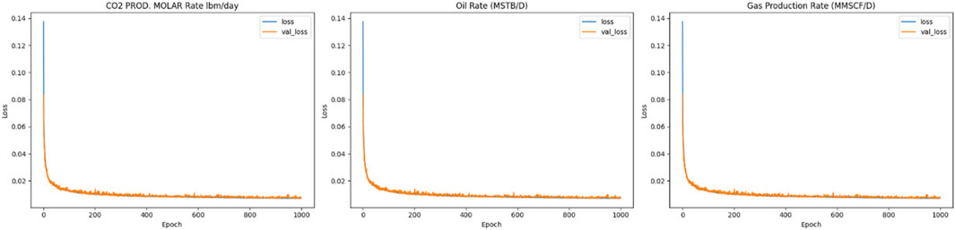
Figure 16. Training and testing losses for CO₂ production molar rate, oil rate, and gas production rate.

The second evaluation stage involves creating a cross-plot to compare the actual simulation results with the predictions from the trained neural network (NN) model, both presented in their standardized form. This plot demonstrates a strong correlation, as illustrated in Figure 17. Although some data points may appear scattered, the overall results are consistent and satisfactory.

Figure 17

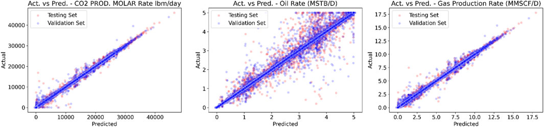
Figure 17. Actual Data vs ANN Predicted Data for the Testing and Validation datasets of CO₂ Production Molar Rate, Oil Rate, and Gas Rate.

Another evaluation stage was establishing the performance metrics, which quantify the variance between the predicted outcomes from the proxy model and the actual results from the simulation. These metrics, shown in Table 4, reveal positive outcomes, demonstrating an acceptable level of accuracy across all three outputs.

Table 4

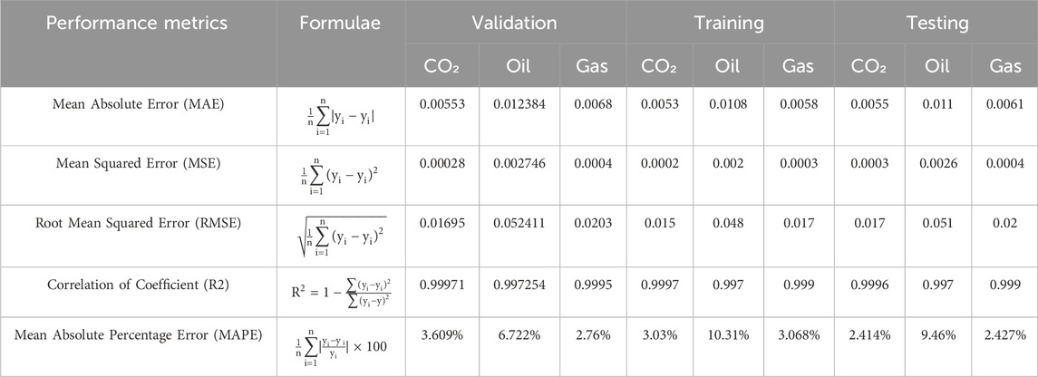
Table 4. Performance metrics between actual and proxy model outputs.

The final evaluation checkpoint involves plotting individual cases. It was observed that the majority of cases exhibit a precise alignment. One interesting observation demonstrating the robustness of the training and testing process to ensure the generalization capability of the trained proxy models without memorization or overtraining is their insensitivity to noise. We deliberately included the results of some cases, as illustrated in Figure 18, where oscillations in the simulation results are observed due to convergence during numerical simulation. However, the trained proxy model did not incorporate these oscillations and noise but instead accurately captured the simulation’s underlying physical trend.

Figure 18

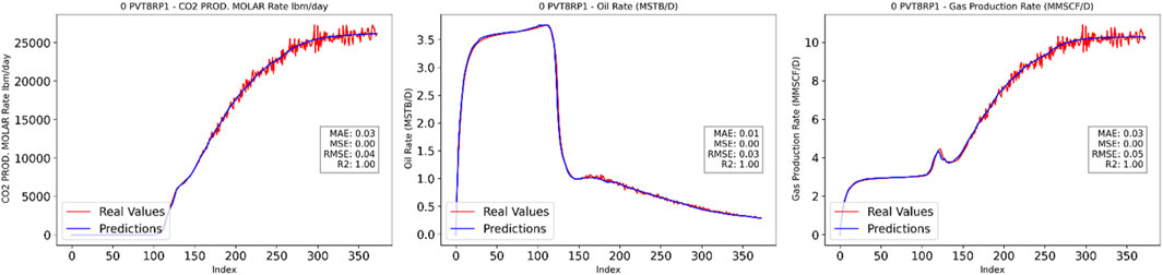
Figure 18. Real and Predicted Results for case PVT8RP1 Base Case, for CO₂ Production Molar Rate, Oil Rate, and Gas Production Rate.

7 Screening and designing applications

The utilization of the trained ANN proxy model depends on the phase of the CO₂ project under consideration. In the initial design stage, where data availability is limited, primarily sourced from analog or neighboring fields, numerous uncertainties arise. During this phase, the aim of employing the proxy model is to swiftly assess the spectrum of outcomes for various scenarios and their economic feasibility.

Imagine a fresh field where we’re aiming to introduce CO₂ EOR. The uncertainties we confront are having two different possiple fluid composition templates; template 1 or 8, three different relative permeability templates; template 1, 2 or 3, three porosity values 0.06, 0.12 or 0.16, and three permeability values 8 mD, 16 mD or 32 mD. Employing the ANN Proxy model allows us to generate diverse scenarios that tackle these uncertainties. Consequently, we can obtain approximations of the highest, median, and lowest production profiles, illustrated in Figure 19. These profiles serve as inputs for conducting techno-economic analyses. Furthermore, the proxy model can be used to predict the amount of produced CO₂ in moles. By combining this with the injected CO₂ moles, the CO₂ retention factor can be estimated using Equation 1.

Figure 19

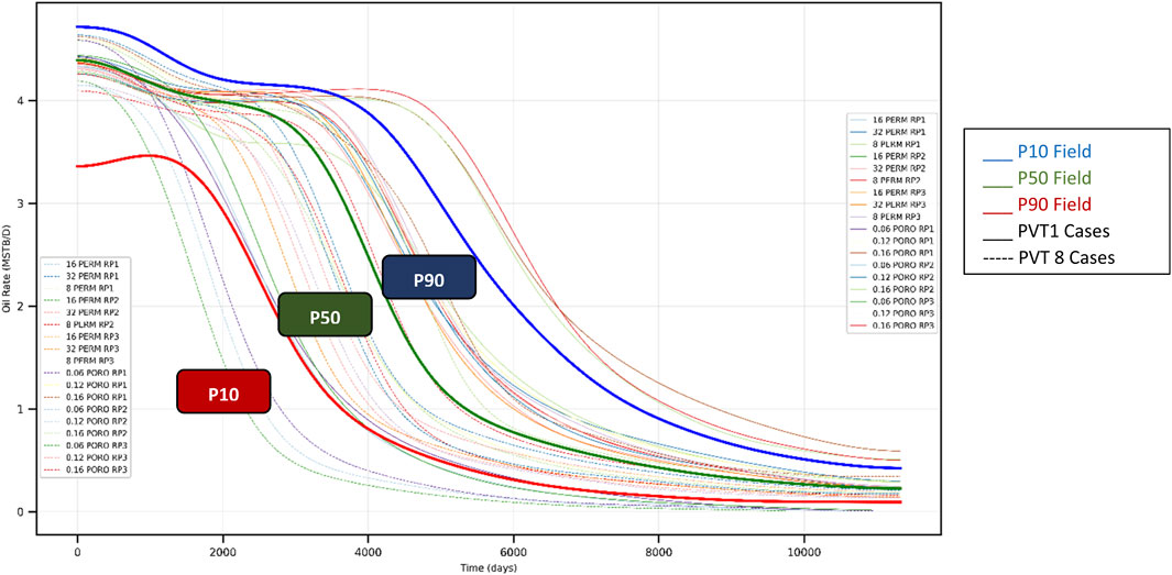
Figure 19. Oil flow rate (mstb/d) vs Time (days) of pre-pilot example with uncertainties.

8 Post-pilot application

The ANN Proxy model was utilized to create type curves representing the dimensionless oil rate (Qd) and its first derivative against dimensionless time (tD). This involved employing 8 fluid composition templates and 9 relative permeability templates while adjusting porosity, permeability, and initial pressure. As we transition into the post-pilot stage, where data collection begins and production profiles emerge, these dimensionless type curves serve to refine the remaining missed reservoir data. For instance, suppose the pilot well operation yields a production profile akin to the dotted plot depicted in Figure 20. By aligning this profile with the type curves generated by the proxy model, we can infer its resemblance to a scenario characterized by the fluid composition of template 1, relative permeability curves of template 2, a permeability of 16 mD, porosity of 0.12, and an initial pressure of 3000 PSI Figure 21. Importantly, this method extends beyond the values illustrated in the type curves; interpolated values can also be derived using the same proxy model, thereby enhancing its applicability across a broader spectrum of scenarios.

Figure 20

Figure 20. Dimensionless Oil Rate and its First Derivative vs Dimensionless Time for Post-Production Application Pilot Data Example.

Figure 21

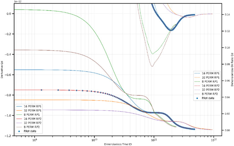
Figure 21. Dimensionless Oil Rate and its First Derivative vs Dimensionless Time for Post-Production Application Example After Matching.

9 Summary and conclusion

In summary, various reservoir characteristics significantly influence the production behavior of both CO₂-EOR projects and CO₂ storage endeavors. Advancements in machine learning can support both design and implementation phases. Key findings from this study include:

⁃ Sensitivity analysis indicates that while some properties, such as initial reservoir pressure, have a slightly lesser impact on production profiles, dimensionless type curves provide a distinctive response that characterizes reservoir behavior effectively.

⁃ The proposed ANN-based proxy model (PM) offers a computationally efficient alternative to traditional simulation methods for candidate reservoir screening. Each traditional simulation case took an average of 20–45 min, whereas the PM generated results in seconds.

⁃ The accuracy of the PM was validated through performance metrics, with a correlation coefficient of approximately 0.99 and a mean absolute error of 0.012 in oil rate predictions compared to actual values. Overfitting was carefully managed by ensuring that the model captured physical trends without mirroring simulation noise. However, further testing on actual field data is recommended to evaluate the PM’s reliability.

⁃ Utilizing dimensionless type curves allowed for additional applications during the post-production phase. This approach demonstrated effectiveness for oil rate predictions and could potentially be extended to other output metrics, such as gas rate and CO₂ molar production rate.

⁃ The use of first derivatives of dimensionless oil rates in this study allows for more precise diagnostics of reservoir properties, including identifying trends such as pre-decline stability, breakthrough behavior, and post-decline production stabilization.

10 Limitations

The limitations identified in this study highlight opportunities for further research and development:

⁃ The proxy model is valid and applicable only to reservoirs with properties that fall within the range of the training dataset.

⁃ The fluid composition and relative permeability templates used in this study are fixed values, although they cover most of the parameter ranges found in existing CO₂-EOR projects.

⁃ While this paper presents the methodology and its application, the results were not validated using actual field data.

⁃ The proxy model was developed based on continuous CO₂ injection scenarios. Alternative methods, such as water-alternating gas (WAG) injection, are not covered by the current model. However, the study can be extended to include these methods.

⁃ Operational changes, such as variations in the bottomhole flowing pressure, were not considered; this parameter was kept constant in all simulation cases.

⁃ Well geometry, tubing, and casing configurations were assumed to be constant across all cases. Future studies could explore sensitivities to these parameters.

Data availability statement

The raw data supporting the conclusions of this article will be made available by the authors, without undue reservation.

Author contributions

RE: Data curation, Formal Analysis, Investigation, Validation, Visualization, Writing–original draft. AD: Conceptualization, Investigation, Methodology, Project administration, Supervision, Validation, Writing–review and editing.

Funding

The author(s) declare financial support was received for the research, authorship, and/or publication of this article. Gratefully acknowledges the financial support for this research for Raghda Emera provided by the Fulbright U.S. Student Program, sponsored by the U.S. Department of State and the binational Fulbright Commission in Egypt.

Acknowledgments

Its contents are solely the responsibility of the authors and do not necessarily represent the official views of the Fulbright Program, the Government of the United States, or the binational Fulbright Commission in Egypt.

Conflict of interest

The authors declare that the research was conducted in the absence of any commercial or financial relationships that could be construed as a potential conflict of interest.

Publisher’s note

All claims expressed in this article are solely those of the authors and do not necessarily represent those of their affiliated organizations, or those of the publisher, the editors and the reviewers. Any product that may be evaluated in this article, or claim that may be made by its manufacturer, is not guaranteed or endorsed by the publisher.

Supplementary material

The Supplementary Material for this article can be found online at: https://www.frontiersin.org/articles/10.3389/fenrg.2025.1478473/full#supplementary-material

Abbreviations

AHM, Assisted History Match; AI, Artificial Intelligence; ANN, Artificial Neural Network; BBD, Box Behnken Design; BHFP, Bottom Hole Flowing Pressure; BHP, Bottom Hole Pressure; CCUS, Carbon Capture Utilization and Storage; CO₂, Carbon dioxide; EOR, Enhanced Oil Recovery; GHG, Greenhouse Gas; GOC, Gas Oil Contact; HCPVI Hydrocarbon, Pore Volume Injected; LSSVM, Least Squares Support Vector Machines; MAE, Mean Absolute Error; MAPE, Mean Absolute Percentage Error; MARS, Multivariate Adaptive Regression Splines; MMP, Minimum Miscibility Pressure; MSE, Mean Squared Error; PM, Proxy Model; PVT, Pressure-Volume-Temperature; Qg, Gas Flow Rate; Qo, Oil Flow Rate; R2, Correlation of Coefficient; ReLU, Rectified Linear Unit; RMSE, Root Mean Square Error; RP, Relative Permeability; WAG, Water Alternate Gas; WOC, Water Oil Contact.

References

Ahmadi, M. A., Zendehboudi, S., and James, L. A. (2018). Developing a robust proxy model of CO₂ injection: coupling Box–Behnken design and a connectionist method. Fuel 215, 904–914. doi:10.1016/j.fuel.2017.11.030

CrossRef Full Text | Google Scholar

Aladasani, A., and Bai, B. (2010). “Recent developments and updated screening criteria of enhanced oil recovery techniques,” in Presented at the international oil and gas conference and exhibition in China: Opportunities and Challenges in a Volatile Environment. Richardson, TX: Society of Petroleum Engineers 1, 747–770. doi:10.2118/130726-MS

CrossRef Full Text | Google Scholar

Arps, J. J. (1945). Analysis of decline curves. Trans. AIME 160, 228–247. doi:10.2118/945228-G

CrossRef Full Text | Google Scholar

Bahrami, P., Sahari Moghaddam, F., and James, L. A. (2022). A review of proxy modeling highlighting applications for reservoir engineering. Energies 15, 5247. doi:10.3390/en15145247

CrossRef Full Text | Google Scholar

Belyadi, H., and Haghighat, A. (2021). Machine learning guide for oil and gas using Python: a step-by-step breakdown with data, algorithms, codes, and applications. Oxford, United Kingdom: Gulf Professional Publishing.

Google Scholar

Bourdet, D., Ayoub, J. A., and Plrard, Y. M. (1989). Use of pressure derivative in well-test interpretation. SPE Form. Eval. 4, 293–302. doi:10.2118/12777-PA

CrossRef Full Text | Google Scholar

Chen, B., and Pawar, R. J. (2019). Characterization of CO₂ storage and enhanced oil recovery in residual oil zones. Energy 183, 291–304. doi:10.1016/j.energy.2019.06.142

CrossRef Full Text | Google Scholar

Chen, Z., Huan, G., and Ma, Y. (2006). Computational methods for multiphase flows in porous media. Philadelphia, PA: Society for Industrial and Applied Mathematics. doi:10.1137/1.9780898718942

CrossRef Full Text | Google Scholar

Claridge, E. L. (1972). Prediction of recovery in unstable miscible flooding. Soc. Petroleum Eng. J. 12, 143–155. doi:10.2118/2930-PA

CrossRef Full Text | Google Scholar

Dean, E., French, J., Pitts, M., and Wyatt, K. (2018). “Practical EOR agents - there is more to EOR than CO₂,” in Presented at the SPE EOR conference at oil and gas west asia. Richardson, TX: Society of Petroleum Engineers. doi:10.2118/190424-MS

CrossRef Full Text | Google Scholar

Doublet, L. E., and Blasingame, T. A. (1995). Decline curve analysis using type curves: water influx/waterflood cases. paper SPE 30774, 22–25.

Google Scholar

Fetkovich, M. J. (1973). “Decline curve analysis using type curves,” in Presented at the fall meeting of the society of Petroleum engineers of AIME. Richardson, TX: Society of Petroleum Engineers. doi:10.2118/4629-MS

CrossRef Full Text | Google Scholar

Fetkovich, M. J., and Vienot, M. E. (1984). Rate normalization of buildup pressure by using afterflow data. J. Petroleum Technol. 36, 2211–2224. doi:10.2118/12179-PA

CrossRef Full Text | Google Scholar

Gao, P., Towler, B., and Pan, G. (2010). “Strategies for evaluation of the CO₂ miscible flooding process,” in Proceedings of the Abu Dhabi international petroleum exhibition and conference (Richardson, TX: Society of Petroleum Engineers), SPE-138786.

Google Scholar

Ghg, I. (2009). CO₂ storage in depleted oilfields: global application criteria for carbon dioxide enhanced oil recovery, 12. Cheltenham Glos, UK: Prepared by Advanced Resources International and Melzer Consulting.

Google Scholar

Ho, T. K. (1995). Random decision forests. Proc. 3rd Int. Conf. Document Analysis Recognit. Present. A. T. Proc. 3rd Int. Conf. Document Analysis Recognit. 1, 278–282. doi:10.1109/ICDAR.1995.598994

CrossRef Full Text | Google Scholar

Holm, L. W., and Josendal, V. A. (1974). Mechanisms of oil displacement by carbon dioxide. J. Petroleum Technol. 26, 1427–1438. doi:10.2118/4736-PA

CrossRef Full Text | Google Scholar

Holm, L. W., and Josendal, V. A. (1982). Effect of oil composition on miscible-type displacement by carbon dioxide. Soc. Petroleum Eng. J. 22, 87–98. doi:10.2118/8814-PA

CrossRef Full Text | Google Scholar

Iskandarov, J. S., Fanourgakis, G., Ahmed, S., Alameri, W., E. Froudakis, G., and N. Karanikolos, G. (2022). Data-driven prediction of in situ CO 2 foam strength for enhanced oil recovery and carbon sequestration. RSC Adv. 12, 35703–35711. doi:10.1039/D2RA05841C

PubMed Abstract | CrossRef Full Text | Google Scholar

Klins, M. A. (1984). Carbon dioxide flooding: basic mechanisms and project design. Boston, MA: International Human Resources Development Corporation.

Google Scholar

Kingma, D. P., and Ba, J. (2014). Adam: A method for stochastic optimization. Ithaca, NY: Cornell University Library Available at: https://arxiv.org/abs/1412.6980.

Google Scholar

Kumar Pandey, R., Gandomkar, A., Vaferi, B., Kumar, A., and Torabi, F. (2023). Supervised deep learning-based paradigm to screen the enhanced oil recovery scenarios. Sci. Rep. 13, 4892. doi:10.1038/s41598-023-32187-2

PubMed Abstract | CrossRef Full Text | Google Scholar

Le Quéré, C., Andrew, R. M., Canadell, J. G., Sitch, S., Korsbakken, J. I., Peters, G. P., et al. (2016). Global carbon budget 2016. Earth Syst. Sci. Data 8, 605–649. doi:10.5194/essd-8-605-2016

CrossRef Full Text | Google Scholar

McKay, M. D. (1992). “Latin hypercube sampling as a tool in uncertainty analysis of computer models,” in Proceedings of the 24th conference on winter simulation - WSC ’92. Presented at the the 24th conference (Arlington, Virginia, United States: ACM Press), 557–564. doi:10.1145/167293.167637

CrossRef Full Text | Google Scholar

Mohaghegh, S. (2000). Virtual-intelligence applications in Petroleum engineering: Part 1—artificial neural networks. J. Petroleum Technol. 52, 64–73. doi:10.2118/58046-JPT

CrossRef Full Text | Google Scholar

Muther, T., Syed, F. I., Dahaghi, A. K., and Neghabhan, S. (2021). “Subsurface physics inspired neural network to predict shale oil recovery under the influence of rock and fracture properties,” in 2021 international conference on INnovations in intelligent SysTems and applications (INISTA). Presented at the 2021 international conference on INnovations in intelligent SysTems and applications (INISTA) (Kocaeli, Turkey: IEEE), 1–6. doi:10.1109/INISTA52262.2021.9548580

CrossRef Full Text | Google Scholar

Novak Mavar, K., Gaurina-Međimurec, N., and Hrnčević, L. (2021). Significance of enhanced oil recovery in carbon dioxide emission reduction. Sustainability 13, 1800. doi:10.3390/su13041800

CrossRef Full Text | Google Scholar

NPC (2019). Meeting the dual challenge - report downloads. Available at: https://dualchallenge.npc.org/(Accessed 27 February, 2024).

Google Scholar

Olea, R. A. (2015). CO₂ retention values in enhanced oil recovery. J. Petroleum Sci. Eng. 129, 23–28. doi:10.1016/j.petrol.2015.03.012

CrossRef Full Text | Google Scholar

Orr, F. M. (2018). Carbon capture, utilization, and storage: an update. SPE J. 23, 2444–2455. doi:10.2118/194190-PA

CrossRef Full Text | Google Scholar

Taber, J. J., Martin, F. D., and Seright, R. S. (1997). EOR screening criteria revisited—Part 2: applications and impact of oil prices. SPE Reserv. Eng. 12, 199–206. doi:10.2118/39234-PA

CrossRef Full Text | Google Scholar

Tapia, J. F. D., Lee, J.-Y., Ooi, R. E. H., Foo, D. C. Y., and Tan, R. R. (2018). A review of optimization and decision-making models for the planning of CO₂ capture, utilization and storage (CCUS) systems. Sustain. Prod. Consum. 13, 1–15. doi:10.1016/j.spc.2017.10.001

CrossRef Full Text | Google Scholar

Yin, M. (2015). CO₂ miscible flooding application and screening criteria (M.S.). Missouri University of Science and Technology. United States -- Missouri.

Google Scholar