A theoretical assessment of the on-site monitoring of hydrogen-enriched natural gas by its thermodynamic properties

A real-time, on-site monitoring of the concentration of hydrogen and the heating value of a blend of hydrogen and natural gas is of key importance for its safe distribution in existing pipelines, as proposed by the ‘Power-to-Gas’ concept. Although current gas chromatography (PGC) methods deliver this information accurately, they are unsuitable for a quick and pipeline-integrated measurement. We analyse the possibility to monitor this blend with a combination of sensors of thermodynamic properties—thermal conductivity, speed of sound and density—as a potential substitute for PGC. We propose a numerical method for this multi-sensor detection based on the assumption of ideal gas (i.e., low-pressure) behaviour, treating natural gas as a ‘mixture of mixtures’, depending on how many geographical sources are drawn upon for its distribution. By performing a Monte-Carlo simulation with known concentrations of natural gas proceeding from different European sources, we conclude that the combined measurement of thermal conductivity together with either speed of sound or density can yield a good estimation of both variables of interest (hydrogen concentration and heating value), even under variability in the composition of natural gas.

1 Introduction

Hydrogen is an appealing energy carrier that offers the potential to reduce carbon emissions, as it can be synthesised from water by electrolysis. A concept termed ‘Power-to-Gas’ is being seriously considered by some governments as a means to deploy the distribution of hydrogen whilst promoting the generation of electricity from renewable sources (Ajanovic and Haas, 2018; Melaina et al., 2013; Liu et al., 2017). The intermittent power generated by renewable sources can be used to synthesise hydrogen, which can be mixed with natural gas and stored in large containers. By blending hydrogen with natural gas, an additional pipeline network for its distribution could be spared; however, this entails the risk that certain components (such as tanks, pipes, valves, and burners) may fail if the concentration of hydrogen exceeds a certain limit, ranging approximately between 5 and 20 mol% depending on the device (Melaina et al., 2013; Müller-Syring and Henel, 2014; Dörr et al., 2016; Makaryan et al., 2022; Franco and Rocca, 2024). The hydrogen-enriched mixture can be used as-is for the usual application of combustion for heating, in which case knowledge of the content of hydrogen becomes important, not only to verify the safety limits, but also for billing purposes. Therefore, the implementation of Power-to-Gas requires a sensing technology that can detect the content of hydrogen in a mixture with natural gas, preferably on-site, in real time, and at a low cost.

The standard method for characterising a mixture such as hydrogen-enriched natural gas is process gas chromatography (PGC¹); however, this technique requires the extraction of samples and takes a considerable time for analysis, which makes it unsuitable for on-site monitoring—alongside its high costs. An important challenge in the characterisation of hydrogen-enriched natural gas is that the latter is not a standardised mixture. Although heavily based on methane (roughly 90 mol%), the composition of natural gas can vary from source to source, remaining relatively constant only if the source is kept constant (Cerbe and Lendt, 2017; Deutscher Verein des Gas-und Wasserfaches, 2021). Infrared spectroscopy is an interesting alternative to PCG that can be integrated into a pipeline (Fodor, 1996). According to recent reports, this technique has become capable of discriminating carbon dioxide, methane, ethane, propane and even higher hydrocarbons (Bolwien, 2022); nonetheless, hydrogen remains elusive to this technique, which requires a combination with further sensors. Due to its low density, high thermal conductivity, and high speed of sound, the amount fraction of hydrogen in natural gas can be detected by measuring any of these variables (Monsalve et al., 2022; Benkendorf, 2023), as long as the composition of natural gas remains constant. If this is not the case, a more complex system needs to be developed. In this article, we address the question as to whether multiple sensors of thermodynamic properties can be combined to detect both the molar percentage of hydrogen and the combustion enthalpy of a mixture with natural gas of a variable composition. In particular, we consider the variables of speed of sound, density, thermal conductivity and viscosity, whose real-time monitoring can be performed with low-cost, MEMS² sensors.

2 Methods

2.1 Characterisation of a mixture of ideal gases by a thermodynamic fingerprint

Although some studies propose the usage of methane (not natural gas) mixed with hydrogen as an alternative to fossil fuels (Makaryan et al., 2022), we aim to explore the feasibility of a sensing system for mixtures where the higher hydrocarbons and other elements cannot be neglected—if pure methane is mixed with pure hydrogen, a simple physical detection system can be readily proposed. Before proceeding with our analysis, it is instructive to observe the composition of several typical natural gas samples extracted from different sources, shown in Table 1. Notice that some gases are classified as “H” and others as “L”, denoting a high or low percentage of methane, respectively.

Table 1

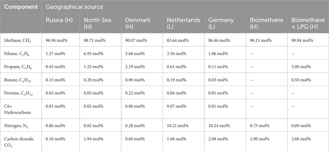
Table 1. Typical composition of natural gas proceeding from different geographical sources. Source: Deutscher Verein des Gas-und Wasserfaches, (2021).

One approach to characterising hydrogen-enriched natural gas would be the determination of the molar percentages of its most important components. A rigorous PGC-like, molecule-based approach would require the computation of nine unknowns, which can only be achieved if nine independent equations are available (one of them being given by the definition that the sum of the molar fractions is one). Recognising that the combination of pentane, hexane and higher hydrocarbons sums up less than about 0.1 mol%, their contribution can be either ignored or attributed to a slightly higher amount of butane without causing a significant error. Even so, 7 M percentages remain to be determined, which requires at least six independent physical measurements.

The difficulty in determining the full composition of this complex mixture has led some to search for correlation tendencies (Huber et al., 2018). What is of interest to the application is not the molar percentage of every component, but only that of hydrogen, alongside the overall combustion enthalpy. Hence, if an empirical combination of physical variables can be found, such that the two sought-after variables can be predicted within some accuracy, the computation of the composition can be avoided. Such a finding cannot be guaranteed, as it does not follow from a rigorous model, but it would be of great practical value if it is confirmed. In this article, we test some of the proposed correlation tendencies, finding negative results. The possibility of developing a machine-learning algorithm to predict these two variables based on a certain set of measurable properties, however numerous, remains an open possibility to be explored.

We address the question of a plausible physical characterisation with a different approach, considering hydrogen-enriched natural gas, not as a mixture of gas molecules, but as a mixture of mixtures. This is illustrated in Figure 1. Under this approach, each source of natural gas is characterised by a fixed composition and therefore by a set of effective thermodynamic properties that could serve as its fingerprint. If a certain user draws natural gas from two different sources and hydrogen is added to it, the quantification problem reduces to solving a system of two equations with two unknowns. This assumption is only valid for ideal gases, where molecule-molecule interactions are neglected. Therefore, our approach is limited to pressures less than about 10 bar (Cézar de Almeida et al., 2014) and so not applicable to ‘high-pressure’ pipelines, which are designed for pressures above 16 bar (Télessy et al., 2024). In the case of real-gas behaviour, further variables and more complex equations are required to characterise the mixture.

Figure 1

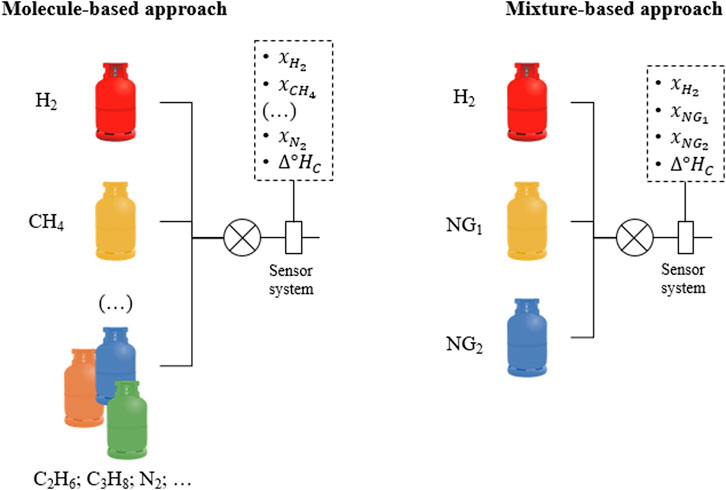
Figure 1. Illustration of two possible approaches to conceive the blending of hydrogen into natural gas, either as a combination of molecules or as a “mixture of mixtures” (valid only for ideal gases).

With a mixture-based approach, a system of equations of the following sort (Equation 1) is solved:

${\mathit{x}}_{\mathit{H}}+{\mathit{x}}_{\mathbf{1}}+\cdots +{\mathit{x}}_{\mathit{n}}=\mathbf{1}$

$\left\{\begin{array}{l}{\mathit{f}}_{\mathit{i}}\left({\mathit{x}}_{\mathit{H}},{\mathit{x}}_{\mathbf{1}},\dots ,{\mathit{x}}_{\mathit{n}}\right)={\mathit{y}}_{\mathit{i}}\\ \dots \end{array}\right.(1)$

where $x_H$ is the amount fraction of $H_2$, $x_{1\dots n}$ the amount fractions of the different ‘kinds’ of natural gas, and $y_i$ is a physical property that can be explicitly calculated as a function of the molar percentages. Solving for all the involved molar percentages, not just that of hydrogen, is important in order to estimate the enthalpy of combustion (Equation 2).

$\mathbf{\Delta }{\mathit{H}}_{\mathit{C}}={\mathit{x}}_{\mathit{H}}\mathbf{\Delta }{\mathit{H}}_{\mathit{H}}+{\displaystyle \sum _{\mathit{k}=\mathbf{1}}^{\mathit{n}}}{\mathit{x}}_{\mathit{k}}\mathbf{\Delta }{\mathit{H}}_{\mathit{k}}(2)$

If a sensor system is capable of estimating the enthalpy of combustion, the rate of energy transported through the gas can be then computed according to Equation 3, assuming ideal gas behaviour. (Let $v$ be the flow velocity, $A$ the area of the cross section of the conduit, $P$ the absolute pressure, $R$ the ideal gas constant, and $T$ the absolute temperature.) In other words, a sensor system for billing purposes requires a measurement of flow velocity, absolute pressure, and temperature.

$\dot{\mathit{E}}=\dot{\mathit{n}}\left|\mathbf{\Delta }\right.{\mathit{H}}_{\mathit{C}}\left|=\right.\left(\frac{\mathit{v}\mathit{A}\mathit{P}}{\mathit{R}\mathit{T}}\right)\left|\mathbf{\Delta }|{\mathit{H}}_{\mathit{C}}\right|(3)$

The ease or difficulty of solving this problem lies in the nature of the equations for each physical property, $y_i$. There ought to be an explicit equation under which each property can be directly related to each amount fraction. The equations need not be linear nor polynomial, but any valid approximation as either of these would significantly reduce the complexity.

2.2 Calculation of thermodynamic properties of a gas mixture

Let us now consider the available models through which the aforementioned thermodynamic properties (density, speed of sound, thermal conductivity and viscosity) can be calculated for a mixture of gases.

The ideal gas equation yields a simple linear model to calculate the density of a gas mixture (Equation 4) Rather than density itself ($\rho$), it is more convenient to refer to the molar mass ($M$) of the mixture, for it is independent on the absolute pressure and temperature. A measurement of density, therefore, ought to be accompanied by pressure and temperature sensors in order to make the respective compensation. This molar mass is simply the linear combination of the individual molar masses and the respective molar percentages. Notice that this linear combination can be expressed both in terms of the individual molecules and in terms of the different sources of natural gas.

$\frac{\mathit{\rho }\mathit{R}\mathit{T}}{\mathit{P}}=\mathit{M}=\sum {\mathit{M}}_{\mathit{i}}{\mathit{x}}_{\mathit{i}}(4)$

The Newton-Laplace equation for the speed of sound ($c$) in an ideal gas reveals its dependence on the overall molar mass of the mixture ($M$), as well as on the overall molar isobaric heat capacity ($C_p$) and molar isochoric heat capacity ($C_v$), all of which are given by linear combinations of the individual amount fractions (Dixon and Greenwood, 1925). Given the temperature dependence of the speed of sound, it is more convenient to calculate the ratio $RT/c^2$, which has units of molar mass and is denoted here as $M^{*}$ (Equation 5). The presence of linear combinations for the calculation of $C_p$, $C_v$ and $M$ also makes it possible to express the speed of sound in terms of either the molar percentages of the individual molecules or of the different ‘mixtures’ in the mixture (each with effective values of $C_p$, $C_v$ and $M$).

$\frac{\mathit{R}\mathit{T}}{{\mathit{c}}^{\mathbf{2}}}={\mathit{M}}^{*}=\frac{\left(\sum {\mathit{C}}_{\mathit{v}\mathit{i}}{\mathit{x}}_{\mathit{i}}\right)\left(\sum {\mathit{M}}_{\mathit{i}}{\mathit{x}}_{\mathit{i}}\right)}{\left(\sum {\mathit{C}}_{\mathit{p}\mathit{i}}{\mathit{x}}_{\mathit{i}}\right)}(5)$

Closer examination of Equation 5 leads to the observation that a quadratic polynomial of the individual amount fractions is always formed. For the case of hydrogen mixed with two different compositions of natural gas ($x_1$ and $x_2$, with $x_2=1-x_H-x_1$), Equation 5 can be rewritten as the quadratic polynomial in Equation 6, whereby each coefficient (${\zeta }_{ij}$) originates from a multiplication between a heat capacity and a molar mass.

${\mathit{\zeta }}_{\mathbf{20}}{\mathit{x}}_{\mathit{H}}^{\mathbf{2}}+{\mathit{\zeta }}_{\mathbf{11}}{\mathit{x}}_{\mathit{H}}{\mathit{x}}_{\mathbf{1}}+{\mathit{\zeta }}_{\mathbf{02}}{\mathit{x}}_{\mathbf{1}}^{\mathbf{2}}+{\mathit{\zeta }}_{\mathbf{10}}{\mathit{x}}_{\mathit{H}}+{\mathit{\zeta }}_{\mathbf{01}}{\mathit{x}}_{\mathbf{1}}+{\mathit{\zeta }}_{\mathbf{00}}=\mathbf{0}(6)$

The calculation of the thermal conductivity and viscosity of a gas mixture—even of ideal gases—is not a straightforward task. Mason and Saxena (1958) developed an approximate formula for the thermal conductivity based on a rigorous analysis of the kinetic theory of gases. A similar work was performed by Wilke (1950) for the calculation of viscosity. Both equations are very similar in form, showing how the pairwise interactions between components affect the overall behaviour of the mixture.

The thermal conductivity of a mixture (${\kappa }_{mix}$) is thus calculated according to³ Equation 7:

${\mathit{\kappa }}_{\mathit{m}\mathit{i}\mathit{x}}={\displaystyle \sum _{\mathit{i}=\mathbf{1}}^{\mathit{n}}}\frac{{\mathit{\kappa }}_{\mathit{i}}}{\mathbf{1}+\frac{\mathbf{1}}{{\mathit{x}}_{\mathit{i}}}{\displaystyle \sum _{\mathit{j}=\mathbf{1},\mathit{j}\ne \mathit{i}}^{\mathit{j}=\mathit{n}}}{\mathit{x}}_{\mathit{j}}{\mathit{G}}_{\mathit{i}\mathit{j}}}$

${\mathit{G}}_{\mathit{i}\mathit{j}}=\frac{\mathbf{1.065}}{\mathbf{2}\sqrt{\mathbf{2}}}\frac{{\left[\mathbf{1}+{\left(\frac{{\mathit{\mu }}_{\mathit{i}}}{{\mathit{\mu }}_{\mathit{j}}}\right)}^{\frac{\mathbf{1}}{\mathbf{2}}}{\left(\frac{{\mathit{M}}_{\mathit{j}}}{{\mathit{M}}_{\mathit{i}}}\right)}^{\frac{\mathbf{1}}{\mathbf{4}}}\right]}^{\mathbf{2}}}{{\left[\mathbf{1}+\left(\frac{{\mathit{M}}_{\mathit{i}}}{{\mathit{M}}_{\mathit{j}}}\right)\right]}^{\frac{\mathbf{1}}{\mathbf{2}}}}(7)$

And the viscosity of a mixture (${\mu }_{mix}$) is calculated according to Equation 8:

${\mathit{\mu }}_{\mathit{m}\mathit{i}\mathit{x}}={\displaystyle \sum _{\mathit{i}=\mathit{i}}^{\mathit{n}}}\frac{{\mathit{\mu }}_{\mathit{i}}}{\mathbf{1}+\frac{\mathbf{1}}{{\mathit{x}}_{\mathit{i}}}{\displaystyle \sum _{\mathit{j}=\mathbf{1},\mathit{j}\ne \mathit{i}}^{\mathit{j}=\mathit{n}}}{\mathit{x}}_{\mathit{j}}{\mathit{\varphi }}_{\mathit{i}\mathit{j}}}$

${\mathit{\varphi }}_{\mathit{i}\mathit{j}}=\frac{{\left[\mathbf{1}+{\left(\frac{{\mathit{\mu }}_{\mathit{i}}}{{\mathit{\mu }}_{\mathit{j}}}\right)}^{\frac{\mathbf{1}}{\mathbf{2}}}{\left(\frac{{\mathit{M}}_{\mathit{j}}}{{\mathit{M}}_{\mathit{i}}}\right)}^{\frac{\mathbf{1}}{\mathbf{4}}}\right]}^{\mathbf{2}}}{\left(\frac{\mathbf{4}}{\sqrt{\mathbf{2}}}\right){\left[\mathbf{1}+\left(\frac{{\mathit{M}}_{\mathit{i}}}{{\mathit{M}}_{\mathit{j}}}\right)\right]}^{\frac{\mathbf{1}}{\mathbf{2}}}}(8)$

Both models assume that the individual thermal conductivities and viscosities of the components are known, and that they are all referred to the same temperature. A model to describe the dependence of these properties on the state variables is further required to make the corresponding compensation. A first approximation for ideal gases can be drawn from kinetic theory, whereby the thermal conductivity varies with the square root of temperature and is independent of pressure (Mason, 2023), similarly to the speed of sound.

The reader may notice that the form of Equations 7, 8 gives little opportunity for a closed-form solution of a system of equations. Such a system can be solved numerically with the aid of search algorithms, but it could be impractical for an implementation in a portable electronic device. Here we apply and test a second-order Taylor approximation, knowing that the definition of the problem limits the concentration of hydrogen to relatively small values and that natural gas is mostly composed of methane. We test this polynomial approximation against rigorously calculated properties calculated according to Equations 7, 8. This second-order approximation has the simpler form in Equation 9 for the case of a mixture of hydrogen plus three different sorts of natural gas ($\left\{x_1,x_2,x_3\right\}$ with $x_3=1-x_H-x_1-x_2$).

${\mathit{\kappa }}_{\mathit{m}\mathit{i}\mathit{x}}\approx {\mathit{\kappa }}_{\mathbf{200}}{\mathit{x}}_{\mathit{H}}^{\mathbf{2}}+{\mathit{\kappa }}_{\mathbf{020}}{\mathit{x}}_{\mathbf{1}}^{\mathbf{2}}+{\mathit{\kappa }}_{\mathbf{002}}{\mathit{x}}_{\mathbf{2}}^{\mathbf{2}}+{\mathit{\kappa }}_{\mathbf{110}}{\mathit{x}}_{\mathit{H}}{\mathit{x}}_{\mathbf{1}}+{\mathit{\kappa }}_{\mathbf{101}}{\mathit{x}}_{\mathit{H}}{\mathit{x}}_{\mathbf{2}}+{\mathit{\kappa }}_{\mathbf{011}}{\mathit{x}}_{\mathbf{1}}{\mathit{x}}_{\mathbf{2}}+{\mathit{\kappa }}_{\mathbf{100}}{\mathit{x}}_{\mathit{H}}+{\mathit{\kappa }}_{\mathbf{010}}{\mathit{x}}_{\mathbf{1}}+{\mathit{\kappa }}_{\mathbf{001}}{\mathit{x}}_{\mathbf{2}}+{\mathit{\kappa }}_{\mathbf{000}}(9)$

2.3 Estimation of the hydrogen content and combustion enthalpy with physical measurements

2.3.1 Two-sensor case

For the simpler case of a mixture of three components (that is, hydrogen plus two sorts of natural gas), only two physical variables would be required to estimate the hydrogen concentration and the combustion enthalpy. Depending on the choice of sensors, either a system of one quadratic equation and a linear equation or a system of two quadratic equations would be obtained. The former case is directly solved by substitution, collapsing into a single quadratic equation. In fact, if the quadratic variable is the speed of sound, the reader can verify that the system collapses into a linear equation ($A_2=0$) (Equation 10).

$\left\{\begin{array}{l}{\mathit{\zeta }}_{\mathbf{20}}{\mathit{x}}_{\mathit{H}}^{\mathbf{2}}+{\mathit{\zeta }}_{\mathbf{11}}{\mathit{x}}_{\mathit{H}}{\mathit{x}}_{\mathbf{1}}+{\mathit{\zeta }}_{\mathbf{02}}{\mathit{x}}_{\mathbf{1}}^{\mathbf{2}}+{\mathit{\zeta }}_{\mathbf{10}}{\mathit{x}}_{\mathit{H}}+{\mathit{\zeta }}_{\mathbf{01}}{\mathit{x}}_{\mathbf{1}}+{\mathit{\zeta }}_{\mathbf{00}}=\mathbf{0}\\ \left({\mathit{M}}_{\mathit{H}}-{\mathit{M}}_{\mathbf{2}}\right){\mathit{x}}_{\mathit{H}}+\left({\mathit{M}}_{\mathbf{1}}-{\mathit{M}}_{\mathbf{2}}\right){\mathit{x}}_{\mathbf{1}}=\left(\mathit{M}-{\mathit{M}}_{\mathbf{2}}\right)\end{array}\right.$

${\mathit{A}}_{\mathbf{2}}{\mathit{x}}_{\mathit{H}}^{\mathbf{2}}+{\mathit{A}}_{\mathbf{1}}{\mathit{x}}_{\mathit{H}}+{\mathit{A}}_{\mathbf{0}}=\mathbf{0}(10)$

Notice that the properties of the three components are subtracted from one another, evidencing how this method would fail to discriminate them if their properties are identical.

If the chosen variables are the speed of sound and the thermal conductivity, the amount fractions can be obtained with the fixed-point iteration method (Equation 11), starting with the guess ${\left[\begin{array}{cc}{x}_H& x_1\end{array}\right]}_0^T=\overrightarrow{0}$:

$\left\{\begin{array}{l}{\mathit{\zeta }}_{\mathbf{20}}{\mathit{x}}_{\mathit{H}}^{\mathbf{2}}+{\mathit{\zeta }}_{\mathbf{11}}{\mathit{x}}_{\mathit{H}}{\mathit{x}}_{\mathbf{1}}+{\mathit{\zeta }}_{\mathbf{02}}{\mathit{x}}_{\mathbf{1}}^{\mathbf{2}}+{\mathit{\zeta }}_{\mathbf{10}}{\mathit{x}}_{\mathit{H}}+{\mathit{\zeta }}_{\mathbf{01}}{\mathit{x}}_{\mathbf{1}}+{\mathit{\zeta }}_{\mathbf{00}}=\mathbf{0}\\ {\mathit{\kappa }}_{\mathbf{20}}{\mathit{x}}_{\mathit{H}}^{\mathbf{2}}+{\mathit{\kappa }}_{\mathbf{11}}{\mathit{x}}_{\mathit{H}}{\mathit{x}}_{\mathbf{1}}+{\mathit{\kappa }}_{\mathbf{02}}{\mathit{x}}_{\mathbf{1}}^{\mathbf{2}}+{\mathit{\kappa }}_{\mathbf{10}}{\mathit{x}}_{\mathit{H}}+{\mathit{\kappa }}_{\mathbf{01}}{\mathit{x}}_{\mathbf{1}}+{\mathit{\kappa }}_{\mathbf{00}}-\mathit{\kappa }=\mathbf{0}\end{array}\right.$

$\left[\begin{array}{cc}{\mathit{\zeta }}_{\mathbf{10}}& {\mathit{\zeta }}_{\mathbf{01}}\\ {\mathit{\kappa }}_{\mathbf{10}}& {\mathit{\kappa }}_{\mathbf{01}}\end{array}\right]{\left[\begin{array}{c}{\mathit{x}}_{\mathit{H}}\\ {\mathit{x}}_{\mathbf{1}}\end{array}\right]}_{\mathit{i}+\mathbf{1}}=\left[\begin{array}{c}-{\mathit{\zeta }}_{\mathbf{00}}\\ \mathit{\kappa }-{\mathit{\kappa }}_{\mathbf{00}}\end{array}\right]-\left[\begin{array}{cc}{\mathit{\zeta }}_{\mathbf{20}}{\mathit{x}}_{\mathit{H}}+\frac{\mathbf{1}}{\mathbf{2}}{\mathit{\zeta }}_{\mathbf{11}}{\mathit{x}}_{\mathbf{1}}& {\mathit{\zeta }}_{\mathbf{02}}{\mathit{x}}_{\mathbf{1}}+\frac{\mathbf{1}}{\mathbf{2}}{\mathit{\zeta }}_{\mathbf{11}}{\mathit{x}}_{\mathit{H}}\\ {\mathit{\kappa }}_{\mathbf{20}}{\mathit{x}}_{\mathit{H}}+\frac{\mathbf{1}}{\mathbf{2}}{\mathit{\kappa }}_{\mathbf{11}}{\mathit{x}}_{\mathbf{1}}& {\mathit{\kappa }}_{\mathbf{02}}{\mathit{x}}_{\mathbf{1}}+\frac{\mathbf{1}}{\mathbf{2}}{\mathit{\kappa }}_{\mathbf{11}}{\mathit{x}}_{\mathit{H}}\end{array}\right]{\left[\begin{array}{c}{\mathit{x}}_{\mathit{H}}\\ {\mathit{x}}_{\mathbf{1}}\end{array}\right]}_{\mathit{i}}(11)$

2.3.2 Three-sensor case

The more complex case of a mixture of four components (hydrogen plus three different sorts of natural gas) requires the measurement of three variables, such as density, speed of sound and thermal conductivity. The fortunate fact that substitution of the molar mass equation into the equation of the speed of sound results in a linear equation enables a solution of this system of three equations by direct substitution as well (Equation 12).

$\left\{\begin{array}{l}\left({\mathit{M}}_{\mathbf{1}}-{\mathit{M}}_{\mathbf{3}}\right){\mathit{x}}_{\mathbf{1}}+\left({\mathit{M}}_{\mathit{H}}-{\mathit{M}}_{\mathbf{3}}\right){\mathit{x}}_{\mathit{H}}+\left({\mathit{M}}_{\mathbf{2}}-{\mathit{M}}_{\mathbf{3}}\right){\mathit{x}}_{\mathbf{2}}=\left(\mathit{M}-{\mathit{M}}_{\mathbf{3}}\right)\\ {\mathit{\zeta }}_{\mathbf{200}}{\mathit{x}}_{\mathit{H}}^{\mathbf{2}}+{\mathit{\zeta }}_{\mathbf{020}}{\mathit{x}}_{\mathbf{1}}^{\mathbf{2}}+{\mathit{\zeta }}_{\mathbf{002}}{\mathit{x}}_{\mathbf{2}}^{\mathbf{2}}+{\mathit{\zeta }}_{\mathbf{110}}{\mathit{x}}_{\mathit{H}}{\mathit{x}}_{\mathbf{1}}+{\mathit{\zeta }}_{\mathbf{101}}{\mathit{x}}_{\mathit{H}}{\mathit{x}}_{\mathbf{2}}+{\mathit{\zeta }}_{\mathbf{011}}{\mathit{x}}_{\mathbf{1}}{\mathit{x}}_{\mathbf{2}}\\ +{\mathit{\zeta }}_{\mathbf{100}}{\mathit{x}}_{\mathit{H}}+{\mathit{\zeta }}_{\mathbf{010}}{\mathit{x}}_{\mathbf{1}}+{\mathit{\zeta }}_{\mathbf{001}}{\mathit{x}}_{\mathbf{2}}+{\mathit{\zeta }}_{\mathbf{000}}=\mathbf{0}\\ {\mathit{\kappa }}_{\mathbf{200}}{\mathit{x}}_{\mathit{H}}^{\mathbf{2}}+{\mathit{\kappa }}_{\mathbf{020}}{\mathit{x}}_{\mathbf{1}}^{\mathbf{2}}+{\mathit{\kappa }}_{\mathbf{002}}{\mathit{x}}_{\mathbf{2}}^{\mathbf{2}}+{\mathit{\kappa }}_{\mathbf{110}}{\mathit{x}}_{\mathit{H}}{\mathit{x}}_{\mathbf{1}}+{\mathit{\kappa }}_{\mathbf{101}}{\mathit{x}}_{\mathit{H}}{\mathit{x}}_{\mathbf{2}}+{\mathit{\kappa }}_{\mathbf{011}}{\mathit{x}}_{\mathbf{1}}{\mathit{x}}_{\mathbf{2}}\\ +{\mathit{\kappa }}_{\mathbf{100}}{\mathit{x}}_{\mathit{H}}+{\mathit{\kappa }}_{\mathbf{010}}{\mathit{x}}_{\mathbf{1}}+{\mathit{\kappa }}_{\mathbf{001}}{\mathit{x}}_{\mathbf{2}}+{\mathit{\kappa }}_{\mathbf{000}}=\mathit{\kappa }\end{array}\right)(12)$

Substitution of the first equation into both the second and third one leads to a system of the following sort (Equation 13):

$\left\{\begin{array}{l}{\mathit{C}}_{\mathbf{20}}{\mathit{x}}_{\mathit{H}}^{\mathbf{2}}+{\mathit{C}}_{\mathbf{02}}{\mathit{x}}_{\mathbf{1}}^{\mathbf{2}}+{\mathit{C}}_{\mathbf{11}}{\mathit{x}}_{\mathit{H}}{\mathit{x}}_{\mathbf{1}}+{\mathit{C}}_{\mathbf{10}}{\mathit{x}}_{\mathit{H}}+{\mathit{C}}_{\mathbf{01}}{\mathit{x}}_{\mathbf{1}}+{\mathit{C}}_{\mathbf{00}}=\mathbf{0}\\ {\mathit{K}}_{\mathbf{20}}{\mathit{x}}_{\mathit{H}}^{\mathbf{2}}+{\mathit{K}}_{\mathbf{02}}{\mathit{x}}_{\mathbf{1}}^{\mathbf{2}}+{\mathit{K}}_{\mathbf{11}}{\mathit{x}}_{\mathit{H}}{\mathit{x}}_{\mathbf{1}}+{\mathit{K}}_{\mathbf{10}}{\mathit{x}}_{\mathit{H}}+{\mathit{K}}_{\mathbf{01}}{\mathit{x}}_{\mathbf{1}}+\left({\mathit{K}}_{\mathbf{00}}-\mathit{\kappa }\right)=\mathbf{0}\end{array}\right.(13)$

The reader is encouraged to verify that the second-order coefficients of the first equation—$C_{20}$, $C_{02}$ and $C_{11}$—are all zero. Hence, the amount fraction of hydrogen can be solved with a simple quadratic equation (Equation 14):

${\mathit{P}}_{\mathbf{2}}{\mathit{x}}_{\mathit{H}}^{\mathbf{2}}+{\mathit{P}}_{\mathbf{1}}{\mathit{x}}_{\mathit{H}}+{\mathit{P}}_{\mathbf{0}}=\mathbf{0}(14)$

2.4 Monte-Carlo simulation

In order to verify the accuracy of the proposed estimation methods, a set of randomly generated—yet feasible—natural gas compositions were calculated. Table 2 shows the tabulated properties of the relevant molecules at 20°C and atmospheric pressure, extracted from the NIST database (Lemmon et al., 2023). With this information, the thermodynamic properties of several random mixtures of natural gas and hydrogen can be computed, using the models in Equations 3, 4, 6, 7. We ‘synthesised’ thus one hundred random binary combinations of the seven natural gas sources in Table 1 and then calculated their properties upon mixture with hydrogen from 0 mol% to 30 mol%. If the proposed estimators are able to compute the combustion enthalpy and the hydrogen content of such a wide spectrum of natural gas compositions, such a system can certainly be calibrated for a more regulated application case.

Table 2

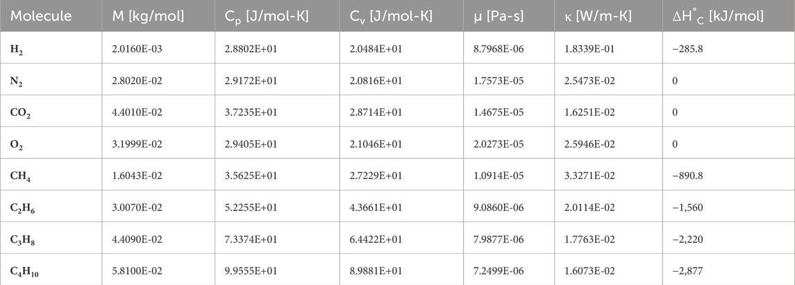
Table 2. Thermodynamic properties of gas molecules contained in hydrogen-enriched natural gas. Source: Lemmon et al. (2023). All properties are tabulated for 20°C and atmospheric pressure, except for the standard combustion enthalpy, which corresponds to 25°C and 100 kPa.

In this study, we compare four kinds of estimators with increasing complexity. The simplest estimator is based on a measurement of the thermal conductivity alone and is calibrated against one source of natural gas (“NG type 1” in Figure 2). It naïvely assumes that there is no variation in the composition of natural gas, and any change in the thermal conductivity is attributed to a change in the hydrogen content alone. The combustion enthalpy is then simply calculated as the linear combination of the enthalpy of hydrogen and that of the calibration gas with the corresponding proportions. The following two estimators are based on two variables⁴—speed of sound together with thermal conductivity, and density together with thermal conductivity. A two-variable estimator requires a calibration with two sources of natural gas, and it assumes that any variation in the composition of natural gas is due to a combination of these two sources. It is therefore convenient to select an “H” gas and an “L” gas for this purpose. If only these two sources (and hydrogen) are randomly blended, this method would exhibit virtually no detection error. The final estimator whose performance will be evaluated is based on the combined measurement of the three mentioned variables (thermal conductivity, speed of sound and density). This estimator was calibrated with the three types of natural gas whose thermal conductivity is shown in Figure 2 (an “H” gas, an “L” gas, and a type of biomethane). Its underlying assumption is that any variation in the constitution of natural gas is due to a ternary mixture of these three sorts. This estimator is therefore expected to be much more robust against composition variations, detecting both the concentration of hydrogen and the combustion enthalpy with a high precision—in spite of there being seven different sources of natural gas, mixed binarily in random proportions. The accuracy of these four estimation methods was evaluated with the root-mean-square error (Equation 15) in the prediction of the variables of interest (combustion enthalpy and molar fraction of hydrogen) for all the randomly generated mixtures.

${\mathit{ϵ}}_{\mathit{R}\mathit{M}\mathit{S}}=\sqrt{\frac{\mathbf{1}}{\mathit{N}}\sum {\left(\frac{{\mathit{x}}_{\mathit{p}\mathit{r}\mathit{e}\mathit{d}\mathit{i}\mathit{c}\mathit{t}}-{\mathit{x}}_{\mathit{t}\mathit{r}\mathit{u}\mathit{e}}}{{\mathit{x}}_{\mathit{t}\mathit{r}\mathit{u}\mathit{e}}}\right)}^{\mathbf{2}}}(15)$

Figure 2

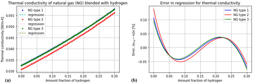
Figure 2. Test of the proposed quadratic model of Equation 8 to predict the thermal conductivity of a mixture of three different sources of natural gas with hydrogen. Types “1”, “2” and “3” correspond to the sources “Russia”, “Netherlands” and “Biomethane” in Table 1, respectively. (A) Variation of the thermal conductivity with the amount fraction of hydrogen. (B) Error of the quadratic model.

The previous comparison assumes that the measurement of the physical variables is free from experimental error, which is unrealistic. For this reason, a second study was performed, in which the outcome of each physical measurement is distorted by a Gaussian distribution with varying degrees of standard deviation (0.5%, 1.0% and 2.0% of the mean). Therefore, for every randomly generated gas mixture, a series of 30 “measurements” of the physical variables under the influence of said cases of experimental error were performed, in order to assess the robustness of the proposed detection methods in a realistic scenario. It is expected that the three-variable estimator will suffer a higher loss of accuracy under the effect of experimental uncertainty than the two- or one-variable ones.

3 Results

3.1 Regression model for the thermal conductivity

We proposed in Section 2.2 to simplify the calculation of the thermal conductivity of a mixture (Equation 7) as a quadratic polynomial (Equation 9). It can be seen in Figure 2 that the coefficients of such a polynomial can be fitted with a least-squares procedure to predict the thermal conductivity with high precision. These coefficients were fitted using the simulated curves of thermal conductivity vs amount fraction of hydrogen for three selected sources of natural gas (one ‘H’-type, one ‘L’-type and a type of biomethane). Such a polynomial fit could be obtained with experimental data by measuring the thermal conductivity of each independent natural gas source upon hydrogen addition in the concentration range of interest. This quadratic model facilitates the solution of a system of equations to a great extent. Some have proposed to use a linear fit for the thermal conductivity (Huber et al., 2018), but this would result in a loss of precision.

In order to find an appropriate fit of the constants in Equation 9, we suggest using an optimisation routine with a first guess based on the separate regressions of the conductivity-concentration curves of the three independent natural gas sources used for calibration. The substitution for each separate combination of natural gas and hydrogen leads in each case to a simplification of the complete polynomial, as shown in Equation 16. The first case corresponds to $\left\{x_2=0;x_1=1-x_H\right\}$; the second case corresponds to $\left\{x_1=0;x_2=1-x_H\right\}$; and the third case to $\left\{x_1=0;x_2\left.=0\right\}\right.$. From each case, a set of three constants can be directly obtained by a standard polynomial regression; however, the nine constants that are obtained cannot be used directly to calculate the ten constants required by Equation 9. Our suggestion is to set all cross-coefficients $\left\{{\kappa }_{110},{\kappa }_{101},{\kappa }_{011}\right\}$ to zero, which enables obtaining the initial guess of the rest of the constants by direct substitution. The actual coefficients can be then obtained by a minimisation of the sum of the root-mean square error of all three curves against the complete polynomial.

$\left\{\begin{array}{l}\left({\kappa }_{200}+{\kappa }_{020}-{\kappa }_{110}\right)x_H^2+\left({\kappa }_{100}-2{\kappa }_{020}+{\kappa }_{110}-{\kappa }_{010}\right)x_H+\left({\kappa }_{020}+{\kappa }_{010}+{\kappa }_{000}\right)=\kappa \\ \left({\kappa }_{200}+{\kappa }_{002}-{\kappa }_{101}\right)x_H^2+\left({\kappa }_{100}-2{\kappa }_{002}+{\kappa }_{101}-{\kappa }_{001}\right)x_H+\left({\kappa }_{002}+{\kappa }_{001}+{\kappa }_{000}\right)=\kappa \\ {\kappa }_{200}{x}_H^2+{\kappa }_{100}{x}_H+{\kappa }_{000}=\kappa \end{array}\right)(16)$

3.2 Variation of the thermodynamic properties of natural gas

The variation in the speed of sound, density, thermal conductivity and viscosity of all the randomly generated natural gas compositions can be observed in Figure 3. One can appreciate how the variation in the composition of natural gas has a non-negligible impact in the speed of sound and density, a mild effect in the thermal conductivity, and a dominant role in the viscosity. It is noticeable that, for instance, a reading of 460 m/s in the speed of sound corresponds to 10 mol% $H_2$ in one end and to 20 mol% $H_2$ in the opposite end of the spectrum of natural gas composition. If such a variation in the constitution of natural gas is present in a real application, the measurement of just the speed of sound or density would be inadequate to predict the amount fraction of hydrogen. On the other hand, the high sensitivity of the thermal conductivity to the presence of hydrogen, combined with a relative insensitivity to the variation in the composition of natural gas, makes this variable very appealing for estimating the hydrogen content. The opposite case is observed in the viscosity, whose variation with the amount fraction of hydrogen (at least in the range until 30 mol%) is rather negligible, whereas its sensitivity to the composition of natural gas is very high.

Figure 3

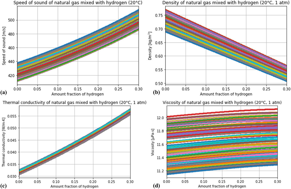
Figure 3. Calculation of four thermodynamic properties—(A) speed of sound, (B) density, (C) thermal conductivity and (D) viscosity—for several random compositions of natural gas blended with hydrogen.

3.3 Performance of the proposed estimators

Having calculated the thermodynamic properties of several random gas mixtures, the accuracy of the methods proposed in Section 2.3. Can be evaluated. In spite of ignoring the variations in the composition of natural gas, the one-variable estimator based on the thermal conductivity predicts the hydrogen content relatively well, with an expected deviation around ±2 mol%. Such a deviation would be inadequate for low $H_2$ concentrations (e.g., 5 mol%) but uncritical for higher concentrations (e.g., 30 mol%). Figure 4 shows the root mean square error of the estimator as a function of the hydrogen concentration. The expected error in the estimation of the combustion enthalpy is close to 5%, which could be tolerable for household billing applications. By measuring an additional variable to the thermal conductivity (whether density or the speed of sound), the two-variable estimator was able to reduce the error in the prediction of the amount fraction of hydrogen significantly. Nevertheless, there seems to be no improvement in the estimation of the combustion enthalpy. The three-variable estimator, whilst retaining a comparable error in the prediction of the amount fraction of hydrogen in comparison to the two-variable cases, was able to further improve the accuracy of the prediction of the combustion enthalpy.

Figure 4

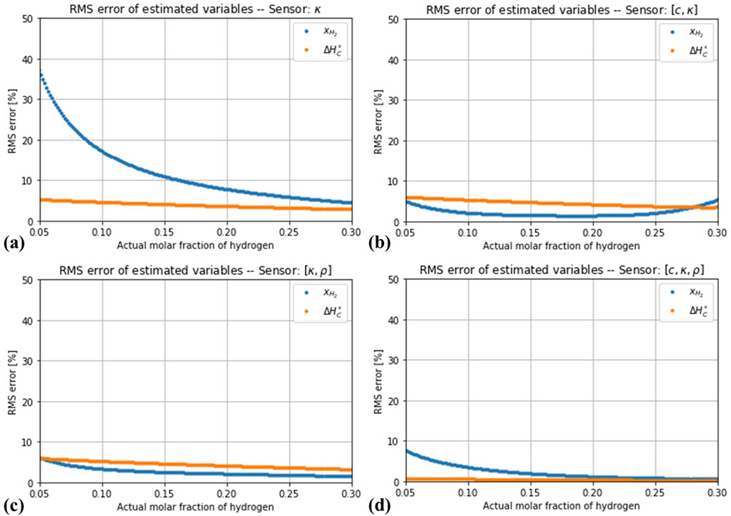
Figure 4. Root-mean square error in the estimation of the hydrogen concentration and the enthalpy of combustion of several random blends of natural gas and hydrogen. (A) Estimation using thermal conductivity alone. (B) Estimation with thermal conductivity and speed of sound. (C) Estimation with thermal conductivity and density. (D) Estimation with all three variables.

If the effect of a random measurement uncertainty is considered, the simultaneous measurement of more variables does not automatically lead to a more robust estimation. As Figure 5 shows, the impact of the simulated noise levels is negligible for the estimator based on only one variable (thermal conductivity). A different situation is observed for the estimators based on two variables, as shown in Figures 6, 7. The estimation of the hydrogen content was increasingly distorted with the introduced noise, whereas the estimation of the combustion enthalpy remained unaffected. With a measurement error of 2% in both variables, the estimator based on speed of sound and thermal conductivity performed no better than the one based on thermal conductivity alone, and the one based on thermal conductivity and density performed only slightly better. The final case of a three-variable estimator showed, as expected, a very high sensitivity to the introduced noise (Figures 8). Only if the noise in all three variables is kept below 1% does it show an advantage compared to the one-variable estimator.

Figure 5

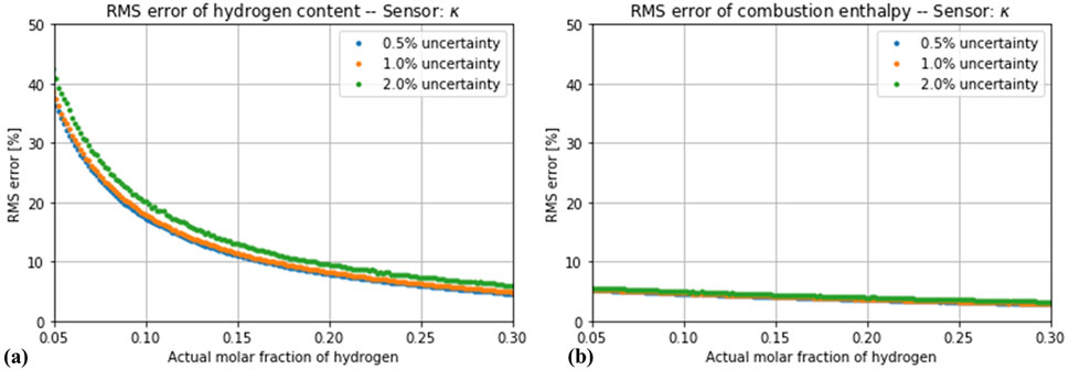
Figure 5. Root-mean square error in the estimation of (A) hydrogen concentration and (B) enthalpy of combustion by the estimator based on thermal conductivity alone, assuming a total measurement error of 0.5%, 1% and 2%.

Figure 6

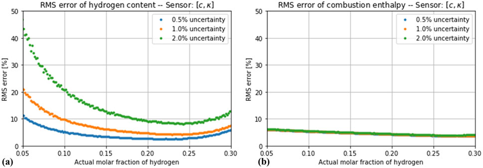
Figure 6. Root-mean square error in the estimation of (A) hydrogen concentration and (B) enthalpy of combustion by the estimator based on thermal conductivity and speed of sound, assuming a total measurement error of 0.5%, 1% and 2%.

Figure 7

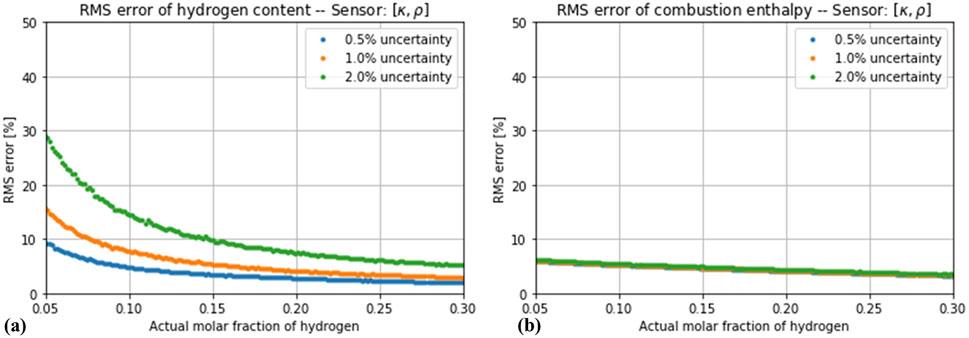
Figure 7. Root-mean square error in the estimation of (A) hydrogen concentration and (B) enthalpy of combustion by the estimator based on thermal conductivity and density, assuming a total measurement error of 0.5%, 1% and 2%.

Figure 8

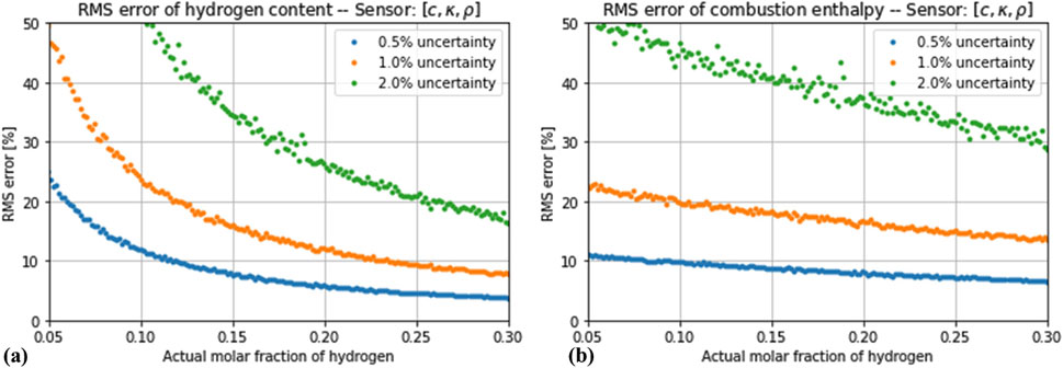
Figure 8. Root-mean square error in the estimation of (A) hydrogen concentration and (B) enthalpy of combustion by the estimator based on thermal conductivity, speed of sound and density, assuming a total measurement error of 0.5%, 1% and 2%.

Considering all these effects, the combination of thermal conductivity and either density or speed of sound seem to offer a good trade-off between robustness against random variations and robustness against noise. These two estimators outperform the measurement of thermal conductivity alone, as long as the total measurement uncertainty of both variables is kept around or below 1%. Although the measurement of thermal conductivity and density seems to be less sensitive to measurement noise with respect to the case with the speed of sound, the measurement of density is affected by the propagated error proceeding from the temperature and pressure compensation that it requires (whereas the speed of sound only requires a temperature compensation). A further advantage of measuring the speed of sound is that, if it is determined by an ultrasonic system, such a device will naturally also provide the measurement of the flow velocity, which is necessary for computing the energy consumption (Equation 3).

3.4 Performance of correlation methods

It has been suggested that the heating value of natural gas (without blending hydrogen into it) can be correlated to some thermodynamic properties (Huber et al., 2018). In particular, the higher heating value ($HHV=-\frac{\rho }{M}\Delta °H_c$) is said to correlate with density, whereas the Wobbe index ($Wo=HHV/\sqrt{\rho /{\rho }_{air}}$) with viscosity. With the randomly calculated mixtures in our Monte-Carlo simulation, we do not observe a clear tendency between these variables, as Figure 9 shows. However, we cannot discard the possibility of a correlation based on a more sophisticated combination of these variables and perhaps some additional ones.

Figure 9

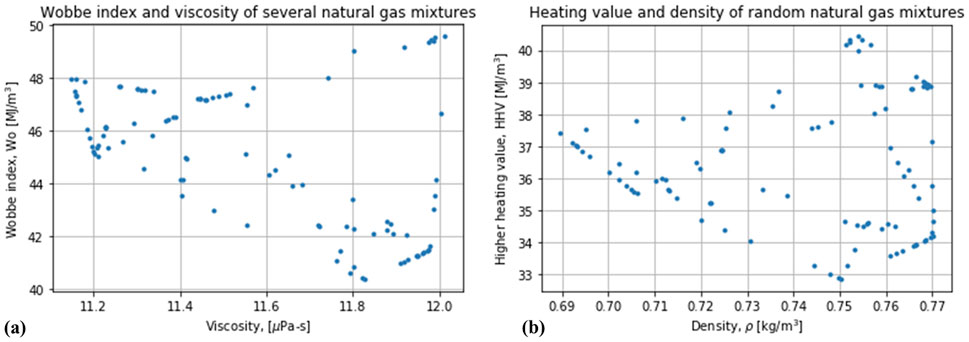
Figure 9. Evaluation of possible correlations of the heating value of random mixtures of natural gas (not blended with hydrogen) against some thermodynamic variables: (A) Wobbe index vs viscosity, (B) Higher heating value vs. density.

4 Conclusion

A combination of physical sensors can be used to monitor blends of natural gas and hydrogen, estimating both the amount fraction of hydrogen and the combustion enthalpy of the mixture. A methodology for this purpose was laid out in this work, based on the assumption of ideal-gas behaviour, which allows conceiving natural gas as a “mixture of mixtures” instead of a “mixture of molecules”. Under this paradigm, variations in the composition of natural gas can be understood as the mixture of different ‘types’ of natural gas with a fixed composition, and a system of up to three equations and three unknowns can be formulated in order to determine the amount fraction of each “type” of natural gas that is believed to compose the total blend. Therefore, the combustion enthalpy of the blend and its amount fraction of hydrogen can be estimated by measuring up to three physical variables simultaneously (thermal conductivity, speed of sound, and density), with varying degrees of robustness against variations in the source of natural gas and sensitivity to the uncertainty of the measurements. Our Monte-Carlo simulation reveals that an estimator based on the measurement of thermal conductivity together with either speed of sound or density is capable of correcting the deviations caused by the variability of natural gas, as long as the total measurement error is kept within 1% in both variables. For applications where the previous assumptions are not met, a more robust, real-time monitoring technique can be developed by combining the measurement of these thermodynamic properties with infrared spectroscopy.

Data availability statement

The raw data supporting the conclusions of this article will be made available by the authors, without undue reservation.

Author contributions

JM: Conceptualization, Formal Analysis, Investigation, Methodology, Software, Validation, Writing–original draft, Writing–review and editing.

Funding

The author(s) declare that financial support was received for the research, authorship, and/or publication of this article. This work was supported by the Fraunhofer Internal Programmes under Grant No. SME 685 400.

Conflict of interest

The author declares that the research was conducted in the absence of any commercial or financial relationships that could be construed as a potential conflict of interest.

Publisher’s note

All claims expressed in this article are solely those of the authors and do not necessarily represent those of their affiliated organizations, or those of the publisher, the editors and the reviewers. Any product that may be evaluated in this article, or claim that may be made by its manufacturer, is not guaranteed or endorsed by the publisher.

Footnotes

¹For a review on the development of this technique, see Bartle and Myers, 2002.

²Micro Electro Mechanical Systems

³The ratio of the individual viscosities instead of individual thermal conductivities in the calculation of $G_{ij}$ is not an error but a result of kinetic theory.

⁴The combination of density and speed of sound is also a possibility; however, the response of an estimator based on the density and speed of sound is not robust enough against the inclusion of a third source of natural gas.

References

Ajanovic, A., and Haas, R. (2018). On the long-term prospects of power-to-gas technologies. Wiley Interdiscip. Rev. Energy Environ. 8, 1. doi:10.1002/wene.318

CrossRef Full Text | Google Scholar

Bartle, K. D., and Myers, P. (2002). History of gas chromatography. TrAC. 21 (9+10), 547–557. doi:10.1016/S0165-9936(02)00806-3

CrossRef Full Text | Google Scholar

Benkendorf, M. (2023). Compact thermal conductivity detector. Whitepaper. Available online at: https://www.ipm.fraunhofer.de/content/dam/ipm/en/PDFs/product-information/GP/TMS/Thermal-conductivity-sensor-hydrogen.pdf.

Google Scholar

Bolwien, C. (2022). Quantifying gas mixtures - hydrogen and gaseous fuels. Whitepaper. Available online at: https://www.ipm.fraunhofer.de/content/dam/ipm/en/PDFs/product-information/GP/SPA/Quantifying-gas-mixtures-IR-spectroscopy.pdf.

Google Scholar

Cerbe, G., and Lendt, B. (2017). Grundlagen der Gastechnik. Munich: Carl Hanser Verlag.

Google Scholar

Cézar de Almeida, J., Velásquez, J. A., and Barbieri, R. (2014). A methodology for calculating the natural gas compressibility factor for a distribution network. Pet. Sci. Technol. 32, 2616–2624. doi:10.1080/10916466.2012.755194

CrossRef Full Text | Google Scholar

Deutscher Verein des Gas- und Wasserfaches (2021). Tech. Regel – Arbeitsblatt DVGW G. 260 (A) Gasbeschaffenheit.

Google Scholar

Dixon, H. B., and Greenwood, G. (1925). On the velocity of sound in mixtures of gases. Proc. R. Soc. A Math. Phys. Eng. Sci. 109 (752), 561–569.

Google Scholar

Dörr, H., Kröger, K., Graf, F., Köppel, W., Burmeister, F., Senner, J., et al. (2016). Untersuchungen zur Einspeisung von Wasserstoff in ein Erdgasnetz. DVGW Energ. | Wasser Prax. 11, 50–59. doi:10.1098/rspa.1925.0145

CrossRef Full Text | Google Scholar

Fodor, G. E. (1996). Analysis of natural gas by Fourier transform infrared spectroscopy. U. S. Army TARDEC Fuels Lubr. Res. Facil. (SwRI). TFLRF No. 319.

Google Scholar

Franco, A., and Rocca, M. (2024). Industrial decarbonization through blended combustion of natural gas and hydrogen. Hydrogen 5, 519–539. doi:10.3390/hydrogen5030029

CrossRef Full Text | Google Scholar

Huber, C., Reith, P., and Badarlis, A. (2018). Verfahren zum Bestimmen von Eigenschaften eines kohlenwasserstoffhaltigen Gasgemisches und Vorrichtung dafür. Published German patent application DE 10 2016 121 226 A1

Google Scholar

Lemmon, E. W., Bell, I. H., Huber, M. L., and McLinden, M. O. (2023). “Thermophysical properties of fluid systems,” in NIST chemistry WebBook, NIST standard reference database number 69. Editors P. J. Linstrom, and W. G. Mallard (Gaithersburg MD, 20899: National Institute of Standards and Technology). doi:10.18434/T4D303

CrossRef Full Text | Google Scholar

Liu, W., Wen, F., and Xue, Y. (2017). Power-to-gas technology in energy systems: current status and prospects of potential operation strategies. J. Mod. Power Syst. Clean. Energy. 5, 439–450. doi:10.1007/s40565-017-0285-0

CrossRef Full Text | Google Scholar

Makaryan, I. A., Sedov, I. V., Salgansky, E. A., Arutyunov, A. V., and Arutyunov, V. A. (2022). A comprehensive review on the prospects of using hydrogen-methane blends: challenges and opportunities. Energies 15, 2265. doi:10.3390/en15062265

CrossRef Full Text | Google Scholar

Mason, E. A. (2023). “Gas,” in Encyclopedia britannica. Available online at: https://www.britannica.com/science/gas-state-of-matter.

Google Scholar

Mason, E. A., and Saxena, S. C. (1958). Approximate formula for the thermal conductivity of gas mixtures. Phys. Fluids. 1 (5), 361–369. doi:10.1063/1.1724352

CrossRef Full Text | Google Scholar

Melaina, M. W., Antonia, O., and Penev, M. (2013). Blending hydrogen into natural gas pipeline networks: a review of key issues. National Renewable Energy Laboratory. NREL/TP-5600-51995.

Google Scholar

Monsalve, J. M., Völz, U., Jongmanns, M., Betz, B., Langa, S., Ruffert, C., et al. (2022). Rapid characterisation of mixtures of hydrogen and natural gas by means of ultrasonic time-delay estimation. J. Sens. Sens. Syst. 13, 179–185. doi:10.5194/jsss-13-179-2024

CrossRef Full Text | Google Scholar

Müller-Syring, G., and Henel, M. (2014). Wasserstofftoleranz der Erdgasinfrastruktur inklusive aller assoziierten Anlagen. Dtsch. Ver. Gas- Wasserfaches e.V. Abschlussbericht 1-02-12. Available online at: https://www.dvgw.de/medien/dvgw/forschung/berichte/g1_02_12.pdf.

Google Scholar

Télessy, K., Barner, L., and Holz, F. (2024). Repurposing natural gas pipelines for hydrogen: limits and options from a case study in Germany. Int. J. Hydrog. Energy. 80, 821–831. doi:10.1016/j.ijhydene.2024.07.110

CrossRef Full Text | Google Scholar

Wilke, C. R. (1950). A viscosity equation for gas mixtures. J. Chem. Phys. 18 (4), 517–519. doi:10.1063/1.1747673

CrossRef Full Text | Google Scholar