Augmented pre-training-based carbon emission accounting method using electricity data under small-sample condition

Introduction: Accurate and rapid carbon accounting method for the power industry is crucial to support China’s low-carbon transformation. Currently, carbon emission accounting methods are based on slowly updated fuel statistics or expensive monitoring equipment, resulting in high costs and delays in carbon emission estimation. Power data offers high real-time availability, accuracy, and resolution, and exhibits a strong correlation with carbon emissions. These characteristics provide a pathway for achieving rapid and precise annual carbon emission accountings. However, carbon emission data inherently exhibits small sample characteristics, making these methods less effective in small sample conditions and leading to lower accounting accuracy.

Methods: Therefore, this paper proposes an augmented pre-training-based “electricity-to-carbon” method under small sample conditions.

Results: This approach utilizes the correlation between electricity and carbon data as well as the autocorrelation characteristics of carbon emission data to construct a machine learning-based electricity-carbon fitting model for rapid and accurate carbon emission estimation. To address the challenges of small sample learning, this paper introduces an interpolation pre-training method to optimize the model’s hyperparameters and conserve samples for model training, thereby improving the model’s generalization and robustness.

Discussion: Case studies on a real dataset verifies the effectiveness of the proposed method. The findings of this study can promote the development of carbon measurement technology and facilitate the low-carbon transition of developing countries.

1 Introduction

Since the Industrial Revolution, global greenhouse gas emissions have continuously increased, leading to increasingly severe climate issues (IEA, 2023). Controlling greenhouse gas emissions and addressing climate change have become critical challenges that countries must face. In 2020, China proposed the “carbon peak and carbon neutrality” goal, regarded as powerful measures to tackle global climate issues (Jiang et al., 2022).

Accurate and rapid carbon emission accounting methods are fundamental for various entities to undertake low-carbon initiatives, playing a vital guiding and supportive role (Wang et al., 2024). Currently, methods for annual carbon emission accounting can generally be categorized into the fuel emission factor method, material balance method, and direct monitoring method. The fuel emission factor method calculates carbon emissions as the product of the emission factor and activity data (Chaudhari and Mulay, 2019). The material balance method indirectly accounts carbon emissions through the input materials, based on the law of conservation of mass (Kim et al., 2023). Whereas the direct accounting method primarily relies on continuous emission monitoring systems for real-time carbon emission tracking (Zubair et al., 2023). While these methods can effectively account for carbon emissions, they have notable limitations. The fuel emission factor and material balance methods rely on precise energy consumption statistics, which often require extensive statistical periods, resulting in delayed carbon emission accounting. The direct monitoring method can obtain real-time, accurate carbon emissions for individual entities but requires expensive carbon emission monitoring equipment, making widespread adoption for carbon emission accounting challenging.

In response, some researchers have proposed research on “electricity-to-carbon conversion” (Zhang et al., 2019), which bases on the correlation between carbon emissions and electricity generation/consumption. In this method, the real-time electricity data are used as measured value for carbon emission estimation and regression analysis is employed to estimate the carbon emissions. This method contingent on two key premises: (1) there is a strong correlation between electricity data and carbon emissions, with statistics indicating a correlation coefficient exceeding 0.9 (Li et al., 2024), which will intensify with increasing electrification; (2) Benefit from China’s robust electricity monitoring infrastructure, electricity data possess real-time accuracy, high resolution, and broad collection scope, making rapid carbon emission calculations possible (Huang et al., 2025). The crux of “electricity-to-carbon conversion” lies in fitting the relationship between electricity data and carbon emission data. Machine learning methods can uncover the intrinsic connections between these two variables, providing a feasible pathway for quick and precise “electricity-to-carbon conversion”.

Currently, numerous studies by domestic and international scholars focus on machine learning-based approaches to “electricity-to-carbon conversion”. For instance, literature (Aras and Van, 2022) proposes an interpretable forecasting framework based on Shapley Additive Explanations (SHAP), which not only accurately predicts future values of carbon dioxide emissions but also reveals the contribution of electricity consumption to the predictions, thereby providing more effective decision support for policymakers. Literature (Li et al., 2018) analyzes the main energy sources in the Beijing-Tianjin-Hebei region, highlighting the significant impact of electricity consumption on carbon emissions, and uses various machine learning models to predict future carbon emissions in the region. These studies validate the effectiveness of machine learning-based “electricity-to-carbon conversion”, yet some practical issues remain unresolved when applying it to annual carbon emission accounting in China. China’s carbon accounting research starts relative late, resulting in a lack of comprehensive statistical data. Most energy-related statistical data in yearbooks are annual, without quarterly and monthly data. Consequently, China’s annual carbon emission data inherently exhibit small sample characteristics. For example, provincial-level annual carbon emission data publicly disclosed by Carbon Emission Accounting and Datasets (CEADs) began in 1997, only contains fewer than 30 data points to date (Shan et al., 2018; Shan et al., 2020; Xu et al., 2024). Since machine learning methods rely on a large number of training samples, this small sample condition poses challenges for training and optimization, preventing them from achieving their full potential.

To address these challenges, this paper proposes an “electricity-to-carbon conversion” method based on augmentation pre-training optimization strategy under small sample condition for rapid and accurate annual carbon emission accounting. Specifically, this method utilizes the correlation between electricity and carbon emissions, incorporating historical carbon emission data as additional input to enhance the accuracy of carbon emission accounting. To address the small sample challenge, this paper proposes an augmentation pre-training model optimization strategy, training model on an augmented dataset generated through interpolation augmentation to optimize the model’s hyperparameters, thereby improving the model’s generalization ability and robustness under small sample conditions. Experimental results on the Guangdong provincial-level electricity-carbon dataset demonstrate that the proposed method significantly improves the accuracy of annual carbon emission accounting compared to various baseline methods.

2 Problem statement and overall framework

2.1 Problem statement

Traditional machine learning-based “electricity-to-carbon conversion” methods typically formulate the accounting problem as a regression model, where electricity data for the target year t, $P_t$ is used to estimate the carbon emissions $C_t$ for that year. Due to the autocorrelation between historical carbon emissions data $\left\{C_{t-s},C_{t-s+1},\cdots ,C_{t-1}\right\}$ and the carbon emissions $C_t$ of the target year (where s represents the input length of the historical data), this paper incorporates historical emissions as inputs into the “electricity-to-carbon conversion” model. In summary, this relationship can be expressed as shown in Equation 1:

$C_t=f\left(P_t,C_{t-1}\cdots ,C_{t-s}\right)(1)$

Where $f\left(\cdot \right)$ denotes the “electricity-to-carbon conversion” model. Due to the limited number of observations samples, the model faces a small-sample learning challenge. While some machine learning algorithms can accommodate small-sample learning, the performance of these algorithms is highly sensitive to hyperparameters. Small-sample learning typically lacks sufficient data to effectively optimize hyperparameters, which makes it difficult for traditional machine learning-based “electricity-to-carbon conversion” methods to achieve satisfactory accounting accuracy under small-sample conditions.

2.2 Overall framework

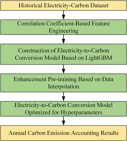
Based on the analysis above, optimizing the hyperparameters of machine learning algorithms under small-sample conditions is a critical step to improving accounting accuracy. To address this, we propose an “electricity-to-carbon conversion” method based on electricity data and augmentation pre-training, as outlined in Figure 1. This approach consists of three main steps: feature engineering, model construction, and augmentation pre-training.

Figure 1

Figure 1. Overall framework of the proposed method.

First, feature engineering involves analyzing the correlation between collected electricity production and consumption data and carbon emissions data to select highly correlated electricity data as input features for the “electricity-to-carbon conversion” model. Second, an appropriate machine learning algorithm is chosen to build the model, mapping the input features to annual carbon emissions. Finally, to optimize the model under small-sample conditions, we introduce an augmentation pre-training optimization method to obtain the optimal hyperparameters for the “electricity-to-carbon conversion” model.

3 Methodology overview

The following sections provide a detailed introduction to each component of the proposed framework.

3.1 Feature engineering

The “electricity-to-carbon conversion” method relies on the correlation between electricity and carbon emission data. Therefore, it is essential to perform correlation analysis on the collected power generation and consumption data, selecting the electricity data most strongly correlated with carbon emissions as input features for the model.

In this study, the Pearson correlation coefficient and Spearman correlation coefficient are used to quantify the relationship between feature data and target data (Cohen et al., 2009). Their calculations are shown in Equations 2, 3:

$R_p=\frac{{\displaystyle \sum _{i=1}^n}\left(x_i-\overline{x}\right)\left(y_i-\overline{y}\right)}{\sqrt{{\displaystyle \sum _{i=1}^n}{\left(x_i-\overline{x}\right)}^2{\displaystyle \sum _{i=1}^n}\left(y_i-\overline{y}\right)}}(2)$

$R_s=1-\frac{6{\displaystyle \sum _{i=1}^n}{d_i}^2}{n\left(n^2-1\right)}(3)$

Where $R_p$ denotes the Pearson correlation coefficient and $R_s$ denotes the Spearman correlation coefficient. $x_i$ and $y_i$ denote the values of the two variables for the $i$-th sample point, while $\overline{x}$ and $\overline{y}$ are the means of the two variables. The variable $d_i$ denotes the difference in ranks between $x_i$ and $y_i$, and $n$ represents the sample size.

The Spearman and Pearson correlation coefficients are used to assess the relationship between feature data and target data, with values ranging from −1 to 1. A value closer to 0 indicates a weaker correlation, while values closer to 1 signify a stronger positive correlation, and values closer to −1 indicate a stronger negative correlation. The Spearman coefficient measures monotonic relationships without requiring linearity or normal distribution of the data, whereas the Pearson coefficient reflects only linear correlations and assumes that the data follows a normal distribution (Hauke and Kossowski, 2011).

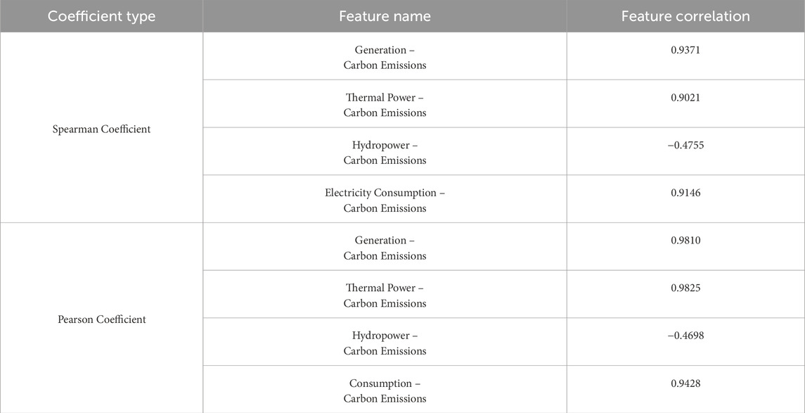
Data from the past 17 years (2004–2021) were used in the calculation and Table 1 presents the correlation analysis results between various electricity data and carbon emissions. The data reveals a strong monotonic and linear relationship between total annual carbon emissions and electricity consumption, thermal power generation, and total electricity, while a negative correlation is observed with hydropower generation. Therefore, electricity data, excluding hydropower generation, is selected as input variables for the model.

Table 1

Table 1. Correlation coefficients between various electricity data and carbon emissions.

3.2 “Electricity-to-carbon conversion” model

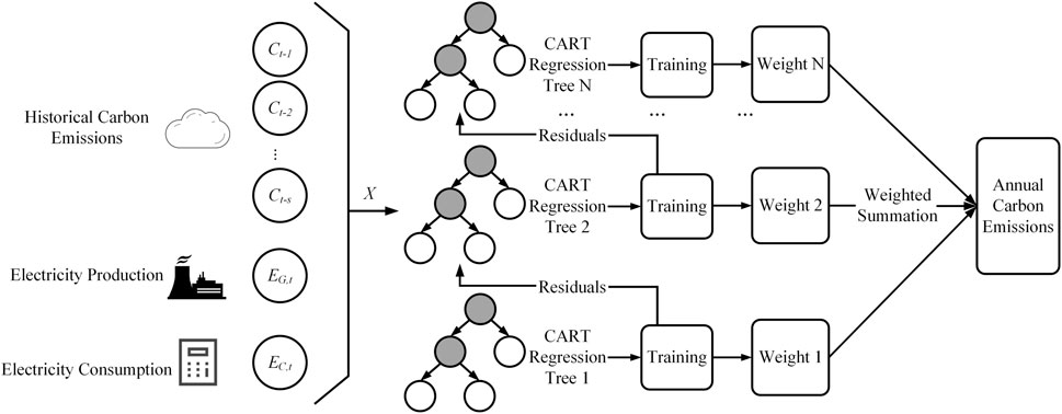
Figure 2 illustrates the structure of the proposed “electricity-to-carbon conversion” model. The input variables $X$ include this year’s electricity production $P_{G,t}$ (comprising total generation and thermal power generation), historical carbon emissions $C_{t-1},C_{t-2},\cdots C_{t-s}$, and total electricity consumption $P_{C,t}$. The composition of the input variable X is shown in Equation 4:

$X=\left\{X_1,X_2\cdots X_n\right\}=\left\{C_{t-1},C_{t-2}\cdots C_{t-s},P_{G,t},P_{C,t}\right\}(4)$

Figure 2

Figure 2. Structure of the “electricity-to-carbon conversion” model.

This study employs the Light Gradient Boosting Machine (LightGBM) as the regression fitting model. LightGBM is a machine learning algorithm based on decision tree methods and gradient boosting, designed to iteratively optimize model residuals and enhance predictive performance (Wang et al., 2017; Ke et al., 2017). Comprising multiple simple decision trees, LightGBM features a simpler structure compared to other machine learning models, making it particularly suitable for small sample learning tasks. Additionally, it utilizes methods such as histogram algorithms and leaf-wise strategies to improve computational efficiency and predictive accuracy. The mathematical model for LightGBM is expressed in Equation 5:

${\mathit{C}}_t={\displaystyle \sum _{n=1}^N}{f}_n\left(d_t\right)(5)$

where ${\mathit{C}}_t$ denotes the estimated annual carbon emissions obtained from the LightGBM model; $f_n\left(d_t\right)$ denotes the estimate from the n-th regression tree; t represents time; N indicates the total number of regression trees; and n denotes the specific tree number.

The objective function of the LightGBM model comprises a loss function and a regularization term. The expression for the objective function of the t-th tree is provided in where Equation 6. The expressions for the loss function and the regularization penalty are given in where Equation 7 and where Equation 8, respectively.

$Y_n=L_n+{\mathrm{\Omega }}_n(6)$

$L_n={{\displaystyle \sum _{t=1}^T}\left[C_t-\left({\mathit{C}}_t^{n-1}+f_n\left(d_t\right)\right)\right]}^2(7)$

${\mathrm{\Omega }}_n=\gamma J+\frac{1}{2}\lambda {\displaystyle \sum _{j=1}^J}{w}_j^2(8)$

where $Y_n$ denotes the objective function of the n-th tree, and $L_n$ and ${\mathrm{\Omega }}_n$ represent the loss function and regularization penalty of the n-th tree, respectively. J denotes the number of leaf nodes, while w signifies the weight values of these nodes. j refers to the j-th leaf node, and λ represents the penalty coefficient for the leaf nodes. T denotes the total number of samples, and ${\mathit{C}}_t^{n-1}$ indicates the estimate of the i-th sample from the n−1-th tree.

The input variable X and annual carbon emissions Y are designated as the feature set and target set, respectively, for training the LightGBM model. The final LightGBM model is obtained after multiple iterations, converging to the minimum loss.

3.3 Model optimization method based on augmentation pre-training

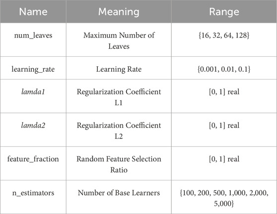
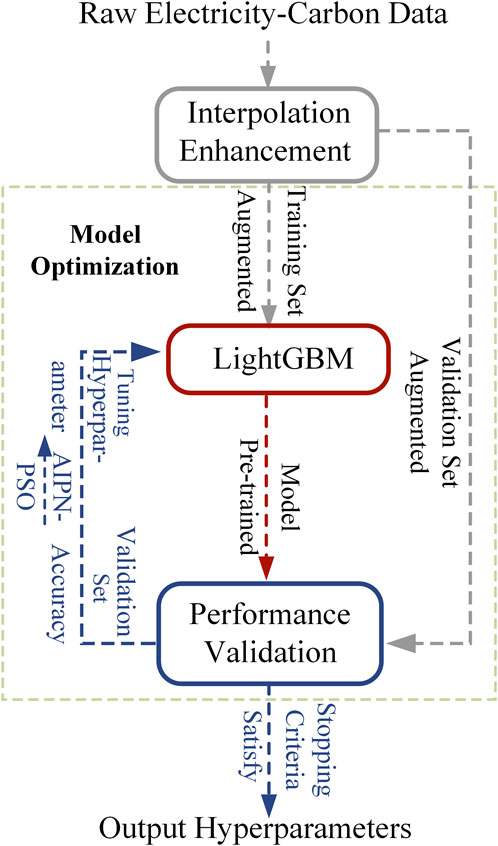
The hyperparameters required for LightGBM are shown in Table 2. The selected hyperparameters have a direct and significant impact on the model’s fitting performance. To ensure that the “electricity-to-carbon conversion” model has good generalization performance and regression fitting ability, effective optimization of the hyperparameters is necessary. However, in cases with insufficient sample sizes, model optimization can easily fall into local optima. To enable more thorough and effective optimization under small sample conditions, this paper proposes a model optimization method based on augmentation pre-training. Figure 3 illustrates the processing flow of the augmentation pre-training method, which generates a large amount of augmented data through an interpolation augmentation module, allowing the LightGBM model to undergo pre-training and optimization on this augmented dataset to obtain a set of optimal hyperparameters for formal training.

Table 2

Table 2. Hyperparameters to be determined in the LightGBM model.

Figure 3

Figure 3. Augmentation pre-training flowchart.

Interpolation augmentation is the primary step of augmentation pre-training. As shown in Figure 4, this method first uses numerical interpolation to fit discrete data points into a continuous numerical function $y\left(t\right)$ and then performs high-frequency sampling on this function to obtain a large amount of augmented data. In the interpolation method, the commonly used piecewise linear interpolation approximates $y\left(t\right)$ by connecting adjacent interpolation points with line segments. Its mathematical modeling is represented by Equations 9, 10:

$y_h\left(t\right)={\displaystyle \sum _{j=0}^n}{y}_j{l}_j\left(t\right)(9)$

$l_j\left(t\right)=\left\{\begin{array}{l}\frac{t-t_{j-1}}{t_j-t_{j-1}},t_{j-1}\le t\le t_j,\left(j\ne 0\right)\\ \frac{t-t_{j+1}}{t_j-t_{j+1}},t_j\le t\le t_{j+1},\left(j\ne n\right)\\ 0,t\notin \left[t_{j-1},t_{j+1}\right]\end{array}\right.(10)$

Figure 4

Figure 4. Interpolation augmentation flowchart.

Where, t represents time, serving as the independent variable for the fitted function $y_h\left(t\right)$, while $l_j\left(t\right)$ represents the interpolation basis function. $t_j$ and $y_j$ denote the j-th group of sampling points in the dataset.

Assuming that when $y\left(t\right)\in C^2\left[t_1,t_2\right]$ is given, there exists an upper bound on the error between the piecewise linear interpolation function $y_h\left(t\right)$ and the actual function $y\left(t\right)$. The upper bound of the error, $\underset{t_1\le t\le t_n}{\max }\left|y\left(t\right)-y_h\left(t\right)\right|$, can be estimated using Equation 11.

$\underset{t_1\le t\le t_n}{\max }\left|y\left(t\right)-y_h\left(t\right)\right|=\frac{\underset{t_1\le t\le t_n}{\max }\left|y^{″}\left(t\right)\right|}{8}{h}^2(11)$

Where, h denotes the sampling interval, i.e., $h=t_j-t_{j-1},j\ne 0$. As indicated by Equation 11, there exists an upper limit on the error between the augmented data and the real data, which ensures the reliability of the numerical augmentation method.

Model optimization is the core step of augmentation pre-training, achieved through an iterative process of “training-evaluation-feedback” adjustment for hyperparameter optimization. In each iteration, the LightGBM is first trained on the augmented training set, then the fitting performance is evaluated on the augmented validation set, and finally, hyperparameters are optimized based on the evaluation results.

To efficiently optimize hyperparameters in a complex parameter space, this study proposes an improved particle swarm optimization algorithm based on adaptive inertia weight and local neighborhood strategy (Adaptive Inertia and Local Neighborhood Particle Swarm Optimization, AILN-PSO). The PSO algorithm is a classic swarm intelligence optimization method that effectively addresses continuous optimization problems but suffers from low computational efficiency and a tendency to fall into local optima (Marini and Walczak, 2015). Therefore, we employ adaptive inertia weights and local neighborhood strategies to enhance the algorithm’s computational efficiency and optimization accuracy.

In standard PSO, the inertia weight controls the search step of the particles. When the weight is large, particles tend to explore a larger search space; when the weight is small, particles focus more on local searches. The adaptive inertia weight dynamically balances exploration and exploitation by adjusting the weight value at different stages of the algorithm. To improve efficiency, this study adjusts the inertia weight to a function that decreases as the number of iterations increases, allowing the search to transition from global to local. The expression for the adaptive inertia weight is shown in Equation 12.

$\omega \left(k\right)={\omega }_{\max }-\left(\frac{{\omega }_{\max }-{\omega }_{\min }}{K_{\max }}\right)\times k(12)$

Where, ${\omega }_{\max }$ and ${\omega }_{\min }$ denote the maximum and minimum values of the inertia weight, respectively, while $K_{\max }$ denotes the maximum number of iterations, and k is the current iteration count.

In standard PSO, all particles update their positions based on the global best particle. However, the global best particle may sometimes limit the particles’ ability to escape local optima. The local neighborhood strategy enhances the diversity of the population by allowing each particle to update its position based only on the best particle in its neighborhood, which helps to avoid getting trapped in local optima. Under this strategy, the update velocity and position of the particles are represented by Equations 13, 14, respectively.

$v_a\left(k+1\right)=\omega \left(k\right)\cdot v_a\left(k\right)+c_1\cdot r_1\cdot \left(p_a\left(k\right)-x_a\left(k\right)\right)+c_2\cdot r_2\cdot \left(l_a\left(k\right)-x_a\left(k\right)\right)(13)$

$x_a\left(k+1\right)=x_a\left(k\right)+v_a\left(k+1\right)(14)$

Where, $x_a\left(k\right)$ and $v_a\left(k\right)$ represent the position and velocity of particle A at the k-th iteration, while $c_1$ and $c_2$ are the acceleration coefficients. $r_1$ and $r_2$ are random numbers. $p_a\left(k\right)$ denotes the historical best position of particle a and $l_a\left(k\right)$ indicates the best position of particle A within its local neighborhood. In this study, the Mean Squared Error (MSE) of the pre-trained model on the augmented validation set is used as the evaluation metric. The maximum number of iterations for AILN-PSO is set to 300, and an early stopping mechanism is implemented. Specifically, if the evaluation value does not improve for 10 consecutive iterations, it is considered that the optimization process has converged, leading to the termination of training and the output of the optimized hyperparameters.

4 Case analysis

4.1 Experimental data

The carbon emission dataset used in this study is sourced from the China Carbon Accounting Database (CEADs) (Shan et al., 2018; Shan et al., 2020; Xu et al., 2024), while the electricity data comes from the National Bureau of Statistics (National Bureau of Statistics of China, 2024). The electricity data includes electricity consumption, total power generation, thermal power generation, and hydropower generation. The dataset spans from 1997 to 2021, with an annual granularity.

4.2 Experimental setup

To comprehensively evaluate the performance of the proposed method, various machine learning models suitable for small sample learning were selected for comparison. The specific models are as follows:

1) ARMA: The Auto-Regressive Moving Average (ARMA) model is a commonly used time series model that extrapolates future data points based on past time series. ARMA uses only historical carbon emissions as input data and does not include electricity data.

2) MLP: The Multilayer Perceptron (MLP) is a type of feedforward neural network trained using the backpropagation algorithm. MLP can handle complex nonlinear problems and is widely used in regression tasks, but it has many hyperparameters that require careful selection of model structure.

3) SVM: The Support Vector Machine (SVM) effectively addresses nonlinear regression problems through kernel functions and helps prevent overfitting, thus maintaining good generalization capabilities with small samples. Given its potential advantages in small sample learning, it is selected as the benchmark model.

The length of historical data has a critical impact on model performance: an appropriate historical data length allows the model to capture and learn the changing trends in carbon emissions, while a length that is too long increases feature complexity and reduces the amount of training samples. Therefore, this study first discusses the selection of historical data length by comparing the performance of models with different historical data lengths to determine the optimal length.

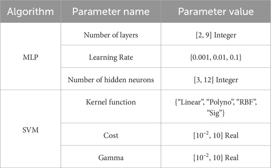
Table 3 presents the hyperparameters to be optimized of MLP and SVM model. To validate the effectiveness of the proposed augmentation pre-training method in small sample learning, the hyperparameter optimization method based on augmentation pre-training is compared with the hyperparameter optimization method using the validation set. In augmentation pre-training optimization, the model’s hyperparameter optimization is conducted on the augmented dataset; whereas in validation set optimization, the hyperparameters are optimized on the validation set. In both methods, the dataset is divided into training, validation, and test sets, with proportions of 6:2:2.

Table 3

Table 3. Hyperparameters of MLP and SVM model.

4.3 Evaluation metrics

This study employs two statistical metrics to assess the goodness of fit of the “electricity-to-carbon conversion” model: Mean Absolute Percentage Error (MAPE) and Root-Mean-Square Error (RMSE). These two metrics are commonly used in regression analysis, with smaller values indicating less deviation between the fitted values and the actual values. RMSE is an error evaluation metric that measures the deviation between predicted values and target values, with smaller numbers indicating closer alignment between model predictions and target values. MAPE is a relative error evaluation metric suitable for comparing the error rates between different model predictions and target values, where smaller values signify lower errors. Their expressions are given in Equations 15, 16:

$RMSE=\sqrt{\frac{1}{n}{\displaystyle \sum _{i=1}^n}{\left({\widehat{y}}_i-y_i\right)}^2}(15)$

$MAPE=\frac{100\%}{n}{\displaystyle \sum _{i=1}^n}\left|\frac{{\widehat{y}}_i-y_i}{y_i}\right|(16)$

Where, ${\mathit{y}}_i$ denotes the i-th output value of the model, $y_i$ denotes the actual value at the i-th point, and n indicates the number of samples.

4.4 Experimental results and analysis

The accounting results of carbon emissions are shown in Tables 4, 5.

Table 4

Table 4. MAPE of each accounting method.

Table 5

Table 5. RMSE of each accounting method.

Tables 4, 5 present the performance evaluation data of each model under different historical data lengths, revealing significant differences in performance across methods. Shorter data lengths provide better accounting accuracy due to the availability of more training samples and the substantial variations in carbon emission trends over different periods. Additionally, each machine learning model achieved better results using the augmentation pre-training optimization method.

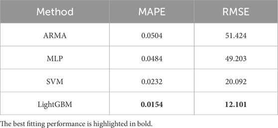
A comparison of the models under the optimal method is shown in Table 6, detailing their fitting performance. It is evident from the table that all models outperform ARMA, which relies solely on the autocorrelation characteristics of historical carbon emissions without incorporating power features. This indicates that power features significantly enhance accounting accuracy. For MLP, the training data volume is still too limited, hindering its learning effectiveness. SVM and LightGBM show good accounting results, demonstrating their superiority in small sample learning tasks. LightGBM, with its simpler structure, more easily identifies suitable hyperparameters, yielding good fitting performance under both optimization methods. In contrast, SVM has numerous and complex hyperparameters that require richer samples for optimization, resulting in suboptimal performance on the small sample validation set, although significant accuracy improvements were observed after augmentation pre-training optimization.

Table 6

Table 6. Comparison of fitting errors of each model under optimal parameters.

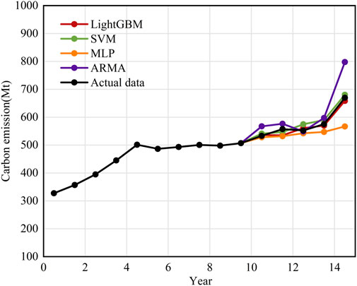
To provide a more intuitive comparison of the differences between the various models’ “electricity-to-carbon” performance, the accounting results of all models utilizing the best method on the test set are compared with the actual values, as shown in Figure 5 and Table 7.

Figure 5

Figure 5. Accounting results of different models.

Table 7

Table 7. Estimation results of each model.

From the analysis of Figure 5, it is evident that ARMA and MLP exhibit significant deviations between their measured values and target values, with some accountings being either too high or too low. Although the SVM regression model shows better evaluation results, there remains a noticeable deviation between many fitted values and the target values. In contrast, LightGBM’s fitted values align more closely with the target values, demonstrating a tighter distribution of accounting values relative to the actual target values.

5 Conclusion

To address the challenges of using machine learning methods for “electricity-to-carbon” conversion in small samples, this paper proposes a novel approach based on augmentation pre-training. Specifically, the proposed method generates a substantial amount of augmented data through interpolation augmentation for model pre-training, optimizing and determining the model’s hyperparameters in the process. The pre-trained hyperparameters are then retained and applied to the formal training, thereby overcoming the difficulties in optimizing machine learning models under small sample conditions and improving model performance.

To validate the effectiveness of the proposed method, common time series models such as ARMA, SVM, and MLP were selected as benchmark models for comparative experiments. The experimental results indicate that the proposed method significantly enhances the accuracy of carbon emission accountings under small sample conditions when compared to various benchmark methods, providing a feasible solution for rapid, precise, and low-cost annual carbon emission accounting.

There are still some limitations in the current work, which will be addressed in future studies. For instance, the current research lacks an in-depth exploration of the authenticity of the augmented data and its impact on model performance. Future research should focus on the influence of interpolation augmentation methods on augmentation pre-training. Additionally, the carbon emission accounting method proposed in this study has only been tested on annual datasets, so its effectiveness and generalizability on high-resolution datasets also require significant investigation.

Data availability statement

The data analyzed in this study is subject to the following licenses/restrictions: None. Requests to access these datasets should be directed to HF, 969082563@qq.com.

Author contributions

BP: Writing–review and editing, Writing–original draft. YL: Writing–review and editing, Visualization, Validation, Supervision, Software, Resources, Project administration, Methodology, Investigation, Funding acquisition, Formal Analysis, Data curation, Conceptualization. CY: Writing–original draft, Validation, Supervision, Methodology. HF: Writing–review and editing, Conceptualization, Validation, Project administration, Formal Analysis. XG: Writing–review and editing, Visualization, Formal Analysis.

Funding

The author(s) declare that financial support was received for the research, authorship, and/or publication of this article. This work is funded by the Planning Thematic Project of China Southern Power Grid, Project Name: Research on dynamic monitoring technology for carbon emissions of key energy consuming enterprises and carbon coupling mechanism of power transmission network, Grant No. 031000QQ00230001.

Conflict of interest

Authors BP, YL, and XG were employed by Guangdong Power Grid Corporation.

The remaining authors declare that the research was conducted in the absence of any commercial or financial relationships that could be construed as a potential conflict of interest.

Generative AI statement

The author(s) declare that no Generative AI was used in the creation of this manuscript.

Publisher’s note

All claims expressed in this article are solely those of the authors and do not necessarily represent those of their affiliated organizations, or those of the publisher, the editors and the reviewers. Any product that may be evaluated in this article, or claim that may be made by its manufacturer, is not guaranteed or endorsed by the publisher.

References

Aras, S., and Van, M. H. (2022). An interpretable forecasting framework for energy consumption and CO2 emissions. Appl. Energy 328, 120163. doi:10.1016/j.apenergy.2022.120163

CrossRef Full Text | Google Scholar

Chaudhari, A., and Mulay, P. (2019). Algorithmic analysis of intelligent electricity meter data for reduction of energy consumption and carbon emission. Electr. J. 32 (10), 106674. doi:10.1016/j.tej.2019.106674

CrossRef Full Text | Google Scholar

Cohen, I., Benesty, J., Chen, J., and Huang, Y. (2009). “Pearson correlation coefficient,” in Noise reduction in speech processing, 1–4.

CrossRef Full Text | Google Scholar

Hauke, J., and Kossowski, T. (2011). Comparison of values of Pearson's and Spearman's correlation coefficients on the same sets of data. Quaest. Geogr. 30 (2), 87–93. doi:10.2478/v10117-011-0021-1

CrossRef Full Text | Google Scholar

Huang, C., Li, K., and Zhang, N. (2025). Strategic joint bidding and pricing of load aggregators in day-ahead demand response market. Appl. Energy 377, 124552. doi:10.1016/j.apenergy.2024.124552

CrossRef Full Text | Google Scholar

IEA (2023). CO2 emissions in 2022 – analysis. Available at: https://www.iea.org/reports/co2-emissions-in-2022 (Accessed August 14, 2024).

Google Scholar

Jiang, T., Yu, Y., and Jahanger, D, A. (2022). Balsalobre-Lorente, Structural emissions reduction of China’s power and heating industry under the goal of ‘double carbon’: a perspective from input-output analysis. Sustain Prod. Consum. 31, 346–356. doi:10.1016/j.spc.2022.03.003

CrossRef Full Text | Google Scholar

Ke, G., Meng, Q., Finley, T., Wang, T., Chen, W., Ma, W., et al. (2017). LightGBM: a highly efficient gradient boosting decision tree. Adv. Neural Inf. Process. Syst. 30, 52.

Google Scholar

Kim, J., Seo, B. K., Lee, T., Kim, J., Kim, S., Bae, G. N., et al. (2023). Airborne estimation of SO 2 emissions rates from a coal-fired power plant using two top-down methods: a mass balance model and Gaussian footprint approach. Sci. Total Environ. 855, 158826. doi:10.1016/j.scitotenv.2022.158826

PubMed Abstract | CrossRef Full Text | Google Scholar

Li, K., Li, Z., Huang, C., and Ai, Q. (2024). Online transfer learning-based residential demand response potential forecasting for load aggregator. Appl. Energy 358, 122631. doi:10.1016/j.apenergy.2024.122631

CrossRef Full Text | Google Scholar

Li, M., Wang, W., De, G., Ji, X., and Tan, Z. (2018). Forecasting carbon emissions related to energy consumption in Beijing-Tianjin-Hebei region based on grey prediction theory and extreme learning machine optimized by support vector machine algorithm. Energies 11 (9), 2475. doi:10.3390/en11092475

CrossRef Full Text | Google Scholar

Marini, F., and Walczak, B. (2015). Particle swarm optimization (PSO). A tutorial. Chemom. Intelligent Laboratory Syst. 149, 153–165. doi:10.1016/j.chemolab.2015.08.020

CrossRef Full Text | Google Scholar

National Bureau of Statistics of China (2024). Data query. Available at: https://data.stats.gov.cn/search.

Google Scholar

Shan, Y., Guan, D., Zheng, H., Ou, J., Li, Y., Meng, J., et al. (2018). China CO2 emission accounts 1997–2015. Sci. Data 5, 170201. doi:10.1038/sdata.2017.201

PubMed Abstract | CrossRef Full Text | Google Scholar

Shan, Y., Huang, Q., Guan, D., and Hubacek, K. (2020). China CO2 emission accounts 2016–2017. Sci. Data 7, 54. doi:10.1038/s41597-020-0393-y

PubMed Abstract | CrossRef Full Text | Google Scholar

Wang, D., Zhang, Y., and Zhao, Y. (2017). “LightGBM: an effective miRNA classification method in breast cancer patients,” in Proc. 2017 int. Conf. Comput. Biol. Bioinformatics, 7–11.

CrossRef Full Text | Google Scholar

Wang, Q., Huang, C., Wang, C., Li, K., and Xie, N. (2024). Joint optimization of bidding and pricing strategy for electric vehicle aggregator considering multi-agent interactions. Appl. Energy 360, 122810. doi:10.1016/j.apenergy.2024.122810

CrossRef Full Text | Google Scholar

Xu, J. H., Guan, Y. R., Oldfield, J., Guan, D., and Shan, Y. (2024). China carbon emission accounts 2020-2021. Appl. Energy 360, 122837. doi:10.1016/j.apenergy.2024.122837

CrossRef Full Text | Google Scholar

Zhang, X., Zhang, H., Zhao, C., and Yuan, J. (2019). Carbon emission intensity of electricity generation in Belt and Road Initiative countries: a benchmarking analysis. Environ. Sci. Pollut. Res. 26, 15057–15068. doi:10.1007/s11356-019-04860-5

PubMed Abstract | CrossRef Full Text | Google Scholar

Zubair, M., Chen, S., Ma, Y., and Hu, X. (2023). A systematic review on carbon dioxide (CO2) emission measurement methods under PRISMA guidelines: transportation sustainability and development programs. Sustainability 15, 4817. doi:10.3390/su15064817

CrossRef Full Text | Google Scholar