A comparative study of different deep learning methods for time-series probabilistic residential load power forecasting

The widespread adoption of nonlinear power electronic devices in residential settings has significantly increased the stochasticity and uncertainty of power systems. The original load power data, characterized by numerous irregular, random, and probabilistic components, adversely impacts the predictive performance of deep learning techniques, particularly neural networks. To address this challenge, this paper proposes a time-series probabilistic load power prediction technique based on the mature neural network point prediction technique, i.e., decomposing the load power data into deterministic and stochastic components. The deterministic component is predicted using deep learning neural network technology, the stochastic component is fitted with Gaussian mixture distribution model and the parameters are fitted using great expectation algorithm, after which the stochastic component prediction data is obtained using the stochastic component generation method. Using a mature neural network point prediction technique, the study evaluates six different deep learning methods to forecast residential load power. By comparing the prediction errors of these methods, the optimal model is identified, leading to a substantial improvement in prediction accuracy.

1 Introduction

To achieve China’s dual-carbon goals of reaching carbon peaking by 2030 and carbon neutrality by 2060, we need accurate load power forecasts (Huang et al., 2024). In addition, precise load power predictions can greatly reduce power system operating costs. However, access to a large number of distributed power sources, including electric vehicles, has greatly increased the stochasticity and uncertainty of the power system, presenting new challenges to load power forecasting. Reliable load forecasting is essential for risk management and is a fundamental task for system operation and planning.

An important aspect of load power forecasting is analyzing the factors affecting load power. Mathematical models have been developed to capture the intrinsic relationship between influencing factors and load variations. For example, a learning prediction method for deep transfer of power zoning considering the matching of contact line characteristics is proposed in (Li JF. et al., 2023). In (Yudantaka et al., 2020), to improve the accuracy of load power prediction, a Long Short-Term Memory (LSTM) network is trained using past temperature and load power data. To address excessive temperature prediction errors, past data describing the relationship between temperature changes and load power variations are used to train a multilayer perceptron network (Wang K. et al., 2024). The results show that the proposed compensation using real-time temperature information improves the performance of load power prediction. In (Liao et al., 2022), to cope with the volatility and stochasticity of power loads, a new deep generative network-based power load scenario prediction method is proposed, where the structure and parameters are redesigned based on the original pixel convolutional neural network to enhance the prediction accuracy. In (Xia et al., 2023), an improved fuzzy support vector regression machine method for power load forecasting is proposed, using boundary vector extraction to improve the accuracy and speed of power load forecasting.

In recent years, researchers around the globe have made significant progress in power load forecasting. Commonly used prediction models include artificial neural networks, support vector machines, and extreme learning machines, among others. In (Cui et al., 2020), an LSTM prediction model for load forecasting is established based on the time series behavior of power load, improving prediction accuracy. A prediction model based on CEEMDAN is proposed in (Huang et al., 2020), effectively overcoming the problem of EMD modal aliasing, leading to a more complete decomposition process and improved prediction accuracy. In (Lu et al., 2019), the stability of the GM model, widely used in load forecasting, is highlighted along with the detailed constraints leading to model instability. In (Gao, 2019), a multivariate grey theoretical prediction model is proposed, with multivariate residual error correction significantly enhancing prediction accuracy. In (Wu, 2017), grey forecasting is studied in depth, demonstrating good adaptability to medium- and long-term power loads. In (Yao et al., 2022), a short-term power load prediction model based on feature selection and error correction is proposed to address the problem of low accuracy and weak generalization ability in short-term power load prediction. In (Sun and Cai, 2022), a short-term power load forecasting model based on variational mode decomposition is proposed, exhibiting high fitting ability and forecasting accuracy, making it an effective short-term load forecasting method. In (Wang et al., 2020) and (Ning et al., 2021), the particle swarm algorithm is employed to improve the prediction model, further enhancing prediction accuracy.

As load data incorporates increasingly complex factors, traditional single models struggle to fully explore the intrinsic information within the data. However, hybrid prediction models can address the shortcomings of single prediction methods, offering better stability and accuracy. A hybrid algorithm based on wavelet transform and support vector machine is proposed in (Jin et al., 2020) to improve load forecasting accuracy. An approach combining fuzzy support vector machine and grey prediction is proposed in (Xiong et al., 2022; Gao et al., 2024), significantly improving prediction accuracy. In (Li et al., 2024), a new method for power load forecasting that combines grey correlation-oriented random forest and quasi-tidal swarm optimization algorithm is proposed, further improving forecasting accuracy. In (Wang ZX. et al., 2024; Zou and Tao, 2014; Chen et al., 2024), a hybrid prediction method based on a support vector machine is proposed, which is combined with an adaptive evolutionary learning machine, wavelet transform, and grey combinatorial prediction, respectively, to improve the accuracy of prediction. Based on the variational modal decomposition technique (Zhang et al., 2023; Cao et al., 2023), combines multiple prediction methods, which not only improves the prediction accuracy, but also improves the stability of the prediction model.

In conclusion, hybrid prediction models offer great advantages and development potential over single prediction models. In this paper, a new hybrid forecasting model is proposed. Residential load power is decomposed into deterministic and stochastic components, which are then predicted separately. For the deterministic component, various neural network-based methods are utilized to predict multiple steps, and the best prediction method is selected based on prediction error. For the stochastic component, the method of probabilistic prediction is adopted, where a Gaussian mixture model (GMM) is established to fit the probability density function of each period of the day using multiple Gaussian functions, serving as the probabilistic prediction result of the stochastic component (Xie et al., 2024a). The optimal parameters of the model are determined using the Expectation Maximization (EM) algorithm. To test the accuracy of the prediction results, the stochastic component generation method is employed to draw random samples from the probabilistic prediction results, simulate the predicted values of the stochastic component, and compare them with the actual residential load power by adding them to the point prediction results of the deterministic component, thereby calculating the prediction error and testing the effectiveness of the prediction model. Finally, to prove the practicality of the prediction model established in this paper, the optimal neural network selected is used to perform point prediction on the same dataset, which is then compared with the time-series probabilistic prediction model established in this paper.

The second section of this paper characterizes the residential load and separates the deterministic and stochastic components. The third section describes various neural network prediction methods for the deterministic component and prediction methods for the stochastic component. The fourth section presents the simulation analysis, and the fifth section concludes the study.

2 Processing and characterization of residential load power data

2.1 Characterization of residential loads

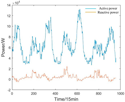
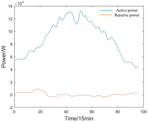
The waveform of residential load power contains a wealth of information and fully exploring its underlying patterns can significantly enhance our ability to predict residential load power. Figure 1 illustrates the variation of residential load power over a 10-day period, while Figure 2 shows the changes in residential load power over a single day, with time intervals of 15 min.

Figure 1

Figure 1. Overview of residential load power time series over a 10-day period.

Figure 2

Figure 2. Overview of the residential load power time series over a day.

Based on these figures and the actual conditions, we can identify three key characteristics of residential load power: randomness, periodicity, and diversity.

• Firstly, the trend in residential load power data is typically influenced by the type and number of electrical appliances used by the residents. The power consumption of different appliances varies, and while there may be a general pattern in terms of when certain appliances are used, the presence of uncertainty factors can cause abnormal fluctuations in load power, which in turn affects prediction accuracy.

• Secondly, residential load power data is closely linked to people’s daily routines. The repetition of daily and weekly activities leads to regular changes in load power data, which reflect these recurring patterns.

• Finally, there are significant variations in residential load power data across different regions. A prediction method that performs well on one dataset may result in substantial errors when applied to another dataset. Therefore, it is essential to analyze specific cases and select the prediction method that best suits the characteristics of the dataset to achieve optimal prediction results.

2.2 Separation of deterministic and stochastic components

As residential load power is characterized by randomness, dispersion, periodicity, and diversity, these characteristics cause residential load power to exhibit two patterns of change over time: deterministic and stochastic. To better predict the residential load power, this paper separates residential load power into deterministic components and stochastic components, i.e, Equation 1, with point prediction for the deterministic component and probabilistic prediction for the stochastic component (Li YH. et al., 2023).

$P=P_{certain}+P_{random}(1)$

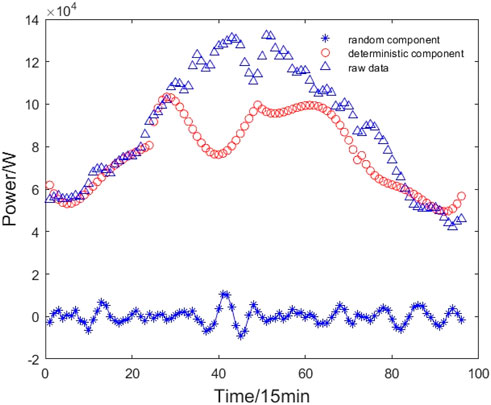
There are many methods to achieve the separation of deterministic and stochastic components in time series, such as the moving average method, exponential smoothing, and polynomial fitting (Zhang et al., 2024). Due to the large fluctuations in residential load data, the weighted moving average method was chosen to achieve the separation of the deterministic and stochastic components. Weighted moving average is a method of data smoothing that gives unequal weights to each variable value over a fixed period. The principle is that historical data are not equally useful for predicting future data. Figure 3 shows the decomposition effect of residential load power.

Figure 3

Figure 3. Decomposition of residential load power data during a day.

As seen in Figure 3, the deterministic component is the most important part, and its time series is smooth and stable, representing the sequential change pattern of residential load power. In contrast, the stochastic component is similar to the noise, with a small amplitude, and its time series fluctuates above and below the zero value without any regularity, reflecting the volatility of residential load power.

3 Time-series probabilistic residential load power prediction

3.1 Neural network-based power prediction for time-series residential loads

A neural network is a computer algorithm, also known as an artificial neural network, that is inspired by the process of information processing in the brains of humans and animals (Sun et al., 2021). This section introduces the fundamentals of six types of neural networks: multilayer perceptron (MLP) networks, convolutional neural network (CNN), recurrent neural network (RNN), LSTM neural networks, bidirectional LSTM (Bi-LSTM) neural networks, and encoder and decoder LSTM (ED-LSTM) neural networks, which will be covered in the next six subsections.

3.1.1 MLP networks

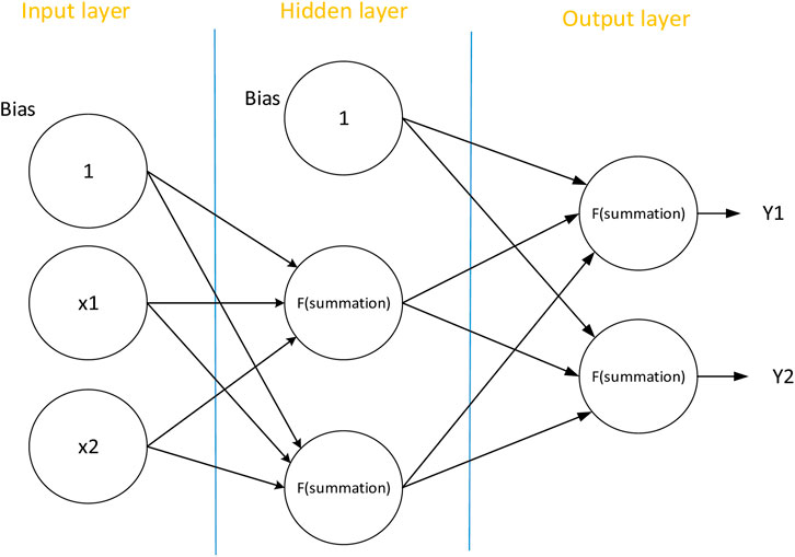
MLP, also known as a feed-forward neural network, is the simplest shallow neural network. It has only one input layer and one output layer, while the hidden layer can have one or more layers, enabling it to learn nonlinear functions. The connections between the different layers of an MLP network are fully connected, and the basic structure of an MLP containing one hidden layer is shown in Figure 4.

Figure 4

Figure 4. MLP basic structure.

3.1.2 CNN

A CNN is a type of forward neural network that has been widely used in the fields of computer vision and time series analysis and is one of the most basic and important components of deep learning. Because CNNs are locally connected and share weights, they can effectively reduce both error decay and training weights, thereby reducing the complexity of the network and improving the model’s feature mapping ability compared with general neural networks. The structure of a CNN is shown in Figure 5.

Figure 5

Figure 5. Structure of CNN.

The most important components in the CNN network structure are the convolutional layer and the pooling layer. Each neuron in the convolutional layer is interconnected with the localized feature region of the previous layer through the convolution kernel, and the convolutional layer extracts different features of different time series data through such convolution operations. The role of the pooling layer is to further extract the features of the data to reduce the dimensionality of the data. The commonly used pooling methods are the maximum pooling method, mean pooling method, and so on.

For time-series data, a one-dimensional CNN is used. When the lth layer of the CNN is a convolutional layer, the one-dimensional convolution is calculated as Equation 2:

$x_k^l=f\left({\displaystyle \sum _{i=1}^N}{x}_i^{l-1}\otimes w_{ik}^l+b_k^l\right)(2)$

where $x_k^l$ is the kth convolutional mapping of layer l; f is the activation function; N is the number of inputs performing convolutional mapping; $\otimes$ is the convolutional operation; $w_{ik}^l$ is the weight of the kth convolution kernel of layer l performing the ith operation; $b_k^l$ is the bias of the kth convolution kernel corresponding to layer l.

For the pooling layer, in this paper, the maximum pooling method is used, and Equation 3 represents taking the maximum value from vector $x_k^l$ to $x_{k+r-1}^l$. For the sequence x, the maximum pooling operation is repeated for each consecutive vector with window r to obtain the largest feature sequence.

${\stackrel{\sim }{x}}_k^l=\max \left(x_k^l:x_{k+r-1}^l\right)(3)$

3.1.3 RNN

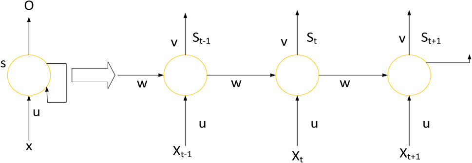
The RNN was first proposed in the 1980s. An RNN connects neurons in series, allowing each neuron to have a certain degree of memory and store the information from previous input sequences. Additionally, the RNN parameters can be shared, and it exhibits strong learning abilities for nonlinear time series, making it an effective tool for time series analysis. The network structure of an RNN is shown in Figure 6.

Figure 6

Figure 6. RNN structure.

The network function of the RNN is calculated as Equations 4, 5:

$s_t=f\left(u{x}_t+w{s}_{t-1}+b_u\right)(4)$

$o_t=g\left(v{s}_t+b_v\right)(5)$

where x_t is the input vector at moment t; u is the weight between the input layer and the hidden layer; v is the weight between the hidden layer and the output layer; w is the weight value of the hidden layer’s feedback; b_u and b_v are the neuron bias values of the hidden and output layers; s_t, s_t-1 are the outputs of the hidden layer at moments t and t-1; o_t is the output of the network at moment t; f and g are the neuron activation functions of the hidden and output layers.

3.1.4 LSTM neural networks

LSTM networks are an improvement upon RNNs, where, like RNNs, they input sequences sequentially and continue to add valuable information into intermediate state variables to reveal the dependencies between different moments of a time series. However, LSTMs forget some unimportant data and retain the important ones, allowing key information to be passed on, thus making them more suitable for application to long-time series. Compared with RNNs, LSTMs add forgetting gates, input gates, output gates, and memory units in the hidden layer. The input gates control the proportion of new inputs in the memory units, the forgetting gates determine which unimportant information is ignored, and finally, the information is output through the output gates. Figure 7 shows the internal structure of the LSTM hidden layer.

Figure 7

Figure 7. Internal structure of LSTM hidden layer.

The forget gate is used to determine the degree of retention of incoming information from the previous moment t-1. Its output f_t is obtained by linearly varying the output s_t-1 of the hidden layer at the previous moment with the input x_t at this moment, and then applying the activation function sigmoid. The formula is shown in Equation 6.

$f_t=sig\left(w_{xf}{x}_t+w_{sf}{s}_{t-1}+b_f\right)(6)$

where f_t is the output of the forgetting gate at moment t; s_t-1 is the output of the hidden layer at moment t-1; b_f is the bias parameter of the forgetting gate; x_t is the input at moment t; and w_xf and w_sf are the weight parameters of the forgetting gate.

The input gate is used to decide the degree of retention of the input information at the moment t. The output i_t is obtained through the output s_t-1 of the hidden layer at the previous moment and the input x_t at this moment by linear change, and then through the activation function sigmoid. The calculation is similar to the forgetting gate, as shown in Equation 7.

$i_t=sig\left(w_{xi}{x}_t+w_{si}{s}_{t-1}+b_i\right)(7)$

where it is the output of the input gate at moment t; s_t-1 is the output of the hidden layer at moment t-1; b_i is the bias parameter of the input gate; x_t is the input at moment t; w_xi and w_xi are the weight parameters of the input gate.

${\stackrel{\sim }{c}}_t$ is used to describe the input state at the moment t, and its output i_t is obtained by linearly varying the output s_t-1 of the hidden layer at the previous moment with the input x_t at this moment through the activation function tanh. The formula is shown in Equation 8. The input state variable ${\stackrel{\sim }{c}}_t$ is equivalent to an integration of the state information of the input and hidden layers to form a new state variable.

${\stackrel{\sim }{c}}_t=\tanh \left(w_{xc}{x}_t+w_{sc}{s}_{t-1}+b_c\right)(8)$

The state unit is used to update the internal state of LSTM, and its calculation formula is shown in Equation 9. In the formula part $c_{t-1}\cdot f_t$ determines the degree of retention of information at the moment t-1, and ${\stackrel{\sim }{c}}_t\cdot i_t$ represents the state information at the moment t.

$c_t=c_{t-1}\cdot f_t+{\stackrel{\sim }{c}}_t\cdot i_t(9)$

where c_t is the internal state at moment t; c_t-1 is the internal state at moment t-1; ${\stackrel{\sim }{c}}_t$ is the input state at moment t.

The output gate is the part that controls the output at time t, and its output o_t is calculated in a similar way to f_t and i_t, as shown in Equation 10.

$o_t=sig\left(w_{xo}{x}_t+w_{so}{s}_{t-1}+b_o\right)(10)$

where o_t is the output of the output gate at moment t; b_o is the bias parameter of the output gate; w_xo and w_so are the weight parameters of the output gate.

The output h_t of the hidden state at moment t is determined by the state c_t and output o_t at this moment, as shown in Equation 11.

$h_t=o_t\cdot \mathit{Tanh}\left(c_t\right)(11)$

3.1.5 Bi-LSTM neural network

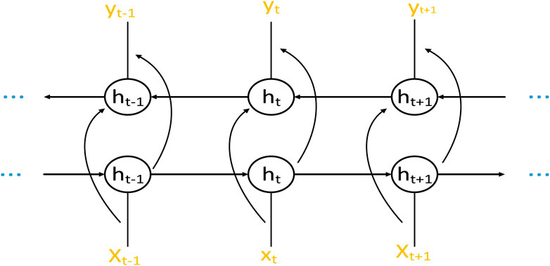
The Bi-LSTM is a neural network with a two-loop structure developed based on LSTM. It consists of a forward LSTM neural network and a reverse LSTM neural network. Data in the forward LSTM neural network flows from the past to the future, utilizing past information, while data in the reverse LSTM flows from the future to the past, utilizing future information.

Figure 8 shows the structure of the neural network, which is the unfolding of the network along the time axis at times t-1, t, and t+1. The network contains a hidden layer, h, which represents the state of the hidden layer. In the figure, h is the state of the hidden layer, x is the input, y is the output, and it includes two hidden layers: forward propagation, and backpropagation. There is no connection between these layers, and the data flows independently in each.

Figure 8

Figure 8. Bi-LSTM structure.

The computation process of the forward LSTM hidden layer state ${\overrightarrow{h}}_t$, and reverse LSTM hidden layer state ${\stackrel{⃖}{h}}_t$ is shown in Equations 12, 13. Both forward and reverse hidden layers can be regarded as single-layer LSTMs, and both can compute their respective hidden layer states h_t from the state at the moment t-1 and the inputs at the moment t. The output of the Bi-LSTM network is the combination of the two parts of the hidden layer states, which constitute the overall hidden state of the network.

${\overrightarrow{h}}_t=LSTM\left(x_t,{\overrightarrow{h}}_{t-1}\right)(12)$

${\stackrel{⃖}{h}}_t=LSTM\left(x_t,{\stackrel{⃖}{h}}_{t-1}\right)(13)$

where ${\overrightarrow{h}}_t$ is the forward LSTM hidden layer state at moment t; ${\stackrel{⃖}{h}}_t$ is the reverse LSTM hidden layer state at moment t; LSTM is the LSTM cell; x_t is the input at moment t.

3.1.6 ED-LSTM neural networks

The ED-LSTM neural network utilizes LSTM neurons to build an encoder-decoder model, where the encoder and decoder parts of the model can each be regarded as an LSTM neural network. The working principle of the ED-LSTM neural network is to convert the model inputs into intermediate vectors of fixed dimensions through the encoding process and then decode the intermediate vectors through the decoding process, predicting the results to be output in combination with the output of the previous moment. The structure of the ED-LSTM neural network is represented in Figure 9:

Figure 9

Figure 9. Framework structure of ED-LSTM.

The encoding process is represented as Equations 14, 15.

$h_t=f\left(h_{t-1},x_t\right)(14)$

$c=q\left(h_1,\cdot \cdot \cdot ,x_t\right)(15)$

where x is the input at moment t; h_t-1 and h_t are the hidden states of the previous moment and this moment; f is a customized nonlinear transformation function; c is an intermediate vector; q is a weighted average function.

The decoding and output process is represented as Equations 16, 17

$s_{t^{\prime }}=f\left(y_{t^{\prime }-1},s_{t^{\prime }-1},c\right)(16)$

$y_{t^{\prime }}=g\left(y_{t^{\prime }-1},s_{t^{\prime }-1},c\right)(17)$

where $y_{t^{\prime }-1}$ and $s_{t^{\prime }-1}$ are the predicted output and implied state at the previous moment; $y_{t^{\prime }}$ and $y_{t^{\prime }}=g\left(y_{t^{\prime }-1},s_{t^{\prime }},c\right)$ are the predicted output and implied state at the current moment; g is a customized nonlinear transformation function.

3.2 Probabilistic prediction of residential load power stochasticity components

3.2.1 GMM principles and parameter optimization

The GMM is a linear combination of multiple single Gaussian probability density functions, and various probability density distributions can be accurately described by adjusting parameters such as weight coefficients, mean, and covariance matrices of the GMM. GMM has extensive applications in the field of photovoltaic and wind power probability prediction. From the previous characterization of residential load power, it can be seen that the stochastic component of residential load power has a small amplitude and fluctuates irregularly around the zero value, so it is theoretically feasible to fit this component using the GMM. Equation 18 shows the GMM composed of multiple Gaussian distribution functions. In addition to the mean and variance, the GMM includes a weight coefficient parameter, which combines multiple single Gaussian functions to improve the model’s ability to fit data that follow a Gaussian distribution.

$P\left(x|\theta \right)={\displaystyle \sum _{w=1}^W}{a}_w\phi \left(x|{\theta }_w\right)(18)$

where the parameter a_w is the weight coefficient of a Gaussian distribution in the GMM, determined according to the algorithm, and satisfies Equation 19, i.e., the sum of the weights is one.

${\displaystyle \sum _{w=1}^W}{a}_w=1,\left(a\ge 0\right)(19)$

The expression for a single Gaussian function in a GMM is shown in Equation 20.

$\phi \left(x|{\theta }_w\right)=\frac{1}{\sqrt{2\pi }{\sigma }_w}{e}^{\left(-\frac{{\left(x-{\mu }_w\right)}^2}{2{{\sigma }_w}^2}\right)}(20)$

where μ_w is the mean of the wth Gaussian distribution member and ${{\sigma }_w}^2$ is the covariance matrix of the wth Gaussian distribution member.

To improve the accuracy of parameter optimization, this paper uses the maximized likelihood function to optimize the three parameters (Xie et al., 2024b). The mathematical expression is shown in Equation 21.

$L\left(x_1,x_2,...;\theta \right)={\displaystyle \prod _{i=1}^m}p\left(x_i,\theta \right)(21)$

The sample data set also contains unobserved hidden variables Z = {z₁, z₂, … }. If the parameters of the mixture model are estimated directly by solving the maximum value of the likelihood estimation function, it will make the parameter-solving process very cumbersome and complicated, making optimization difficult (Yin et al., 2024). Therefore, it is necessary to first find the hidden variables. After identifying the hidden variables, taking the logarithm of the likelihood function yields the following mathematical expression:

$L^{\left(1\right)}\left(x_1,x_2,...;\theta \right)={\displaystyle \sum _{i=1}^m}\log p\left(x_i,\theta \right)={\displaystyle \sum _{i=1}^m}\log {\displaystyle \sum _{z_i}}p\left(x_i,z_i,\theta \right)(22)$

From Equation 22, the likelihood function changes as the parameter set θ changes, and the optimal parameter set θ needs to be determined. The process of solving the maximum likelihood estimation of θ becomes complicated due to the inclusion of the hidden variable Z in the sample dataset, which makes it difficult to optimize the parameters. Therefore, in this paper, the EM algorithm is utilized to estimate the maximum likelihood of the complete data to obtain the optimal parameters.

3.2.2 Randomness component generation methods

To test the prediction performance, it is necessary to combine the prediction results of the deterministic component with those of the stochastic component to obtain the final prediction results. However, the prediction result of the stochastic component of residential load power is a probability density function (PDF), which cannot be directly added to the point prediction result of the deterministic component. Therefore, this paper adopts a method to generate the stochastic component by creating a sample set that conforms to the target distribution. Random samples are then drawn from this set and combined with the prediction result of the deterministic component.

The optimal parameters of the GMM are obtained by the EM algorithm, resulting in the following probability density function (PDF) and cumulative distribution function (CDF), as shown in Equation 23.

$\left\{\begin{array}{l}PDF:f\left(x\right)={\displaystyle \sum _{w=1}^{W_{opt}}}{a}_w\frac{1}{\sqrt{2\pi }{\sigma }_w}{e}^{-{\left(x-{\mu }_w\right)}^2/2{\sigma }_w^2}\\ CDF:F\left(x\right)=\frac{\sqrt{2\pi }}{2}{\displaystyle \sum _{w=1}^{W_{opt}}}{a}_w{\sigma }_w\left[1+\mathit{erf}\left(\frac{x-{\mu }_w}{\sqrt{2}{\sigma }_w}\right)\right]\end{array}\right.(23)$

where a_w, μ_w and σ_w represent the parameters of the wth Gaussian function, W is the total number of Gaussian functions. erf (x) is the Gaussian error function and W_opt is the number of optimal Gaussian functions.

Based on the Newton-Raphson method, a procedure for generating samples of probability distributions is proposed. Set the error threshold η_cdf to 10^–4, divide the parameter $x\in \left[x_{st},x_{en}\right]$ into M segments, and the interval of the mth segment is ${\left[x_{st}+\left(m-1\right)x_{dis},x_{st}+m{x}_{dis}\right]}_m$, where $x_{dis}=\left(x_{en}-x_{st}\right)/M$. Generate a random number r between 0 and 1, find the value of m that meets the condition $F\left(x_{st}+\left(m-1\right)x_{dis}\right)<r<F\left(x_{st}+m{x}_{dis}\right)$, and define it as m_sel. Let $x_1=x_{st}+\left(m_{sel}-1\right)x_{dis}$, and find the value of x when it meets $\left|x_{k+1}-x_k\right|<{\eta }_{cdf}$ according to Equation 24.

$x_{k+1}=x_k-\frac{\frac{\sqrt{2\pi }}{2}{\displaystyle \sum _{i=1}^{W_{opt}}}{a}_w{\sigma }_w\left[1+\mathit{erf}\left(\frac{x_k-{\mu }_w}{\sqrt{2}{\sigma }_w}\right)\right]-r}{{\displaystyle \sum _{w=1}^{W_{opt}}}{a}_w{e}^{-\frac{1}{2}\frac{{\left(x-{\mu }_w\right)}^2}{{\sigma }_w^2}}}(24)$

4 Case studies

4.1 Data processing and evaluation indicators

If the raw data is used as input variables for prediction, it is necessary to normalize the data due to the large range of the data itself, which can affect the efficiency and accuracy of the model’s prediction. The data values were all scaled between 0 and 1 according to Equation 25.

$x^{\prime }=\frac{x-x_{\min }}{x_{\max }-x_{\min }}(25)$

where x and x' are the values of the variables before and after normalization, respectively; x_min and x_max are the minimum and maximum values of the sample variables, respectively.

To test the validity of the model and evaluate the prediction performance, the root mean square error (RMSE) is selected as the evaluation metric in this paper. The formula for the root mean square error is shown in Equation 26.

$RMSE=\sqrt{\frac{1}{n}{\displaystyle \sum _{i=1}^n}{\left(y_i^{\prime }-y_i\right)}^2}(26)$

where n is the number of samples; y_i and y_i^’ are the actual and predicted values of residential load power, respectively.

4.2 Simulation environment and parameters

The prediction of deterministic components of this experiment is done based on the Pycharm development environment. The Keras deep learning framework was selected and ReLU was chosen as the excitation function. The number of iterations is set to 1,000. The optimizer is chosen as Adam optimizer, and for MLP neural networks Adam optimizer and SGD optimizer are chosen for prediction. In this paper, mean square error is used as a loss function. The number of samples for training once is 64.

The prediction of the stochasticity component is done based on the MATLAB platform. The residential load data is modeled using GMM and the parameters are fitted using the EM algorithm, finally, the data is sampled using the stochastic component generation method and the obtained data is added to the deterministic component prediction results to get the final prediction results.

4.3 Analysis of experimental results

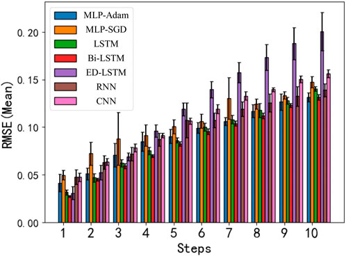
The results of the short-term prediction of the deterministic component of residential load power are shown in Figure 10. In the figure, the horizontal axis represents the number of steps ahead, and the vertical axis represents the normalized RMSE mean. From the figure, it can be seen that the prediction performance of the Bi-LSTM neural network is better than that of other methods, with its RMSE for each step being below 0.14, and the RMSE for the first five steps being below 0.1, which achieves the best prediction performance. Therefore, in this paper, the Bi-LSTM neural network is chosen as the prediction method for the deterministic component of this dataset.

Figure 10

Figure 10. Mean RMSE for ten-step over-forecasting.

The prediction results of Bi-LSTM with ten steps ahead are shown in Figure 11. It can be observed that the prediction performance is relatively good and very close to the actual values, while the prediction error gradually increases with the number of steps ahead, which is consistent with the description in Figure 10.

Figure 11

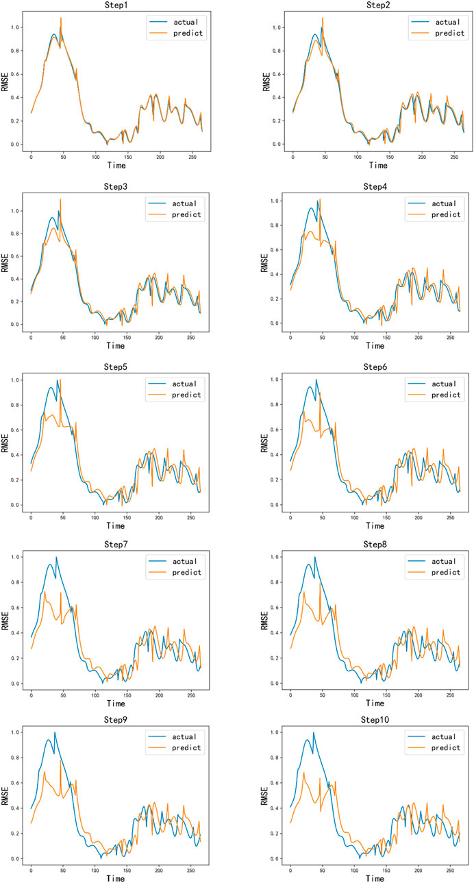
Figure 11. Residential load power deterministic component Bi-LSTM ten-step ahead short-term prediction result.

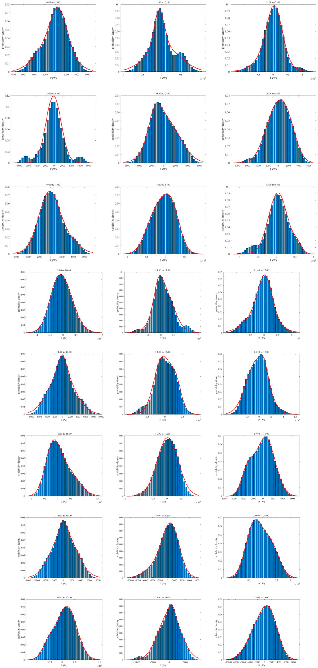
In this paper, a probabilistic forecasting method is used to fit the probability density function of the stochasticity component for each period throughout the day based on the historical data, using a GMM containing two Gaussian members. This is utilized as the probabilistic forecasting result for the stochasticity component. The probabilistic prediction results for the stochastic component of residential load power are shown in Figure 12. From the figure, it can be observed that the probability distribution for most periods is approximately normal and single-peaked. Since the characteristics of the stochastic component are similar to noise, which typically follows a normal distribution, the prediction results are consistent with the expected characteristics of the stochastic component. Additionally, the fitted probability density functions are mostly single-peaked, with a few double-peaked, indicating that it is reasonable to use a GMM consisting of two Gaussian members.

Figure 12

Figure 12. Residential load power stochasticity component PDF.

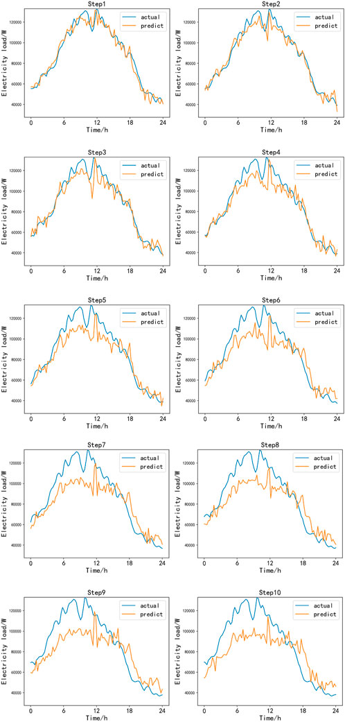
The best prediction method for the short-term prediction of the deterministic component of residential load power is the Bi-LSTM neural network. This method is used to predict the deterministic component, and inverse normalization is performed to obtain the final prediction results for the deterministic component. Random samples are drawn from the probabilistic prediction results of the stochastic component of residential load power for 24 time periods throughout the day, with four samples taken from each period in turn as the simulated prediction value of the stochastic component at each moment of the period. Finally, the two components are added together to form the final prediction results, which are then compared with the actual values.

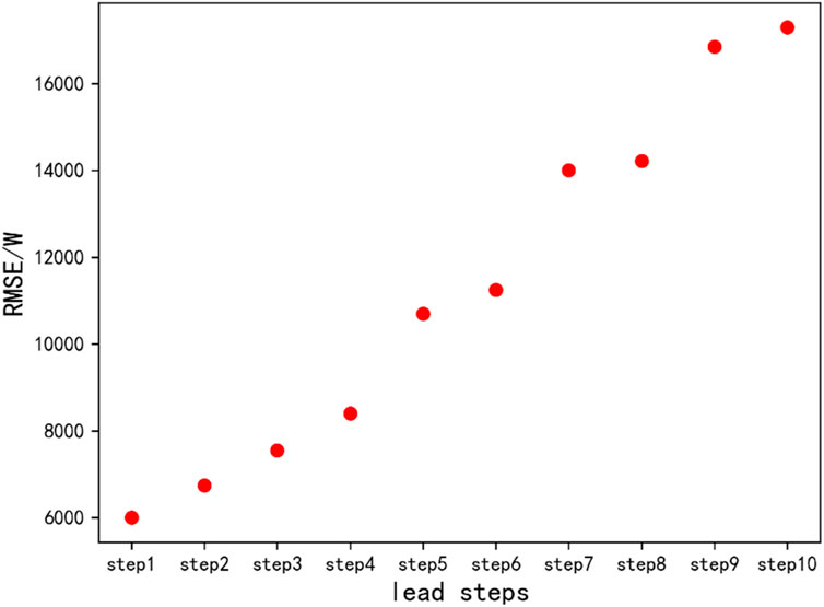
From Figure 13, it can be observed that the overall prediction performance is good. The residential load power data values are distributed between 40 kW and 120 kW, which is about 70 kW at 0:00, then gradually increases and reaches a peak of about 130 kW in the morning hours, and then gradually decreases to about 40 kW. The prediction results of the first few steps are close to the actual values, while the prediction waveforms deviate from the actual values and the prediction errors gradually increase as the number of oversteps increases. The prediction error for each step is shown in Figure 14. The prediction error RMSE for Steps 1 through 4 is around 0.8 kW, while beyond Step 4, the RMSE increases by approximately 1.5 kW on average for each additional step.

Figure 13

Figure 13. Residential load power overrun ten-step prediction results.

Figure 14

Figure 14. Prediction error of ten steps ahead of residential load power.

The Bi-LSTM neural network achieved the best results in predicting residential load power, so this neural network was used to directly predict the raw data. The prediction results were then compared with the results of the prediction model developed in this paper to assess the practicality of the proposed model. The comparison of the over-prediction errors for each step of the point prediction of the raw residential load power data using the Bi-LSTM neural network and the prediction model proposed in this paper is shown in Table 1. Method 1 in the table represents the traditional point prediction method, while method 2 represents the prediction model proposed in this paper. To observe the pattern more clearly, a comparison graph of the two methods is shown in Figure 15.

Table 1

Table 1. Comparative study between traditional point prediction methods and the prediction model developed in this paper.

Figure 15

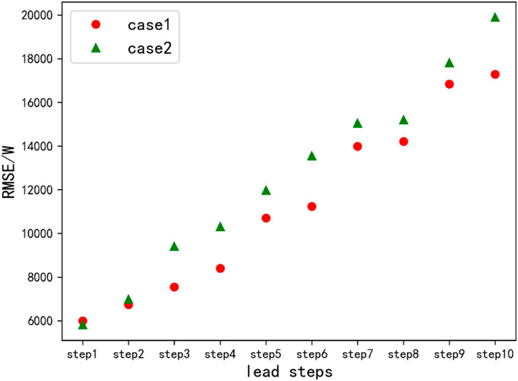
Figure 15. Comparison of prediction errors between traditional point prediction methods and the prediction model developed in this paper.

In Figure 15, case 1 represents the traditional point prediction method, and case 2 represents the model developed in this paper. For residential load power, the prediction model developed in this paper shows a larger error compared to the traditional point prediction model for the first step ahead. However, the performance of the model developed in this paper surpasses that of the direct point prediction method in the subsequent nine steps. It can be observed that the direct point prediction method on the original data has a smaller error when the number of steps ahead is small, while the prediction model developed in this paper has a smaller error when the number of steps ahead is large.

5 Conclusion

This paper highlights the critical role of accurate power prediction in the context of residential load forecasting, addressing the challenges posed by increasing variability and complexity in modern power systems. We conducted a comprehensive analysis using six neural network architectures—MLP, CNN, RNN, LSTM, Bi-LSTM, and ED-LSTM—to predict residential load power, focusing on short-term forecasting accuracy. Our results demonstrated that the Bi-LSTM neural network consistently outperformed the other models, achieving the lowest mean RMSE of 0.086 in ten-step-ahead predictions. This superior performance underscores the effectiveness of Bi-LSTM in capturing the temporal dependencies and nonlinearities inherent in residential load power data, making it the most suitable method for point prediction in this study. Building on the strengths of the Bi-LSTM model, we introduced a novel hybrid prediction framework that integrates neural network-based point prediction with a probabilistic prediction model. This innovative approach not only leverages the time-series forecasting capabilities of neural networks but also incorporates stochastic elements through probabilistic modeling, thereby enhancing the overall accuracy of residential load power predictions. The proposed method was rigorously tested and validated against traditional point prediction models, showing significant improvements in prediction accuracy, particularly in scenarios with higher levels of uncertainty and variability. These results confirm the practicality and effectiveness of our approach, which represents a meaningful advancement in the field of residential load forecasting.

In summary, this study contributes to the literature by demonstrating the superior performance of Bi-LSTM in short-term residential load forecasting and by introducing a hybrid prediction framework that effectively combines deterministic and probabilistic elements. This work not only improves forecasting accuracy but also provides a robust foundation for future research and practical applications in power system management. In this paper, the research object is the prediction of residential load power, while other types of loads such as commercial, office-type loads, and photovoltaic power generation are not studied at present. Since different types of loads have their characteristics, it is important to study the forecasting of other types of loads, which is our next research goal.

Data availability statement

The original contributions presented in the study are included in the article/supplementary material, further inquiries can be directed to the corresponding author.

Author contributions

LZ: Conceptualization, Funding acquisition, Methodology, Project administration, Supervision, Writing–original draft, Writing–review and editing. YZ: Data curation, Formal Analysis, Investigation, Visualization, Writing–review and editing. LL: Data curation, Investigation, Software, Writing–review and editing. XZ: Methodology, Validation, Writing–review and editing.

Funding

The author(s) declare that financial support was received for the research, authorship, and/or publication of this article. This work was supported by East China Branch of State Grid Corporation of China (No. SGHD0000DKJS2310446).

Conflict of interest

Authors LZ, YZ, and LL were employed by East China Branch of State Grid Corporation.

Author XZ was employed by AINERGY LLC.

The authors declare that this study received funding from State Grid Corporation of China. The funder had the following involvement in the study: inspiring the study design, providing basic data collection and practical engineering scenario description.

Publisher’s note

All claims expressed in this article are solely those of the authors and do not necessarily represent those of their affiliated organizations, or those of the publisher, the editors and the reviewers. Any product that may be evaluated in this article, or claim that may be made by its manufacturer, is not guaranteed or endorsed by the publisher.

References

Cao, Z. N., Wang, J. Z., Yin, L., Wei, D. X., and Xiao, Y. Y. (2023). A hybrid electricity load prediction system based on weighted fuzzy time series and multi-objective differential evolution. Appl. Soft Comput. 149, 111007. doi:10.1016/j.asoc.2023.111007

CrossRef Full Text | Google Scholar

Chen, Y. B., Xiao, C., Yang, S., Yang, Y. F., and Wang, W. R. (2024). Research on long term power load grey combination forecasting based on fuzzy support vector machine. Comput. Electr. Eng. 116, 109205. doi:10.1016/j.compeleceng.2024.109205

CrossRef Full Text | Google Scholar

Cui, C., He, M., Di, F. C., Lu, Y., Dai, Y. H., and Lv, F. Y. (2020). “Research on power load forecasting method based on LSTM model,” in Proceedings of 2020 IEEE 5th Information Technology and Mechatronics Engineering Conference, Chongqing, China, 12-14 June 2020, 1657–1660.

CrossRef Full Text | Google Scholar

Gao, F. (2019). “Application of improved grey theory prediction model in medium-term load forecasting of distribution network,” in 2019 Seventh International Conference on Advanced Cloud and Big Data, Suzhou, China, Sept. 21 2019-Sept. 22 2019, 151–155. doi:10.1109/CBD.2019.00036

CrossRef Full Text | Google Scholar

Gao, Y., Sun, K., Qiu, W., Li, Y., Li, M., and Sun, Y. (2024). Data-driven multidimensional analysis of data reliability's impact on power supply reliability. IEEE Trans. Industrial Inf., 1–11. doi:10.1109/TII.2024.3435368

CrossRef Full Text | Google Scholar

Huang, H., Wang, J. X., Xiao, Y. P., Liang, J. B., Guo, J. C., and Ma, Q. (2024). Key technologies and research framework for the power and energy balance analysis in new-type power systems. Electr. Power Constr. 45 (9), 1–12. doi:10.12204/j.issn.1000-7229.2024.09.001

CrossRef Full Text | Google Scholar

Huang, L., Zhang, C., and Yu, P. (2020). Research on power load forecast based on ceemdan optimization algorithm. J. Phys. Ser. 1634, 012142. doi:10.1088/1742-6596/1634/1/012142

CrossRef Full Text | Google Scholar

Jin, X. B., Wang, H. X., Wang, X. Y., Bai, Y. T., Su, T. L., and Kong, J. L. (2020). Deep-learning prediction model with serial two-level decomposition based on bayesian optimization. Complexity 2020, 1–14. doi:10.1155/2020/4346803

CrossRef Full Text | Google Scholar

Li, J. F., Zou, N., and Wu, J. (2023a). “Power supply zonal loads prediction considering matching of contact line characteristics based on deep transfer learning,” in 2023 IEEE IAS Industrial and Commercial Power System Asia, Chongqing, China, 07-09 July 2023, 225–231. doi:10.1109/ICPSASIA58343.2023.10294849

CrossRef Full Text | Google Scholar

Li, M., Tian, H. W., Chen, Q. H., Zhou, M. L., and Li, G. (2024). A hybrid prediction method for short-term load based on temporal convolutional networks and attentional mechanisms. IET Generation Transm. Distribution 18 (5), 885–898. doi:10.1049/gtd2.12798

CrossRef Full Text | Google Scholar

Li, Y. H., Sun, Y. Y., Wang, Q. Y., Sun, K. Q., Li, K. J., and Zhang, Y. (2023b). Probabilistic harmonic forecasting of the distribution system considering time-varying uncertainties of the distributed energy resources and electrical loads. Appl. Energy 329, 120298. doi:10.1016/j.apenergy.2022.120298

CrossRef Full Text | Google Scholar

Liao, W. L., Ge, L. J., Bak-Jensen, B., Pillai, J. R., and Yang, Z. (2022). Scenario prediction for power loads using a pixel convolutional neural network and an optimization strategy. Energy Rep. 8, 6659–6671. doi:10.1016/j.egyr.2022.05.028

CrossRef Full Text | Google Scholar

Lu, Y. L., Teng, Y. L., and Wang, H. (2019). Load prediction in power system with grey theory and its diagnosis of stabilization. Electr. Power Components Syst. 47 (6-7), 619–628. doi:10.1080/15325008.2019.1587648

CrossRef Full Text | Google Scholar

Ning, Y., Zhang, T. Y., and Zhang, T. (2021). The application of improved neural network algorithm based on particle group in short-term load prediction. 2020 ASIA Conf. Geol. Res. Environ. Technol. 632, 042045. doi:10.1088/1755-1315/632/4/042045

CrossRef Full Text | Google Scholar

Sun, K. Q., Qiu, W., Yao, W. X., You, S. T., Yin, H., and Liu, Y. L. (2021). Frequency injection based HVDC attack-defense control via squeeze-excitation double CNN. IEEE Trans. Power Syst. 36 (6), 5305–5316. doi:10.1109/TPWRS.2021.3078770

CrossRef Full Text | Google Scholar

Sun, Q., and Cai, H. F. (2022). Short-term power load prediction based on VMD-SG-LSTM. IEEE Access 10, 102396–102405. doi:10.1109/ACCESS.2022.3206486

CrossRef Full Text | Google Scholar

Wang, K., Wang, C. F., Yao, W. L., Zhang, Z. W., Liu, C., Dong, X. M., et al. (2024a). Embedding P2P transaction into demand response exchange: a cooperative demand response management framework for IES. Appl. Energy 367, 123319. doi:10.1016/j.apenergy.2024.123319

CrossRef Full Text | Google Scholar

Wang, Z. K., Wu, J. Y., Xin, R., Bai, T., Zhao, J. B., Wei, M. L., et al. (2020). “Research on power network load forecasting problem based on machine learning,” in 2019 5th International Conference on Green Materials and Environmental Engineering, Guangzhou, China, December 27-29, 2019, 012055. doi:10.1088/1755-1315/453/1/012055

CrossRef Full Text | Google Scholar

Wang, Z. X., Ku, Y. Y., and Liu, J. (2024b). The power load forecasting model of combined SaDE-ELM and FA-CAWOA-SVM based on CSSA. IEEE Access 12, 41870–41882. doi:10.1109/ACCESS.2024.3377097

CrossRef Full Text | Google Scholar

Wu, D. (2017). Power load prediction based on GM (1,1). Materials Science. Energy Technol. Power Eng. I, 1839. doi:10.1063/1.4982405

CrossRef Full Text | Google Scholar

Xia, Y., Yu, S., Jiang, L., Wang, L. M., Lv, H. H., and Shen, Q. Z. (2023). Application of fuzzy support vector regression machine in power load prediction. J. Intelligent Fuzzy Syst. 45 (5), 8027–8048. doi:10.3233/JIFS-230589

CrossRef Full Text | Google Scholar

Xie, X. M., Ding, Y. H., Sun, Y. Y., Zhang, Z. S., and Fan, J. H. (2024a). A novel time-series probabilistic forecasting method for multi-energy loads. Energy 306, 132456. doi:10.1016/j.energy.2024.132456

CrossRef Full Text | Google Scholar

Xie, X. M., Zhang, J. H., Sun, Y. Y., and Fan, J. H. (2024b). A measurement-based dynamic harmonic model for single-phase diode bridge rectifier-type devices. IEEE Trans. Instrum. Meas. 73, 1–13. doi:10.1109/TIM.2024.3370782

CrossRef Full Text | Google Scholar

Xiong, X., Xu, Z. Y., and Yuan, Y. X. (2022). Grey correlation-oriented random forest and particle swarm optimization algorithm for power load forecasting. J. Appl. Sci. Eng. 25 (1), 19–30. doi:10.6180/jase.202202_25(1).0003

CrossRef Full Text | Google Scholar

Yao, X. T., Fu, X. L., and Zong, C. F. (2022). Short-term load forecasting method based on feature preference strategy and lightGBM-XGboost. IEEE Access 10, 75257–75268. doi:10.1109/ACCESS.2022.3192011

CrossRef Full Text | Google Scholar

Yin, S. L., Sun, Y. Y., Xu, Q. S., Sun, K. Q., Li, Y. H., Ding, L., et al. (2024). Multi-harmonic sources identification and evaluation method based on cloud-edge-end collaboration. Int. J. Electr. Power and Energy Syst. 156, 109681. doi:10.1016/j.ijepes.2023.109681

CrossRef Full Text | Google Scholar

Yudantaka, K., Kim, J. S., and Song, H. (2020). Dual deep learning networks based load forecasting with partial real-time information and its application to system marginal price prediction. Energies 13 (1), 148. doi:10.3390/en13010148

CrossRef Full Text | Google Scholar

Zhang, J. L., Wang, S. Y., Tan, Z. F., and Sun, A. L. (2023). An improved hybrid model for short term power load prediction. Energy 268, 126561. doi:10.1016/j.energy.2022.126561

CrossRef Full Text | Google Scholar

Zhang, Z. W., Wang, C. F., Wu, Q. W., and Dong, X. M. (2024). Optimal dispatch for cross-regional integrated energy system with renewable energy uncertainties: a unified spatial-temporal cooperative framework. Energy 292, 130433. doi:10.1016/j.energy.2024.130433

CrossRef Full Text | Google Scholar

Zou, M., and Tao, H. Q. (2014). Power load prediction based on a hybrid forecast algorithm. Appl. Mech. Mater. 448-453, 2516–2519. doi:10.4028/www.scientific.net/AMM.448-453.2516

CrossRef Full Text | Google Scholar